An Optimal Model Identification For Oscillatory Dynamics With a Stable Limit Cycle

Abstract

We propose a general framework for parameter-free identification of a class of dynamical systems. Here, the propagator is approximated in terms of an arbitrary function of the state, in contrast to a polynomial or Galerkin expansion used in traditional approaches. The proposed formulation relies on variational data assimilation using measurement data combined with assumptions on the smoothness of the propagator. This approach is illustrated using a generalized dynamic model describing oscillatory transients from an unstable fixed point to a stable limit cycle and arising in nonlinear stability analysis as an example. This 3-state model comprises an evolution equation for the dominant oscillation and an algebraic manifold for the low- and high-frequency components in an autonomous descriptor system. The proposed optimal model identification technique employs mode amplitudes of the transient vortex shedding in a cylinder wake flow as example measurements. The reconstruction obtained with our technique features distinct and systematic improvements over the well-known mean-field (Landau) model of the Hopf bifurcation. The computational aspect of the identification method is thoroughly validated showing that good reconstructions can also be obtained in the absence of of accurate initial approximations.

Keywords: hydrodynamic instabilities, reduced-order models, mean-field models, variational data assimilation, adjoint-based optimization,

AMS subject classifications: 93A30, 65K10, 76D25

1 Introduction

In this study we consider the problem of parameter-free identification of a class of dynamical systems. The approach we propose is derived from a general method for the reconstruction of the constitutive relations in systems described by partial differential equations (PDEs) which was initially introduced in [1] and further developed in [2], see also [3]. The idea is that, given an autonomous evolution equation $\frac{d}{dt}\bm{a}=\bm{f}(\bm{a})$ for some quantity ${\mathbf{a}}(t)$ (defined in a finite or infinite dimension with $t\geq 0$ denoting time), one seeks to optimally reconstruct the flux function ${\mathbf{f}}({\mathbf{a}})$, so that the system outputs best match, in a suitably defined sense, with the measurements available. As shown schematically in Figure 1, the originality of this approach is that the function ${\mathbf{f}}({\mathbf{a}})$ is reconstructed directly as a continuous object, rather than employing a truncated polynomial or other Galerkin expansion. In [1, 2, 3] we reviewed the mathematical foundations and some computational aspects of this approach applied to the reconstruction of state-dependent transport coefficients in a class of systems described by PDEs. In the present investigation we adapt this method to the problem of identification of the propagator function $\bm{f}\;:\;{\mathbb{R}}^{N}\rightarrow{\mathbb{R}}^{N}$, $\bm{f}=[f_{1},\ldots,f_{N}]^{T}$, in a finite-dimensional dynamical system $\frac{d}{dt}\bm{a}=\bm{f}(\bm{a})$ with the state vector $\bm{a}(t)=[a_{1}(t),\ldots,a_{N}(t)]^{T}\in{\mathbb{R}}^{N}$. To fix attention, instead of working with an abstract formulation, we will focus on a specific problem concerning a three-dimensional ($N=3$) model characterized by oscillatory dynamics with a stable limit cycle. In many real-life physical problems with infinite-dimensional state spaces and evolution described by PDEs such systems arise as reduced-order models providing low-dimensional approximate description in the neighborhood of fixed points and limit cycles.

         Standard Approach: • Step 1 — select model dimension $N$, • Step 2 — identify structure, e.g., $$\frac{d}{dt}a\approx\sum_{k=0}^{N}c_{k}\,a^{k},\hfill\hskip 42.67912pt(\star)$$ • Step 3 — identify parameters $\{c_{k}\}_{k=0}^{N}$.    Proposed Approach: • Step 1 — select model dimension $N$, • Step 2 — perform parameter-free reconstruction of $f(a)$ using the variational technique described below, • Step 3 — truncate the reconstructed function to a suitable form such as, e.g., ($\star$).

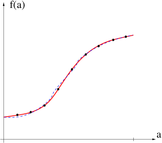
Figure 1: Schematic diagram illustrating the main idea behind (a) the standard approach and (b) the proposed new approach to model identification. In the figures the solid line represents the “true” descriptor function $f(a)$, whereas the dashed lines denote its reconstructions obtained with the two approaches. In Figure (b) the solid symbols represent the grid points used for the discretization of the variational formulation.

In some cases propagator ${\mathbf{f}}$ may be derived from the description of the full plant based on first principles. In general, however, the reduced-order model is inferred from experimental or numerical data. Such reduced models are of paramount importance as test-beds for the development of our understanding of system dynamics. They are also useful as low-cost surrogates guiding optimization and real-time control design for expensive full-scale models. In all cases, typical model identification is generally performed in three steps: (1) selection of the state space ${\mathbb{R}}^{N}$ which is large enough to capture the behaviour of interest and at the same time sufficiently small to allow one to exploit the analytical/numerical advantages of the surrogate plant; (2) structure identification of the propagator $\bm{f}$, e.g., determination of the polynomial degree of its components $f_{i}$, $i=1,\dots,N$; and (3) parameter identification, e.g., inference of the polynomial coefficients from time-resolved trajectories $t\mapsto\bm{a}(t)$. These different steps are illustrated schematically in Figure 1a. The challenge of this approach is to find the right balance between the robustness of the model identification, requiring only a few tunable parameters, and a good accuracy for which a larger number of parameters is typically needed. Identification problems can also be solved using variational techniques and this is the approach we will pursue in the present study, cf. Figure 1b. Similar methods have been developed for a broad range of problems in both the finite and infinite-dimensional setting, including flow control in fluid mechanics [4], data assimilation in meteorology [5, 6] and geophysics [7] to mention just a few application areas. The related problem of state estimation is usually solved using various filtering approaches such as the Kalman filter [8].

We introduce now our model. The oscillatory fluctuation is parameterized by

$$a_{1}+\imath a_{2}=r\>\exp(\imath\theta),$$ (1)

where $\imath$ is the imaginary unit, $r:=\sqrt{a_{1}^{2}+a_{2}^{2}}$ is the amplitude of the fluctuation (“$:=$” means “equal to by definition”) and $\theta:=\arctan(a_{2}/a_{1})$ the corresponding phase, while the base-flow deformation is characterized by a single parameter $a_{3}$. Following the mean-field theory [9], we make the following assumptions about the structure of the system:

Assumption 1

1. In the plane $(a_{1},a_{2})$ the system exhibits an unstable fixed point at the origin and an attracting limit cycle,

2. the state variable $a_{3}$ is “slaved” to $a_{1}$ and $a_{2}$, i.e., $a_{3}=a_{3}(a_{1},a_{2})$, and

3. the dynamics is phase-invariant, i.e., the descriptor system depends only on $r$.

As regards the time $t$, we will assume that $t\in[0,T]$ for some $T>0$. As a general form of a dynamical system consistent with Assumption 1 we will consider

$$\dot{r}{(t)} =g_{1}(r{(t)})\>r{(t)},$$ (2a)

$$\dot{\theta}{(t)} =g_{2}(r{(t)}),$$ (2b)

$$a_{3}{(t)} =g_{3}(r{(t)}),$$ (2c)

or, equivalently

$$\frac{d}{dt}\begin{bmatrix}a_{1}(t)\\ a_{2}(t)\end{bmatrix} =\left(g_{1}(r)\,{\bf I}+g_{2}(r)\,{\bf J}\right)\begin{bmatrix}a_{1}(t)\\ a_{2}(t)\end{bmatrix}=:\begin{bmatrix}f_{1}\\ f_{2}\end{bmatrix},$$ (3a)

$$a_{3}(t) =g_{3}(r(t)),$$ (3b)

where ${\bf I}=\begin{bmatrix}1&0\\ 0&1\end{bmatrix}$ and ${\bf J}=\begin{bmatrix}0&-1\\ 1&0\end{bmatrix}$. Subsequently, we will also use the notation $\bm{\xi}:=[a_{1},\ a_{2}]^{T}$ and ${\mathcal{I}}:=[0,\ r_{max}]$, where $r_{max}:=\sup_{t\in[0,T]}r(t)$. We note that the equations governing $a_{1}$ and $a_{2}$, or equivalently $r$ and $\theta$, do not depend on $a_{3}$. Equations (2c) and (3b) describe the dependency of a slow variable on the fluctuation amplitude, and the usefulness of these algebraic equations will become clear in the context of the mean-field models discussed in Section 2.3. In (2) and (3) the functions $g_{i}\;:\;{\mathcal{I}}\rightarrow{\mathbb{R}}$, $i=1,2,3$, are assumed sufficiently regular to make the systems well posed (the question of the regularity of functions $g_{i}$, $i=1,2,3$, will play an important role in our approach and will be addressed in detail further below). Without loss of generality, we will also assume that $\dot{\theta}\geq 0$. System (3a), or (2a)–(2b), is complemented with the initial condition, respectively, $\bm{\xi}(0)=\bm{\xi}^{0}:=[a_{1}^{0},\ a_{2}^{0}]^{T}$ and $r(0)=\|\bm{\xi}^{0}\|$, $\theta(0)=\arctan(a_{2}^{0}/a_{1}^{0})$. Dynamical systems of the type (2) or (3) arise commonly as a result of various rigorous and empirical model-reduction strategies in diverse application areas such as fluid mechanics [10], thermodynamics [11] and phase transitions [12]. The main contribution of this work is development of a computational technique allowing one to reconstruct functions $g_{1}$, $g_{2}$ and $g_{3}$ in (2) in a very general form based on some measurements. The key idea is to formulate a least-squares minimization problem in which one of the functions $g_{i}$, $i=1,2,3$, is the control variable. Then, a variational gradient-based approach can be employed to find the optimal solution in a suitable function space.

In the present investigation, we will consider system (2) as a reduced-order model of hydrodynamic instabilities in open shear flows obtained using a suitable Galerkin projection — to fix attention without losing generality. Although this problem is very well-studied, our method provides a systematic refinement of the state-of-the-art mean-field model, which is the second main contribution of this study. Details of this problem are introduced in the next Section. In the following Section we develop our model identification approach, whereas in Section 4 we present a number of computational results concerning identification of the model for the system considered in Section 2. Then, in Section 5, we analyze the computational performance of our method and discuss the improvements it offers over the predictions of some standard models applied to the problem in question. Summary and conclusions are deferred to Section 6, whereas in Appendices A, B and C we collect some technical results.

2 Example Problem — Model Identification For a Vortex Shedding Instability

In this Section we define a model identification problem associated with the transient two-dimensional (2D) cylinder wake which is a well-studied hydrodynamic instability [13, 14, 15]. This flow is a representative example of phenomena characterized by the Hopf bifurcation with an unstable fixed point and a stable limit cycle. Additional examples in this category include the Rossiter modes of the flow over a cavity [16] and other shear flows [17]. First, in Section 2.1, we describe the initial-boundary value problem for the infinite-dimensional Navier-Stokes equation which is a system of coupled PDEs representing the conservation of mass and momentum in the motion of viscous incompressible fluid. Then, in Section 2.2, a low-dimensional Galerkin expansion is recalled which reduces the kinematic description down to three modes whose amplitudes serve as the state variables $a_{1}$, $a_{2}$ and $a_{3}$. It will be demonstrated that the system governing these variables satisfies in fact Assumptions 1 and is in the form (3). Special forms of this system arising as models in numerous applications are discussed in Section 2.3, whereas in Section 2.4 we describe the measurements used as the basis for the reconstructions.

2.1 Cylinder Wake Flow

The 2D flow around a circular cylinder is described here in the Cartesian coordinate system $\bm{x}:=(x,y)$. The origin $\bm{0}$ coincides with the center of the cylinder, the $x$-coordinate points in streamwise direction, while $y$ represents the transverse coordinate. The velocity field $\bm{u}:=(u,v)$ has components $u$ and $v$ aligned with the $x$-axis and $y$-axis, respectively, whereas $p$ represents the pressure field. The oncoming flow velocity is denoted by $U$ and the cylinder diameter by $D$. The Newtonian fluid is characterized by uniform density $\rho$ and kinematic viscosity $\nu$. The flow properties depend on the Reynolds number $Re:=U\>D/\nu$. Here, we consider the case of $Re=100$ which is far above the critical Reynolds number of $47$ characterizing the onset of vortex shedding (i.e., the Hopf bifurcation) [13, 18], and far below the transitional Reynolds number of 187 which marks the onset of three-dimensional instabilities [19].

In the following, all quantities are assumed to be non-dimensionalized with $U$, $D$ and $\rho$. The flow is considered in a rectangular domain surrounding the cylinder

$$\Omega:=\{(x,y)\>\colon\>x^{2}+y^{2}\geq 1/4\>\wedge\>-5\leq x\leq 15\>\wedge\>|y|\leq 5\}$$ (4)

and its evolution is described by the incompressible Navier-Stokes equation

$$\nabla\cdot\bm{u} =0 \textrm{in}\ \Omega,$$ (5a)

$$\partial_{t}\bm{u}+\bm{u}\cdot\nabla\bm{u} =\frac{1}{Re}\triangle\bm{u}-\nabla p \textrm{in}\ \Omega.$$ (5b)

The boundary conditions for the velocity comprise the no-slip condition at the cylinder, the free-stream condition at the inlet boundary, the free-slip condition at the lateral boundaries and the no-stress condition at the downstream outflow boundary. The initial condition for the velocity at $t=0$ is the unstable fixed point $\bm{u}_{s}$ of Navier-Stokes equation (5) perturbed by the real part of the corresponding most unstable stability eigenmode $\bm{u}_{1}^{\star}(\bm{x})$

$$\bm{u}(\bm{x},0)=\bm{u}_{s}(\bm{x})+0.02\>\bm{u}_{1}^{\star}(\bm{x}).$$ (6)

The field $\bm{u}_{1}^{\star}(\bm{x})$ is normalized to have unit $L_{2}(\Omega)$ norm.

The initial-boundary-value problem is numerically integrated with a finite-element method based on an unstructured grid and details are provided in [20]. Figure 2 depicts three flow snapshots corresponding to the initial condition, an intermediate transient state and the flow approaching the limit cycle.

(a)

(b)

(c)

Figure 2: Flow snapshots at (a) $t=0$ (initial condition), (b) $t=24.8$ (intermediate transient state), and (c) $t=99.6$ (periodic solution at the limit cycle). The domain shown represents the computational domain $\Omega$ which also coincides with the region where the Galerkin expansion is defined. The flow patterns are visualized using streamlines (which are defined as the level sets of the streamfunction $\psi\;:\;\Omega\rightarrow{\mathbb{R}}$ related to the velocity components via $u={\partial\psi\over\partial y}$ and $v=-{\partial\psi\over\partial x}$). The cylinder is indicated by the black circle.

2.2 Galerkin Expansion

Below we review approximate modelling approaches typically employed to obtain low-dimensional descriptions of the dynamics described by (5), cf. [21]. The quantities corresponding to the limit cycle will be denoted with the superscript ’$\circ$’ and in the present problem in which the limit cycle is stable we will therefore have $r^{\circ}=r_{max}$. The transient wake is usually characterized by the superposition of a time-varying symmetric base flow $\bm{u}^{B}$ with the length of the recirculating region decreasing with time as the vortex shedding develops and an antisymmetric oscillating field $\bm{u}^{\prime}$ representing the vortex shedding. The change of the base flow is accurately captured by a single “shift mode” $\bm{u}_{\Delta}$ [22], while the oscillation field can be approximated by the first two Proper Orthogonal Decomposition (POD) modes $\bm{u}_{i}$, $i=1,2$, computed at the limit cycle [23, 20]. Hereafter, the subscript ’$\Delta$’ will denote various quantities related to the shift mode $\bm{u}_{\Delta}$. Some information about the construction of orthogonal bases using the POD approach is presented in Appendix A. The resulting truncated Galerkin expansion thus takes the form

$$\bm{u}(\bm{x},t) \approx\bm{u}^{B}(\bm{x},t)+\bm{u}^{\prime}(\bm{x},t),$$ (7a)

$$\bm{u}^{B}(\bm{x},t) =\bm{u}_{s}(\bm{x})+a_{\Delta}(t)\>\bm{u}_{\Delta}(\bm{x}),$$ (7b)

$$\bm{u}^{\prime}(\bm{x},t) =a_{1}(t)\>\bm{u}_{1}(\bm{x})+a_{2}(t)\>\bm{u}_{2}(\bm{x}).$$ (7c)

One typically ignores deformations of the oscillatory modes during the transient. These deformations do not significantly alter the model predictions and do not have any effect on the proposed model identification approach. On the other hand, inclusion of this effect in our model would significantly complicate the study and is outside the scope of this investigation. Identifying $a_{3}=a_{\Delta}$ and assuming phase-invariant behavior, we note that the evolution of the Galerkin expansion coefficients is governed by a system in the form (3), provided that $g_{1}(0)>0$, corresponding to an unstable fixed point at the origin, and $g_{1}(r^{\circ})=0$ and $dg_{1}/dr|_{r=r^{\circ}}<0$, corresponding to a locally attracting limit cycle at $r=r^{\circ}>0$, cf. Assumption 1(a). Moreover, from the assumptions made in Section 1, it follows that $\forall_{r\geq 0}\ g_{2}(r)>0$. Introducing a number of further simplifications one arrives at two well-known reduced models, the Mean-Field Model and the Landau Model. Since they provide a point of reference for our test problems, we describe them briefly below.

2.3 Mean-Field Model

The mean-field model of oscillatory flow instabilities [9] explicates the mechanism of amplitude saturation in the mean-field deformation. This deformation is quantified by the amplitude $a_{\Delta}$ of the shift mode, cf. (7b), which is slaved to the fluctuation level $r$. For the soft (supercritical) Hopf bifurcation, the resulting evolution equations read

$$\dot{r}{(t)} = \left[\sigma_{1}-\beta_{\Delta}\>a_{\Delta}({t})\right]\>r{(t)},$$ (8a)

$$\dot{\theta}{(t)} = \omega_{1}+\gamma_{\Delta}a_{\Delta}({t}),$$ (8b)

$$a_{\Delta}({t}) = \alpha_{\Delta}\>r^{2}{(t)}.$$ (8c)

The ordinary differential equations (8a) and (8b) correspond to the Navier-Stokes equation linearized around the time-varying base flow with $a_{\Delta}$ as the order parameter. The third algebraic equation (8c) represents the Reynolds equation linking the mean flow to the Reynolds stress generated by the fluctuations described by the first equation.

Evidently, equations (8) are a particular case of (3) with $g_{1}(r)=\sigma_{1}-\beta_{\Delta}\>{a_{\Delta}\>r^{2}}$, $g_{2}(r)=\omega_{1}+\gamma_{\Delta}\>{a_{\Delta}\>r^{2}}$ and $g_{3}(r)=\alpha_{\Delta}\>r^{2}$. The parameters $\sigma_{1}$, $\omega_{1}$, $\beta_{\Delta}$, $\gamma_{\Delta}$, $\alpha_{\Delta}$ of (8) may be derived from the Galerkin approximation described in Section 2.2, or identified from the solutions of the Navier-Stokes equation via suitable fitting. The periodic solution of (8) is given by

$$r^{\circ} = \sqrt{\frac{\sigma_{1}}{\alpha_{\Delta}\>\beta_{\Delta}}},$$ (9a)

$$\omega^{\circ}-\omega_{1} = \gamma_{\Delta}\sqrt{\frac{\sigma_{1}}{\beta_{\Delta}}},$$ (9b)

$$a_{\Delta}^{\circ} = \sigma_{1}/\beta_{\Delta}.$$ (9c)

At the limit cycle the mean flow is predicted to have a vanishing growth rate $g_{1}$. This marginal stability property of mean flows has been conjectured by Malkus [24] and is corroborated by the global stability analysis of the Navier-Stokes equation [25]. Derivation details and a further discussion of the properties of the mean-field model can be found in [20].

The Landau equation for the supercritical Hopf bifurcation is a corollary to the mean-field model and constitutes a prototype evolution equation for self-amplified, amplitude-limited oscillations. It is obtained by substituting (8c) in (8a)–(8b):

$$\dot{r} = \sigma_{1}\>r-\beta\>r^{3},$$ (10a)

$$\dot{\theta} = \omega_{1}+\gamma\>r^{2}.$$ (10b)

Here, we require $\sigma_{1},\beta,\omega_{1}>0$ to ensure a stable limit cycle with a positive angular velocity in the $(a_{1},a_{2})$ plane, cf. Assumption 1(a), whereas $\gamma$ may vanish, be positive or negative. Evidently, equations (10) correspond to (8a)–(8b) with $\beta=\alpha_{\Delta}\beta_{\Delta}$ and $\gamma=\alpha_{\Delta}\gamma_{\Delta}$. Therefore, the Landau equation (10) is also easily recognized as a particular case of (2a)–(2b) and (3a), while the mean-field equation (8c) is an example of (2c) and (3b). The dependency of the growth rate and frequency on the shift mode amplitude $a_{\Delta}$ in (8a)–(8b) may in principle be recovered from (2a)–(2b) by inverting (2c) to give $r=r(a_{\Delta})$ and substituting $r(a_{\Delta})$ into (2a)–(2b). This inversion assumes a monotonous dependence of $a_{\Delta}$ on $r$ which is observed in actual wake data. For completeness, we note that the least-order Galerkin model introduced in [20] includes a fast-dynamics equation for $a_{\Delta}$. This dynamic equation is well represented by an inertial manifold $a_{\Delta}=a_{\Delta}(r)$ of the form (2c) or (3b) which ignores short transients.

The Landau equation (10) may also be derived from the first principles, e.g., using a center-manifold reduction method, see, e.g., [26, 27, 28]. The parameters may be identified from solutions of the Navier-Stokes equation with $\sigma_{1}$ and $\omega_{1}$ obtained as the real and imaginary part of the most unstable eigenvalue associated with the Hopf bifurcation, whereas the nonlinearity parameters $\beta$ and $\gamma$ can be inferred from the post-transient amplitude and frequency, $r^{\circ}$ and $\omega^{\circ}$, respectively. In Section 4 we will demonstrate using our proposed approach how the structure of Landau model (10) could be modified to better reproduce the actual behavior.

2.4 Measurements

The state in our approximate model (2) is characterized by three time-dependent mode amplitudes: $a_{1}$, $a_{2}$ and $a_{3}$ and as “measurements” we will consider the functions ${\tilde{a}}_{1}(t)$, ${\tilde{a}}_{2}(t)$ and ${\tilde{a}}_{\Delta}(t)$ which are obtained for $t\in[0,T]$ by solving initial-boundary-value problem (5)-(6) followed by projection, in terms of the inner product defining the POD analysis (cf. Appendix A), of the resulting time-dependent velocity field $\bm{u}(t,\cdot)$ on the modes $\bm{u}_{1}$, $\bm{u}_{2}$ and $\bm{u}_{\Delta}$. The same procedure applies when the velocity field comes from time- and space-resolved measurements. In either case, determination of the shift mode $\bm{u}_{\Delta}$ requires access to the unstable equilibrium $\bm{u}_{s}$, cf. (7b), which typically needs to be obtained numerically. The mean-field model may also be constructed directly from experimental measurements. Let $s(t)$ be, for instance, a pressure or hot-wire signal with a dominant harmonic component corresponding to the vortex shedding. Let $\langle s\rangle(t)$ be the short-time mean value, e.g., a one-period average, and $s^{\prime}(t):=s(t)-\langle s\rangle(t)$ be the fluctuation. Next, let $a_{1}$ and $a_{2}$ be the local cosine and sine component of the fluctuation. These variables may be obtained from a Hilbert transform or, more robustly, from a Morlet transform of the data. Finally, we identify $a_{\Delta}=\langle s\rangle+\hbox{const}$, where the tunable constant shall ensure the correct fixed-point behavior, i.e., $a_{\Delta}=0$ when $r=0$. Then, $a_{1}$, $a_{2}$ and $a_{\Delta}$ may be approximated by the mean-field model. In this case, it is not required that the fixed point be actually reached for the identification of the model. We only need a transient with a range of $r$ values over which the functions $g_{i}$ are identified. In the next Section we introduce a computational approach allowing one to optimally identify the functions $g_{1}(r)$, $g_{2}(r)$ and $g_{3}(r)$ in a suitable class, so that the predictions of system (2) best match in the least-squares sense the data ${\tilde{a}}_{1}$, ${\tilde{a}}_{2}$ and ${\tilde{a}}_{\Delta}$. We note that, alternatively, a system of evolution equations for $a_{1}$, $a_{2}$ and $a_{3}$ may be obtained by substituting ansatz (7a) into momentum equation (5b), and some comparisons between such an approach and the results obtained using the model identification method developed here will be drawn in Section 5.3.

3 Computational Approach

The task of identifying the functions $g_{i}$, $i=1,2,3$, such that the output of system (2) matches certain “measurements” is an example of an inverse problem [7]. What makes this problem somewhat different from typical inverse problems is that the functions sought have the form of “constitutive relations”, in the sense that they depend on the state variables (i.e., the dependent variables in the problem), rather than the independent variables. More specifically, in the problem considered here $g_{i}$, $i=1,2,3$, depend on $r=\sqrt{a_{1}^{2}+a_{2}^{2}}$ as opposed to $t$. Non-parametric formulations of such inverse problems have received some attention in the context of systems described by PDEs [1, 2, 3, 29], but we are not aware of similar approaches applied to the state-space description of dynamical systems.

3.1 Formulation of Optimization Problem

We will look for functions $g_{i}$, $i=1,2,3$, as elements of the Sobolev space $H^{1}({\mathcal{I}})$ of continuous functions with square-integrable gradients on ${\mathcal{I}}$ which is the “identifiability” region defined in Section 1, i.e., the interval spanned by the state variable $r(t)$ during the system evolution, see also [1]. Some additional remarks concerning the regularity of functions $g_{1}$ and $g_{2}$ are presented in Appendix B. In the reconstruction problems considered in this study, the boundary behavior of the reconstructed functions will have to be restricted in different ways. This reflects the fact that system (2) with the reconstructed functions $g_{i}$, $i=1,2,3$, should exhibit the behavior dictated by Assumption 1(a) in specific regions of the phase space, namely, at the equilibrium $r=0$ and at the limit cycle $r=r^{\circ}$. There is some flexibility as regards possible choices and the boundary conditions we adopt will reproduce the behavior described by the mean-field model introduced in Section 2.3. More specifically,

• at the origin $r=0$

  • the Jacobian of the right-hand side (RHS) in equation (2a) should be given by $g_{1}(0)$ which is a priori unknown and is to be determined as a part of the solution of the reconstruction problem; on the other hand, the Jacobian of the RHS in equation (2b) should vanish; this is achieved when the derivatives of both functions $g_{1}$ and $g_{2}$ are set to zero at the origin, i.e.,

    $$\frac{d}{dr}g_{i}(r)\big{|}_{r=0}=0,\qquad i=1,2,$$ (11)

• at the limit cycle $r=r^{\circ}$

  • the RHS of (2a) should vanish resulting in the vanishing of $g_{1}$, i.e.,

    $$g_{1}(r^{\circ})=0,$$ (12)

  • in regard to equation (2b), we will prescribe a given slope $G>0$ of the RHS, i.e.,

    $$\frac{d}{dr}g_{2}(r)\big{|}_{r=r^{\circ}}=G.$$ (13)

We note that, while the boundary behavior described by (11)–(13) at the equilibrium and the limit cycle is the same as in the mean-field model (cf. Section 2.3), the behavior of the constitutive relations $g_{1}$ and $g_{2}$ for intermediate values of the state magnitude $0<r<r^{\circ}$ can be arbitrary and will be determined using our optimal reconstruction procedure. No restrictions are placed on the boundary behavior of function $g_{3}$, cf. (2c).

A convenient way to solve inverse problems is to formulate them as suitable optimization problems [30]. For each of the functions $g_{i}$, $i=1,2,3$, we thus define the corresponding cost functional ${\mathcal{J}}_{i}(g_{i})\;:\;H^{1}({\mathcal{I}})\rightarrow{\mathbb{R}}$ as

$${\mathcal{J}}_{1}(g_{1}) :=\frac{1}{2}\int_{0}^{T}\left[r(t)-{\tilde{r}}(t)\right]^{2}\,dt,$$ (14a)

$${\mathcal{J}}_{2}(g_{2}) :=\frac{1}{2}\int_{0}^{T}\left[e^{\imath\theta(t)}-e^{\imath\tilde{\theta}(t)}\right]^{2}\,dt,$$ (14b)

$${\mathcal{J}}_{3}(g_{3}) :=\frac{1}{2}\int_{0}^{T}\left[g_{3}(r(t))-{\tilde{a}}_{\Delta}(t)\right]^{2}\,dt,$$ (14c)

where ${\tilde{r}}(t):=\sqrt{{\tilde{a}}_{1}(t)^{2}+{\tilde{a}}_{2}(t)^{2}}$, $\tilde{\theta}(t):=\arctan({\tilde{a}}_{2}(t)/{\tilde{a}}_{1}(t))$ and ${\tilde{a}}_{\Delta}(t)$ are the “measurements” obtained as described in Section 2.4. The length $T$ of the assimilation window will be chosen sufficiently long to allow the transient trajectory to settle on the limit cycle. In (14a) and (14b) the functions $r(t)$ and $\theta(t)$ are related to $g_{1}$ and $g_{2}$ via system (2). The optimal reconstructions $\hat{g}_{1}$, $\hat{g}_{2}$, and $\hat{g}_{3}$ are defined as solutions of the following problems

$$(P1)\qquad \hat{g}_{1} :=\operatorname{argmin}_{g_{1}\in H^{1}({\mathcal{I}}),\ \frac{d}{dr}g_{1}(r)|_{r=0}=0,\ g_{1}(r^{\circ})=0}\ {\mathcal{J}}_{1}(g_{1}),$$ (15a)

$$(P2) \hat{g}_{2} :=\operatorname{argmin}_{g_{2}\in H^{1}({\mathcal{I}}),\ \frac{d}{dr}g_{2}(r)|_{r=0}=0,\ \frac{d}{dr}g_{2}(r)|_{r=r^{\circ}}=G}\ {\mathcal{J}}_{2}(g_{2}),$$ (15b)

$$(P3) \hat{g}_{3} :=\operatorname{argmin}_{g_{3}\in H^{1}({\mathcal{I}})}\ {\mathcal{J}}_{3}(g_{3}).$$ (15c)

Below we describe in detail a gradient-based approach to solution of Problem $(P1)$. Problem $(P2)$ has a similar structure and the solution method is essentially the same with some modifications described hereafter. In Problems $P1$ and $P2$ it is assumed that the functions, respectively, $g_{2}$ and $g_{1}$ are fixed. Problem $(P3)$ has a different structure warranting a separate solution approach which will be described further below.

3.2 Gradient-Based Approach to Solution of Problems $(P1)$ and $(P2)$

The minimizer $\hat{g}_{1}$ is characterized by the first-order optimality condition [31] requiring the vanishing of the Gâteaux differential
${\mathcal{J}}_{1}^{\prime}(g_{1};g^{\prime}_{1}):=\lim_{\epsilon\rightarrow 0}\epsilon^{-1}\left[{\mathcal{J}}_{1}(g_{1}+\epsilon g^{\prime}_{1})-{\mathcal{J}}_{1}(g_{1})\right]$, i.e.,

$$\forall_{g^{\prime}_{1}\in H^{1}({\mathcal{I}}),{\ \frac{d}{dr}g^{\prime}_{1}(r)|_{r=0}=0,\ g^{\prime}_{1}(r^{\circ})=0}}\qquad{\mathcal{J}}_{1}^{\prime}(\hat{g}_{1};g^{\prime}_{1})=0,$$ (16)

where $g^{\prime}_{1}$ is an arbitrary perturbation direction. The (local) minimizer can be computed with the following iterative procedure

$$\left\{\begin{aligned} &g_{1}^{(n+1)}&&=g_{1}^{(n)}-\tau^{(n)}\nabla{\mathcal{J}}_{1}(g_{1}^{(n)}),\qquad n=1,\dots,\\ &g_{1}^{(1)}&&=g_{1}^{0},\end{aligned}\right.$$ (17)

where $g_{1}^{0}$ represents the initial guess, $n$ denotes the iteration count and $\nabla{\mathcal{J}}_{1}\;:\;{\mathcal{I}}\rightarrow{\mathbb{R}}$ is the gradient of cost functional ${\mathcal{J}}_{1}$. The length $\tau^{(n)}$ of the step is determined by solving the following line minimization problem

$$\tau^{(n)}=\operatorname{argmin}_{\tau>0}{\mathcal{J}}_{1}\left(g_{1}^{(n)}-\tau\nabla{\mathcal{J}}_{1}(g_{1}^{(n)})\right)$$ (18)

which can be done efficiently using standard techniques such as Brent’s method [32]. For the sake of clarity, formulation (17) represents the steepest-descent method, however, in practice one typically uses more advanced minimization techniques, such as the conjugate gradient method, or one of the quasi-Newton techniques [33]. Evidently, the key element of minimization algorithm (17) is the computation of the cost functional gradient $\nabla{\mathcal{J}}_{1}$. It ought to be emphasized that, while the governing system (3) is finite-dimensional, the gradient $\nabla{\mathcal{J}}_{1}$ is a function of the state magnitude $r$ and as such represents a continuous (infinite-dimensional) sensitivity of cost functional ${\mathcal{J}}_{1}(g_{1})$ to the perturbations $g^{\prime}_{1}=g^{\prime}_{1}(r)$. The fact that the control variable $g_{1}$, and hence also the gradient $\nabla{\mathcal{J}}_{1}$, are functions of the state variable, rather than the independent variable (Figure 3a), will result in cost functional gradients with structure rather different than encountered in typical optimization problems for differential equations (see [2] for some related questions arising in PDE optimization problems).

  

\psfrag{C}[0.8]{${\mathcal{C}}$}\includegraphics[width=243.91124pt]{vars1_02.eps}

\psfrag{xi}[0.8]{$\bm{\xi}(t),\,\bm{\xi}^{*}(t)$}\psfrag{DJ}[0.8]{$\nabla{\mathcal{J}}_{i}(r)$}\psfrag{r}[0.8]{$r$}\psfrag{C}[0.8]{${\mathcal{C}}$}\includegraphics[width=195.126pt]{vars2_02.eps}

Figure 3: (a) Schematic indicating the dependence of the “constitutive relation” on the state magnitude $r$ with the plane $(a_{1},a_{2})$ representing the phase space. Thick red dashed-dotted line: function $g_{i}$, $i=1,2,3$. Thick blue solid line: sample trajectory $[\xi_{1}(t),\ \xi_{2}(t)]^{T}$, $t\in[0,T]$, of system (3a). Black circle: state at time $t_{0}$. (b) Schematic illustrating the relation between the integration variables $dt$ and $dr$, cf. (24). Blue solid line: system trajectory ${\mathcal{C}}$. The state $\bm{\xi}(t)$ (marked with a black point on the trajectory) together with the corresponding adjoint state $\bm{\xi}^{*}(t)$ carry information necessary to evaluate cost functional gradient $\nabla{\mathcal{J}}_{i}(r)$, where $r=\|\bm{\xi}(t)\|$, cf. (26).

In order to identify an expression for the gradient $\nabla{\mathcal{J}}_{1}$, we proceed by computing the Gâteaux differential of the cost functional

$${\mathcal{J}}_{1}(g_{1};g^{\prime}_{1})=\int_{0}^{T}\left[r-{\tilde{r}}\right]r^{\prime}(g_{1};g^{\prime}_{1})\,dt=\int_{0}^{T}\frac{r-{\tilde{r}}}{r}\bm{\xi}^{T}\bm{\xi}^{\prime}\,dt=\Big{\langle}\nabla{\mathcal{J}}_{1}(g_{1}),g^{\prime}_{1}\Big{\rangle}_{{\mathcal{X}}({\mathcal{I}})},$$ (19)

where we used the identity $r^{\prime}=\bm{\xi}^{T}\bm{\xi}^{\prime}/r$ and the last equality is a consequence of the Riesz representation theorem [34] with $\langle\cdot,\cdot\rangle_{{\mathcal{X}}({\mathcal{I}})}$ denoting an inner product in the Hilbert space ${\mathcal{X}}({\mathcal{I}})$ (to be specified later) of functions defined on ${\mathcal{I}}$. The perturbation variable $\bm{\xi}^{\prime}$ is a solution of the following perturbation problem (see Appendix C for a derivation)

$$\dot{\bm{\xi}}^{\prime}(t) =\left[g_{1}(r(t)){\bf I}+{\bf I}\,\bm{\xi}(t)\,(\bm{\nabla}g_{1}(r(t)))^{T}\right.$$

$$\hskip 28.45274pt\left.+g_{2}(r(t)){\bf J}+{\bf J}\,\bm{\xi}(t)\,(\bm{\nabla}g_{2}(r(t)))^{T}\right]\bm{\xi}^{\prime}(t)+{\bf I}\,\bm{\xi}(t)\,g^{\prime}_{1}$$

$$=:{\bf A}(\bm{\xi}(t))\,\bm{\xi}^{\prime}+{\bf I}\,\bm{\xi}(t)\,g^{\prime}_{1},$$ (20a)

$$\bm{\xi}^{\prime}(0) =0,$$ (20b)

where $\bm{\nabla}g_{i}=\left[{\partial g_{i}\over\partial a_{1}},\ {\partial g_{i}\over\partial a_{2}}\right]^{T}$, $i=1,2$. We note that Gâteaux differential (19) is not yet in the form consistent with the Riesz representation, since the perturbation $g^{\prime}_{1}$ does not appear in it as a factor, but is hidden on the RHS in perturbation equation (20a). A standard technique to convert Gâteaux differential (19) to the Riesz form is based on the adjoint variable $\bm{\xi}^{*}\;:\;[0,T]\rightarrow{\mathbb{R}}^{2}$. Taking the inner product (in ${\mathbb{R}}^{2}$) of $\bm{\xi}^{*}(t)$ with equation (20a), integrating over $[0,T]$ and then integrating by parts we obtain

$$\begin{split}0=&\int_{0}^{T}\,\left(\bm{\xi}^{*}\right)^{T}\Big{\{}\dot{\bm{\xi}}^{\prime}-\left[g_{1}(r){\bf I}+{\bf I}\,\bm{\xi}\,(\bm{\nabla}g_{1}(r))^{T}+g_{2}(r){\bf J}+{\bf J}\,\bm{\xi}\,(\bm{\nabla}g_{2}(r))^{T}\right]\bm{\xi}^{\prime}-\bm{\xi}\,g^{\prime}_{1}\Big{\}}\,dt\\ =&\int_{0}^{T}\,\left(\bm{\xi}^{\prime}\right)^{T}\Big{\{}-\dot{\bm{\xi}}^{*}-\left[g_{1}(r){\bf I}+{\bf I}\,\bm{\xi}\,(\bm{\nabla}g_{1}(r))^{T}+g_{2}(r){\bf J}+{\bf J}\,\bm{\xi}\,(\bm{\nabla}g_{2}(r))^{T}\right]^{T}\bm{\xi}^{*}\Big{\}}\,dt\\ &+\Big{[}(\bm{\xi}^{*})^{T}\bm{\xi}^{\prime}\Big{]}_{t=0}^{t=T}-\int_{0}^{T}\,\left(\bm{\xi}^{*}\right)^{T}\,{\bf I}\,\bm{\xi}(t)\,g^{\prime}_{1}\,dt.\end{split}$$ (21)

Defining the adjoint system as

$$-\dot{\bm{\xi}}^{*}(t) =\left[{\bf A}(\bm{\xi}(t))\right]^{T}\bm{\xi}^{*}(t)+\frac{r-{\tilde{r}}}{r}\bm{\xi},$$ (22a)

$$\bm{\xi}^{*}(T) =0,$$ (22b)

we reduce relation (21) to

$${\mathcal{J}}^{\prime}_{1}(g_{1};g^{\prime}_{1})=\int_{0}^{T}\,\left(\bm{\xi}^{*}\right)^{T}\,{\bf I}\,\bm{\xi}(t)\,g^{\prime}_{1}\,dt.$$ (23)

We note that, although $g^{\prime}_{1}$ already appears as a factor in expression (23), this expression is still not in the Riesz form, since the integration is with respect to the time $dt$, whereas in the inner product $\langle\cdot,\cdot\rangle_{{\mathcal{X}}({\mathcal{I}})}$ defining the Riesz representer integration is with respect to the measure $dr$ defined on the interval ${\mathcal{I}}$ (connection between the different integration variables is illustrated schematically in Figure 3b). The two variables are related via the following transformation

$$r=|\bm{\xi}|=\sqrt{\xi_{1}^{2}+\xi_{2}^{2}}\quad\Longrightarrow\quad dr=\frac{\xi_{1}d\xi_{1}+\xi_{2}d\xi_{2}}{r}=\frac{\xi_{1}f_{1}+\xi_{2}f_{2}}{r}dt,$$ (24)

where we used the identities $d\xi_{1}=f_{1}\,dt$ and $d\xi_{2}=f_{2}\,dt$, cf. (3). Denoting the trajectory in the state space ${\mathcal{C}}:=\left\{\cup_{t\in[0,T]}\ \bm{\xi}(t)\in{\mathbb{R}}^{2}\right\}$, and combining (23) with (24) we obtain the expression

$${\mathcal{J}}^{\prime}_{1}(g_{1};g^{\prime}_{1})=\int_{{\mathcal{C}}}\,\frac{\left(\bm{\xi}^{*}\right)^{T}\,{\bf I}\,\bm{\xi}}{\xi_{1}f_{1}+\xi_{2}f_{2}}\,g^{\prime}_{1}(r)\,dr=\int_{0}^{r_{max}}\,\frac{\left(\bm{\xi}^{*}\right)^{T}\,{\bf I}\,\bm{\xi}}{\xi_{1}f_{1}+\xi_{2}f_{2}}\,g^{\prime}_{1}(r)\,dr$$ (25)

which is already in the required Riesz form. In (25) the line integral over the contour ${\mathcal{C}}$ and the definite integral over the interval ${\mathcal{I}}$ are equal, because for dynamical system (3a) points on the contour ${\mathcal{C}}$ with the magnitude $r\in(0,r^{\circ})$ are unique, so that the map $r\rightarrow\left(\bm{\xi}(t)\,|\,|\bm{\xi}(t)|=r\right)\in{\mathcal{C}}$ is one-to-one (in more general situations when this is not the case, or when the reconstructed function depends on more than one state variable, e.g., both $\xi_{1}$ and $\xi_{2}$ here, the change of variables needed to obtain the Riesz form will be more complicated and one has to employ more general techniques such as those developed in [1, 2]).

While this is not the gradient we will use in actual computations, we will first obtain an expression for the $L_{2}$ gradient which in the next subsection will be used as the basis for the calculation of gradients defined in the Sobolev space $H^{1}({\mathcal{I}})$. Thus, setting ${\mathcal{X}}=L_{2}({\mathcal{I}})$ in (19), we obtain from (25)

$$\nabla^{L_{2}}{\mathcal{J}}_{1}(r)=\frac{\left(\bm{\xi}^{*}\right)^{T}\,{\bf I}\,\bm{\xi}(t)}{\xi_{1}f_{1}+\xi_{2}f_{2}},\quad\forall_{r\in{\mathcal{I}}}.$$ (26)

Expression (26) is validated computationally in Section 5.1.

As regards Problem $P2$, the optimality condition takes the form, cf. (16) and (19),

$$\forall_{g^{\prime}_{2}\in H^{1}({\mathcal{I}}),{\ \frac{d}{dr}g^{\prime}_{2}(r)|_{r=0}=0,\ \frac{d}{dr}g^{\prime}_{2}(r)|_{r=r^{\circ}}=G}}\quad{\mathcal{J}}^{\prime}_{2}(\hat{g}_{2};g^{\prime}_{2}) =\int_{0}^{T}\,\sin(\theta-\tilde{\theta})\theta^{\prime}\,dt$$ (27)

$$=\int_{0}^{T}\,\sin(\theta-\tilde{\theta})\frac{\bm{\xi}^{T}\,{\bf J}\,\bm{\xi}^{\prime}}{r^{2}}\,dt=0,$$

where we used the identity $\theta^{\prime}=r^{-2}\,\bm{\xi}^{T}\,{\bf J}\,\bm{\xi}^{\prime}$. Following the same steps as described above, we obtain an expression for the cost functional gradient in the form (26), however, the adjoint system satisfied by $\bm{\xi}^{*}$ has now a different source term on the RHS

$$-\dot{\bm{\xi}}^{*}(t) =\left[{\bf A}(\bm{\xi}(t))\right]^{T}\bm{\xi}^{*}(t)+\frac{\sin(\theta-\tilde{\theta})}{r^{2}}{\bf J}\,\bm{\xi}(t),$$ (28a)

$$\bm{\xi}^{*}(T) =0.$$ (28b)

In regard to Problem $P3$, using change of variables (24), we can rewrite (14c) as

$${\mathcal{J}}_{3}(g_{3})=\frac{1}{2}\int_{{\mathcal{C}}}\,\frac{r}{\xi_{1}f_{1}+\xi_{2}f_{2}}\left[a_{3}(r)-g_{3}(r)\right]^{2}\,dr.$$ (29)

Thus, in optimization problem (15c) we look for a function $g_{3}\in H^{1}({\mathcal{I}})$ which is as close as possible (in a weighted $L_{2}$ topology) to a given function $a_{3}\in L_{2}({\mathcal{I}})$, This problem, in fact, does not have a solution because of the density of the function space $H^{1}({\mathcal{I}})$ in $L_{2}({\mathcal{I}})$, cf. [35]. However, it is possible (and satisfactory from the application point of view) to “solve” problem (15c) approximately by finding a $\hat{g}_{3}\in H^{1}({\mathcal{I}})$ such that ${\mathcal{J}}_{3}(g_{3})$ is sufficiently small. Such an approach is described in Section 3.3.

3.3 Sobolev Gradients

In this Section we describe how Sobolev gradients $\nabla^{H^{1}}{\mathcal{J}}_{i}\in H^{1}({\mathcal{I}})$, $i=1,2$, used in minimization algorithm (17) for Problems $P1$ and $P2$ can be obtained from (25). In addition to enforcing smoothness of the reconstructed functions, this formulation allows us to impose the desired behavior at the endpoints of the interval ${\mathcal{I}}$, cf. (11)-(13), via suitable boundary conditions. We begin by defining the $H^{1}$ inner product on ${\mathcal{I}}$ as

$$\forall_{z_{1},z_{2}\in H^{1}({\mathcal{I}})}\qquad\big{\langle}z_{1},z_{2}\big{\rangle}_{{H^{1}({\mathcal{I}})}}=\int_{0}^{r_{max}}z_{1}z_{2}+\ell^{2}{\partial z_{1}\over\partial r}{\partial z_{2}\over\partial r}\,dr,$$ (30)

where $\ell\in{\mathbb{R}}$ is a parameter with the meaning of a “length scale”. It is well known [36] that extraction of cost functional gradients in the space $H^{1}$ with the inner product defined as in (30) can be regarded as low-pass filtering the $L_{2}$ gradients with the cut-off wavenumber given by $\ell^{-1}$. As regards the behavior of the gradients $\nabla^{H^{1}}{\mathcal{J}}$ at the endpoints of the interval ${\mathcal{I}}$, we can require the vanishing of either the gradient itself or its derivative $\frac{d}{dr}(\nabla^{H^{1}}{\mathcal{J}})$, and the boundary conditions we prescribe correspond to relations (11)–(13) introduced as a part of the formulation of optimization problems (15a)–(15b), cf. Assumption 1(a). As regards the boundary data at $r=r^{\circ}$ (i.e., at the limit cycle), in Problem $P2$ we use $\frac{d}{dr}\nabla^{H^{1}}{\mathcal{J}}_{2}(r)|_{r=r^{\circ}}=0$ which ensures that the property $\frac{d}{dr}g_{2}^{0}(r)|_{r=r^{\circ}}=G$ of the initial guess $g_{2}^{0}$ remains unchanged during iterations (17).

Identifying expression (25) with inner product (30), cf. (19), integrating by parts and using the boundary conditions mentioned above we obtain the following elliptic boundary-value problem on ${\mathcal{I}}$ defining the Sobolev gradient $\nabla^{H^{1}}{\mathcal{J}}$

$$\left(1-\ell^{2}\frac{d^{2}}{dr^{2}}\right)\nabla^{H^{1}}{\mathcal{J}} =\nabla^{L_{2}}{\mathcal{J}} \textrm{in}\ (0,r^{\circ}),$$ (31a)

$$\frac{d}{dr}\nabla^{H^{1}}{\mathcal{J}} =0 \textrm{at}\ r=0,$$ (31b)

$$\left.\begin{aligned} &(P1):&\qquad\quad&\nabla^{H^{1}}{\mathcal{J}}\\ &(P2):&&\frac{d}{dr}\nabla^{H^{1}}{\mathcal{J}}\end{aligned}\right\} =0 \textrm{at}\ r=r^{\circ},$$ (31c)

where the expression for $\nabla^{L_{2}}{\mathcal{J}}$ is given in (26).

As concerns Problem $P3$, we propose to reconstruct $\hat{g}_{3}\in H^{1}({\mathcal{I}})$ directly (i.e., without iterations) by solving the following problem

$$\left(1-\ell^{2}\frac{d^{2}}{dr^{2}}\right)g_{3}^{\ell} =a_{3}(r) \textrm{in}\ (0,r^{\circ}),$$ (32a)

$$\frac{d}{dr}g_{3}^{\ell} =0 \textrm{at}\ r=0,$$ (32b)

$$g_{3}^{\ell} =a_{3}(r^{\circ}) \textrm{at}\ r=r^{\circ},$$ (32c)

which, except for the boundary condition at $r=r^{\circ}$, has an identical structure as (31). The superscript in $g_{3}^{\ell}$ indicates dependence of the solution on the parameter $\ell$. We note that as $\ell\rightarrow 0$ the left-hand side (LHS) in (32a) approaches the identity transformation which means that $\|g_{3}^{\ell}-a_{3}\|_{L_{2}({\mathcal{I}})}\rightarrow 0$, so that also ${\mathcal{J}}_{3}(g_{3}^{\ell})\rightarrow 0$, as $\ell\rightarrow 0$. Since solutions of system (32) are not defined for $\ell=0$, we will obtain our approximate reconstruction as $\hat{g}_{3}:=g_{3}^{\ell}$ for some small value of $\ell$. Results concerning model identification for the system described in Section 2 are presented in Section 4, whereas in Sections 5.1 and 5.2 we analyze certain computational aspects of the method.

4 Results

In this Section we present results concerning the solution of model identification problems $P1$, $P2$ and $P3$, cf. (15a)–(15c), for the system introduced in Section 2. Motivated by practical considerations, we make the following

Assumption 2

In the solution of Problems $P1$ and $P2$ we set in system (3a)

$$(P1): \qquad\qquad g_{2} =0,$$ (33a)

$$(P2): \qquad\qquad g_{1} =\hat{g}_{1},$$ (33b)

which means that in the reconstruction of $g_{2}$ we use the best available estimate of $g_{1}$ obtained from the solution of Problem $P1$. The choice of $g_{2}$ has no effect on the solution of Problem $P1$ and hence without loss of generality we can adopt (33a). As the gradient descent algorithm in Problems $P1$ and $P2$ we use the Polak-Ribiere version of the nonlinear conjugate gradient method [33] in which the “momentum” term is reset to zero every 20 iterations and iterations (17) are declared converged when $({\mathcal{J}}_{i}(g_{i}^{(n+1)})-{\mathcal{J}}_{i}(g_{i}^{(n)}))/{\mathcal{J}}_{i}(g_{i}^{(n)})\leq 10^{-7}$, $i=1,2$. In the system described in Section 2 the limit cycle is characterized by $r^{\circ}=2.3$, whereas the length of the time window is chosen as $T=70$ which is long enough to allow the transient to settle on the limit cycle (see Figure 6a below). We have successfully solved Problems $P1$, $P2$ and $P3$ using different combinations of numerical parameters, and the parameters used to obtain the results presented in this Section are summarized below. Systems (3) and (22) were solved using MATLAB subroutine ode45 with an adaptive time-stepping. Unless stated otherwise, the integrals defined on the interval $[0,T]$, cf. (14), were discretized using $N_{T}=500$ equispaced points. The interval ${\mathcal{I}}$ was discretized using $N_{\mathcal{I}}=75$ equispaced points, and boundary-value problems (31) and (32) were approximated using the second-order finite differences. The length-scale parameter appearing in (31) and (32) was $\ell=1.0$ in Problems $P1$ and $P2$, and $\ell=0.1$ in Problem $P3$. The initial condition $\bm{\xi}^{0}$ for system (3) and the initial guesses $g_{1}^{0}$ and $g_{2}^{0}$ for reconstruction algorithm (17) must be chosen so that the magnitudes $|\bm{\xi}(t)|$, $t\in[0,T]$, span the entire interval ${\mathcal{I}}$, as otherwise the sensitivities (gradients) cannot be properly defined for all values of $r$ (we refer the reader to [1] for a discussion how this limitation can be overcome in some cases). Since our goal is now to assess possible improvements to mean-field model (8), we will use it with the coefficients determined as discussed in Section 2.3 as the initial guess for the reconstructions, so that

$$g_{1}^{0}(r)={0.151-0.151}\left(\frac{r}{r^{\circ}}\right)^{2},\qquad g_{2}^{0}(r)=0.886+0.15\left(\frac{r}{r^{\circ}}\right)^{2},$$ (34)

respectively, for Problems $P1$ and $P2$. It is clear that initial guesses (34) satisfy properties (11)–(13) with $G=0.224$. As the initial condition $\bm{\xi}^{0}$ for (3) we used a small perturbation around the fixed point at the origin.

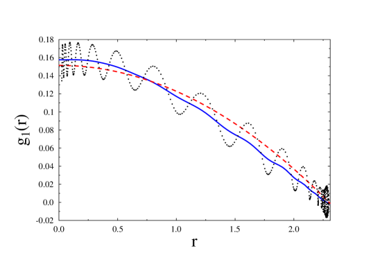
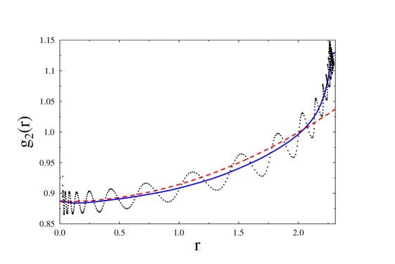
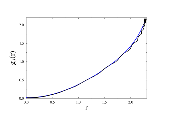
Figure 4: Blue solid lines: optimal reconstructions of the constitutive relations (a) $\hat{g}_{1}(r)$, (b) $\hat{g}_{2}(r)$ and (c) $\hat{g}_{3}(r)$. Red dashed lines: the corresponding initial guesses (a) $g^{0}_{1}(r)$ and (b) $g^{0}_{2}(r)$. Black symbols: values of (a) $r^{-1}\,(dr/dt)|_{r(t_{i})}$, (b) $(d\theta/dt)|_{r(t_{i})}$ and (c) $a_{\Delta}|_{r(t_{i})}$, computed based on the measurement data at the time instants $t_{i}$, $i=1,\dots,N_{T}$.

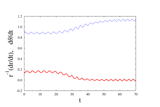
Figure 5: Dependence of the LHS in equations (2a)–(2b) evaluated based on the measurement data on time $t$. Red solid line: $r^{-1}\,(dr/dt)$. Blue dotted line: $(d\theta/dt)$.

Our main results are presented in Figure 4 where we show the optimal reconstructions $\hat{g}_{i}(r)$, $i=1,2,3$, and compare them against the left-hand sides of equations (2a)–(2c), all shown as functions of the state magnitude $r$. For completeness, the LHS of equations (2a)–(2b) are shown as functions of time $t\in[0,T]$ in Figure 5 (in the case of $\hat{g}_{1}$, cf. Figures 4a and 5, the LHS of equation (2a) is additionally divided into $r$). In Figures 4a,b we also indicate the RHS of mean-field model (34) which were used as the initial guesses for the reconstructions. We see in Figures 4 that, as expected, the reconstructed constitutive relations $\hat{g}_{i}(r)$, $i=1,2,3$, smoothly approximate the left-hand sides of the corresponding equations evaluated using the measurements. Considered as functions of $r$, these left-hand sides are multi-valued which is a consequence of the fact that, due to the oscillations of the measurement data at the limit cycle (see Figure 6a below), the map $t\rightarrow\tilde{r}(t)$ is not one-to-one. In Figures 4a,b we observe systematic deviations of the optimal reconstructions $\hat{g}_{1}$ and $\hat{g}_{2}$ from the corresponding functions in mean-field model (34). In addition, based on the reconstructions $\hat{g}_{1}$ and $\hat{g}_{2}$ we can obtain estimates of two important quantities, namely, the growth rate of the instability at the origin given by $\frac{d}{dr}\left[\hat{g}_{1}\,r\right]_{r=0}=\hat{g}_{1}(0)=0.1576$, and the oscillation frequency at the limit cycle given by $\hat{g}_{2}(r^{\circ})=1.130$. These numbers should be compared with, respectively, 0.151 and 1.036 obtained as discussed in Section 2.3 and used in mean-field model (34). Finally, in Figure 6 we compare the outputs from system (2) obtained using the mean-field model and the reconstructions $\hat{g}_{i}(r)$, $i=1,2,3$, against the corresponding measured quantities (as regards the time-history of the state variables, we do not show $a_{2}(t)$, as it has qualitatively very similar behavior to $a_{1}(t)$ already shown in Figure 6b). In Figures 6a,b (see, in particular, the insets) we note that the evolution of $r(t)$ and $a_{1}(t)$ obtained using the optimal reconstructions $\hat{g}_{1}$ and $\hat{g}_{2}$ is much closer to the measured quantities than the evolutions computed using mean-field model (34). We remark, however, that the measurements ${\tilde{r}}(t)$ shown in Figure 6a reveal some high-frequency oscillations which are not captured by the trajectory $r(t)$ obtained using the optimal reconstruction $\hat{g}_{1}$. These oscillations reflect a phase dependence in the behavior of the solutions of the original Navier-Stokes equation (5), an effect which is by construction excluded from ansatz (2a), cf. Assumption 1(a). As a consequence, $\hat{g}_{1}$ can convey phase-averaged information only. We will return to this problem again in Section 5.3. As regards the results shown in Figure 6c, we see that, while the optimal reconstruction $\hat{g}_{3}(r)$ is quite smooth (Figure 4c), the quantity $\hat{g}_{3}(r(t))$ exhibits oscillations absent in the original measurement data ${\tilde{a}}_{3}(t)$. This effect as well is a consequence of the lack of phase-dependence in ansatz (2a) and (2c).

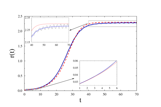
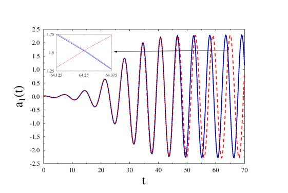
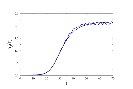
Figure 6: Comparison of (a) the state magnitude $r$, (b) state variable $a_{1}$ and (c) state variable $a_{3}$ as functions of time. Black dotted lines: measurement data. Blue solid lines: solution of system (2) using the optimal reconstructions $\hat{g}_{1}$, $\hat{g}_{2}$ and $\hat{g}_{3}$. Red dashed lines: solution of system (2) using initial guesses (34). In Figures (a) and (b) insets are included to highlight the differences between the data sets.

5 Discussion of Computational and Physical Aspects

In this Section we analyze a number of computational and physical modelling aspects of the proposed approach which can be important in applications. We begin by examining the accuracy of the cost functional gradients in Section 5.1, followed by a study of the robustness of iterations (17) in Section 5.2 and conclude with some insights about physical modelling in Section 5.3.

5.1 Validation of Gradients

A key element of optimization algorithm (17) are the cost functional gradients and a standard approach to their validation consists in computing the directional Gâteaux differential ${\mathcal{J}}^{\prime}_{i}(g_{i};g^{\prime}_{i})$, $i=1,2$, for some arbitrary perturbations $g^{\prime}_{i}$ in two different ways, namely, using a finite-difference approximation (with step size $\epsilon$) and using the inner product of the adjoint-based gradient with the perturbation $g^{\prime}_{i}$, namely Riesz representation (19), and then examining the ratio of the two quantities, i.e.,

$$\kappa_{i}(\epsilon):=\dfrac{\epsilon^{-1}\left[{\mathcal{J}}_{i}(g_{i}+\epsilon g^{\prime}_{i})-{\mathcal{J}}_{i}(g_{i})\right]}{\int_{{\mathcal{I}}}\bm{\nabla}^{L_{2}}{\mathcal{J}}_{i}(r)\,g^{\prime}_{i}(r)\,dr},\quad i=1,2,$$ (35)

for a range of values of $\epsilon$. If the gradient $\bm{\nabla}^{L_{2}}{\mathcal{J}}_{i}(r)$ is computed correctly, then for intermediate values of $\epsilon$, $\kappa_{i}(\epsilon)$ will be close to the unity. Remarkably, this behavior can be observed in Figures 7a,b corresponding to Problems $P1$ and $P2$ over a range of $\epsilon$ spanning about 8 orders of magnitude. The quantity shown in Figures 7a,b is $\log|\kappa_{i}(\epsilon)-1|$, $i=1,2$, which represents the number of significant digits to which the two ways to evaluate ${\mathcal{J}}^{\prime}_{i}(g_{i};g^{\prime}_{i})$ in (35) agree. Furthermore, we also observe that refining the resolution $N_{T}$ of the time interval $[0,T]$ yields values of $\kappa_{i}(\epsilon)$ closer to the unity. The reason is that in the “optimize-then-discretize” paradigm adopted here such refinement of the discretization leads to a better approximation of the continuous gradient (26). As can be expected, the quantities $\kappa_{i}(\epsilon)$ deviate from the unity for very small values of $\epsilon$, which is due to the subtractive cancellation (round-off) errors in finite-differencing, and also for large values of $\epsilon$, which is due to the truncation errors, both of which are well-known effects.

 

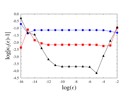
Figure 7: Diagnostic quantities (a) $\log|\kappa_{1}(\epsilon)-1|$ evaluated for Problem $P1$ and (b) $\log|\kappa_{2}(\epsilon)-1|$ evaluated for Problem $P2$, cf. (35), as functions of $\log\epsilon$ obtained using different discretizations of the time interval. Blue circles: $N_{T}=50$. Red squares: $N_{T}=500$. Black triangles: $N_{T}=5000$. In all cases the perturbation direction is $g^{\prime}_{i}=-r^{3}$, $i=1,2$.

5.2 Computational Robustness of the Proposed Approach

In this Section we focus on the effect that the choice of initial guess $g_{i}^{0}$, $i=1,2$, has on the reconstructed functions $\hat{g}_{1}$ and $\hat{g}_{2}$. We note that, given the nonlinearity of system (2), optimization problems $P1$ and $P2$ may be nonconvex and optimality conditions (16) and (27) characterize minimizers which are only local. Thus, different initial guesses may in principle give rise to different reconstructions and convergence to a global minimum cannot be a priori assured. We investigate this issue in Figures 9a and 9b where we show the reconstructions obtained, respectively, in Problems $P1$ and $P2$ using different initial guesses generally much worse than mean-field model (34) used in Section 4. As regards Problem $P1$, we note in Figure 9a that accurate reconstructions are obtained using even relatively poor initial guesses $g_{1}^{0}$. On the other hand, in Figure 9b we see that in Problem $P2$ the reconstruction fails for a less accurate initial guess $g_{2}^{0}$. These two examples are representative of the behavior we generally observed in our calculations and we conclude that Problem $P1$ appears more robust with respect to the choice of the initial guess than Problem $P2$. We also noted that in both problems convergence tends to be more sensitive to the values assumed by the initial guesses $g_{1}^{0}$ and $g_{2}^{0}$ at $r=0$ and $r=r^{\circ}$ than to their behavior for intermediate values of $r$. Results from Figure 9 are corroborated by the corresponding histories of the cost functionals in Figures 9a and 9b. We note that in the case of the poorest initial guess in Problem $P2$, cost functional ${\mathcal{J}}_{2}(g_{2}^{(n)})$ reveals hardly any decrease with the iterations at all. While in the cases of successful reconstructions the cost functionals ${\mathcal{J}}_{1}(g_{1}^{(n)})$ and ${\mathcal{J}}_{2}(g_{2}^{(n)})$ drop over several orders of magnitude, they never attain values lower than ${\mathcal{O}}(10^{-3})$. This is a consequence of the phase-dependent behavior of the measurements which cannot be resolved using ansatz in the form (2), cf. Assumption 1(a), see also the inset in Figure 6a.

   

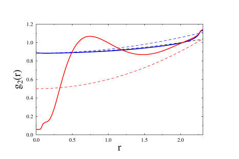
Figure 8: Reconstructions and the corresponding initial guesses in the solution of (a) Problem $P1$ and (b) Problem $P2$. Solid lines: reconstructions $\hat{g}_{i}$, $i=1,2$. Dashed lines: initial guesses $g_{i}^{0}$. Different reconstructions are marked with the same color as the corresponding initial guesses. Initial guesses and reconstructions discussed in Section 4 are marked in black.

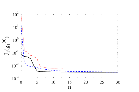
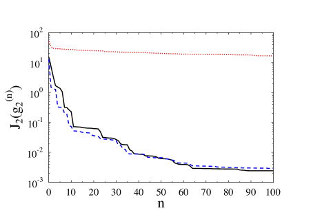
Figure 9: Decrease of the cost functionals with iterations in (a) Problem $P1$ and (b) Problem $P2$ for the cases studied in Figure 9 (with the same color-coding).

Inverse problems of the type considered here often tend to be ill-posed, in the sense that small perturbations to the data, for example due to noise, may result in significant changes in the computed solution. Suitable regularization, for instance, using Tikhonov’s technique [7, 30], may be required to stabilize the solution procedure in such situations. To focus attention in the present study, we concentrated on the structure of the gradients and did not investigate the effect of noise on the reconstructions, hence such regularization was not necessary. We refer the reader to [1, 2] for a thorough analysis of regularization applied to a related reconstruction problem.

5.3 Physical Interpretation of the Results

In this Section we propose some physical interpretation of the numerical reconstruction results from Section 4. We note in Figures 4 and 6 that the identified phase-invariant oscillation model (2) is in fact in remarkably good agreement with the data obtained from the solution of the Navier-Stokes equation (5). A small difference between the model and the data is visible as wiggles due to the second harmonic present in the measurements which violates the phase-invariance assumed in our model ansatz, cf. Assumption 1(a). This difference can be easily removed by a simple pre-processing of the measurement data. Referring to Appendix A, we note that the POD eigenvalue $\lambda_{1}$, representing the variance of $a_{1}$, is larger than the eigenvalue $\lambda_{2}$ which represents the variance of $a_{2}$. The following rescaling transformation

$${\bar{a}_{1}} = \sqrt{\frac{\lambda_{1}+\lambda_{2}}{2\lambda_{1}}}\>a_{1},$$ (36a)

$${\bar{a}_{2}} = \sqrt{\frac{\lambda_{1}+\lambda_{2}}{2\lambda_{2}}}\>a_{2}$$ (36b)

ensures equipartition of energy in the new variables $\bar{a}_{1}$ and $\bar{a}_{2}$ while conserving the total energy in both modes. This rescaling effectively removes the second harmonics from $\bar{a}_{i}$, $i=1,2$, which could be used as new inputs for the reconstruction. However, we refrained from applying (36) in the computations reported in Section 4 in order to show the power of the proposed identification method to deal with data which cannot be perfectly matched by the model.

Another observation concerning Figure 4 is the significant deviation of reconstructed functions $\hat{g}_{1}$ and $\hat{g}_{2}$ from the parabolic mean-field relations (8). Evidently, higher-order corrections, such as $r^{4}$, $r^{6}$, etc., are required for a better agreement between the identified propagators $\hat{g}_{i}$, $i=1,2$, and the expansions used in the mean-field model. The information which higher-order terms ought to be included in the model as opposed to an a priori fixed polynomial expansion used typically in model identification is therefore the unique advantage of the proposed identification strategy. We note that odd powers of $r$ can be excluded by phase-invariance considerations. In addition, with our reconstruction method we were able to determine more accurate values of the instability growth rate at the origin and the oscillation frequency at the limit cycle than used in mean-field model (34). We stress that in fact such seemingly insignificant modifications of the structure of the reduced-order model may already affect its utility for various control applications.

These results also shed light on the validity of mean-field model (8). Initially, the mean-field theory [37, 38] was derived to be valid near the onset of the oscillation only. We probed the applicability of this model by applying it at a Reynolds number $100$ which is more than twice the critical value of $47$. Hence, the deviation of $\hat{g}_{1}$ and $\hat{g}_{2}$ from (10) does not invalidate the mean-field theory. One reason for this deviation is the change of the structure of the vortex street during the transient. The optimal oscillatory modes deform from the stability eigenmodes into the POD modes while the fluctuation center moves upstream and the frequency and wavenumber increase [20, 39]. Similarly, the mean-field correction (the shift mode, cf. (7b)) changes during the transient [22] which has a noticeable effect on the mean-field model [40].

Finally, the results concerning the identified descriptor system are also relevant to the empirical 9-dimensional Galerkin model accounting for the base-flow variation and for the first four harmonics [20]. The initial exponential growth of the first harmonic is limited by the base-flow variation (which reduces the production of fluctuation energy) and, to a lesser extent, by the energy transfer from the first into higher harmonics. The energy transfer may be accounted for by an energy-dependent eddy viscosity in the mean-field system. Under certain assumptions (see, e.g. [41, chap. 3]), a generalized Landau equation

$$\dot{r}=\sigma_{1}r-\beta r^{3}-\gamma r^{3}$$ (37)

can be derived, where $\sigma_{1}$ denotes the growth rate near the fixed point $r=0$ and $\beta$, $\gamma$ characterize the damping from the $0$-th and from higher harmonics, respectively. By carefully comparing the 9-dimensional Galerkin model with the identified phase-invariant system it may be therefore possible to determine the values of $\beta$ and $\gamma$, or even to correct the powers of the new terms in (37). A complete derivation and an in-depth discussion of this problem is outside the scope of the present study.

6 Conclusions and Future Directions

We have proposed and validated a novel method for model identification which is an adaptation of an approach already used in the context of systems described by PDEs [1, 2]. As indicated in Figure 1, we depart from the traditional approach of (1) characterizing the propagator of the dynamical system in a parameter space and then (2) performing a parameter identification. Thus, arbitrary polynomial expansions of the propagator may be performed a posteriori (following the solution of the optimal reconstruction problem) at a practically vanishing cost. In addition, the performance of parametric models may easily be assessed and, if necessary, improved by introducing additional terms motivated by the form of the reconstructed constitutive relation.

The method is applied to a three-dimensional descriptor system with three a priori undetermined relations describing the fluctuation growth, frequency and mean-field correction as functions of the fluctuation energy. As a benchmark problem we chose the onset of laminar von Kármán vortex shedding behind a circular cylinder. Results of a direct numerical simulation are transcribed into the mode amplitudes of a minimal 3-state Galerkin model [20] which are then captured with remarkable accuracy by our identified descriptor system. The form of the reconstructed system is marked by a noticeable departure from the mean-field models and may therefore guide the refinement of the latter by inclusion of higher-order terms. We emphasize that the usefulness of reduced-order models for flow control applications may in fact depend on such differences.

As regards future research directions, while the present results offer a proof of the concept for the proposed approach based on a rather well-understood example, the key question is extension of this method to the identification of models with more complicated structure featuring, for example, multiple time scales, state space of a higher dimension, coexistence of several oscillation frequencies, non-trivial phase dependence and higher-dimensional inertial manifolds. As regards the first issue, one can consider a modification of our model problem (2)–(3) with Assumption 1(b) revised to allow $a_{3}(t)$ to be a “fast” variable. While in such setting our computational approach would formally remain unchanged (except that Problem $P3$ would be replaced with a problem similar to $P1$ or $P2$), it is interesting how it would actually perform in practice. Dealing with some of the other aspects will require formulation of the reconstruction problems in terms of propagator functions depending on more than just one state variable ($r$ in the examples considered in the present study). This will, in turn, lead to a number of interesting questions at the level of numerical analysis and scientific computing related to the evaluation of the cost functional gradients. An emerging application which involves some of the aforementioned extensions is related to the question of optimal parametrization of subgrid turbulence representations which is an important open problem in theoretical fluid mechanics [42]. In the context of Galerkin reduced-order models, it may take the form of an additional dissipative term with the magnitude proportional to an “eddy viscosity” $\nu_{T}$

$$\frac{d\bm{a}}{dt}=\bm{f}(\bm{a})+\nu_{T}\,{\bf L}^{\nu}\,\bm{a},\quad\bm{a}\in{\mathbb{R}}^{N},$$ (38)

where $\nu_{T}\,{\bf L}^{\nu}\,\bm{a}$ represents the stabilizing viscous term of the Navier-Stokes equation in the Galerkin system. In general, this term can be proven to be energy dissipative for all orthonormal systems of modes and a large class of boundary conditions. For some analytical modes, e.g., the Stokes modes, it can be shown that matrix ${\bf L}^{\nu}$ is diagonal and negative-definite. There is abundant evidence [41, 43, 44] that nonlinear closure strategies perform better as regards stabilization of system (38). Assuming $\nu_{T}=\nu_{T}(\|\bm{a}\|)$ gives rise to an identification problem analogous to $P1$ and $P2$, and one can use the algorithm described in Section 3 to determine optimal closure strategies leading to the best possible reconstruction of the available data. Preliminary identification results already obtained based on a reduced-order model (38) with dimension $N=20$ applied to a complex mixing-layer flow are quite encouraging and reveal some nontrivial physical insights. They will be reported in the near future upon completion of the study.

We also remark that a surprisingly large set of modelling and control problems can be cast in a similar form of function identification of a descriptor system

$$\frac{d\bm{a}}{dt}=\bm{f}(\bm{a},\bm{b}),\quad\bm{b}=\bm{g}(\bm{a}).$$ (39)

For reasons of simplicity, let us assume that function $\bm{f}$ is known and that function $\bm{g}$ needs to be determined. If $\bm{b}$ characterizes the slow modes, then $\bm{b}=\bm{g}(\bm{a})$ represents the inertial manifold to be identified from a given system trajectory [28]. If $\bm{b}$ represents high-frequency components, such as the parameters of a subgrid turbulence representation described above, then their functional dependence on the state variable $\bm{a}$ may also be inferred with our approach. On the other hand, if $\bm{b}$ denotes the actuation amplitudes, as in numerous wake flow stabilization studies [45, 46, 47, 48, 49], then $\bm{b}=\bm{g}(\bm{a})$ represents a full-state feedback control law. In principle, this control law may as well be identified from desired trajectories $t\mapsto\bm{a}(t)$.

Appendix A Proper Orthogonal Decomposition

In this Appendix we describe the Proper Orthogonal Decomposition (POD) employed in Section 2.2 to construct a low–dimensional model from the simulation data. It is closely related to other techniques of data analysis known as the Principal Component Analysis or, in the discrete setting, the Singular–Value Decomposition. The starting point are snapshots of the velocity field $\bm{u}^{m}(\bm{x}){:={\bm{u}}({\bm{x}},t^{m})}$, $m=1,\ldots,M$, $\bm{x}\in\Omega$, cf. (4). These snapshots are sampled at times $t^{m}$ uniformly spaced over one period of oscillation and form a statistically representative ensemble for the considered first and second moments.

The goal is to construct a ’least–order’ Galerkin expansion

$$\bm{u}(\bm{x},t)=\bm{u}_{0}(\bm{x})+\sum\limits_{i=1}^{N}a_{i}(t)\>\bm{u}_{i}(\bm{x})+\bm{u}_{\rm res}(\bm{x},t)$$ (40)

with base mode $\bm{u}_{0}$ and $N$ space-dependent expansion modes (basis functions) $\bm{u}_{i}(\bm{x})$ with the corresponding mode amplitudes $a_{i}(t)$ which will result in a minimum-norm average residual $\bm{u}_{\rm res}$ of the snapshot ensemble (see, e.g., [50, 41, 51]). The base mode is necessary so that Galerkin expansion (40) satisfies inhomogeneous boundary conditions for arbitrary mode amplitudes. For instance, expansion (40) captures the prescribed oncoming flow velocity regardless of the values of $a_{i}$.

The Galerkin expansion and its residual are embedded in the Hilbert space $L_{2}(\Omega)$ of square-integrable vector fields. The inner product of two elements $\bm{v},\bm{w}\in L_{2}(\Omega)$ is defined by

$${\big{\langle}\bm{v},\bm{w}\big{\rangle}_{{L_{2}(\Omega)}}:=\int\limits_{\Omega}\,\bm{v}\cdot\bm{w}\,d\bm{x}},$$ (41)

where ’$\cdot$’ denotes the standard Euclidean inner product and $d\bm{x}$ an infinitesimal volume element of the domain $\Omega$. The associated norm thus is

$$\|\bm{u}\|_{{L_{2}(\Omega)}}:=\sqrt{\langle\bm{u},\bm{u}\rangle_{{L_{2}(\Omega)}}}.$$ (42)

We search for empirical modes $\bm{u}_{i}$, $i=0,\ldots,N$, where $N\leq M-1$, which minimize the average residual of the Galerkin expansion of the snapshots

$$\bm{u}^{m}=\bm{u}_{0}+\sum\limits_{i=1}^{N}a_{i}^{m}\>\bm{u}_{i}+\bm{u}_{\rm res}^{m},\quad m=1,\ldots,M,$$ (43)

with optimal mode amplitudes $a_{i}^{m}$ in the sense of the $L_{2}$ norm, i.e.,

$$\overline{\left\|\bm{u}_{\rm res}\right\|^{2}_{{L_{2}(\Omega)}}}:=\frac{1}{M}\sum\limits_{m=1}^{M}\left\|\bm{u}_{\rm res}^{m}\right\|^{2}_{{L_{2}(\Omega)}}{=}\hbox{min}.$$ (44)

This problem is solved by the snapshot POD [52] and the base mode is the mean of the snapshots

$$\bm{u}_{0}:=\frac{1}{M}\sum\limits_{m=1}^{M}\bm{u}^{m}.$$ (45)

The POD modes arise from the correlation matrix $\bm{C}:=\left(C^{mn}\right)_{m,n=1,\ldots,M}$ of the snapshot fluctuations

$$C^{mn}:=\frac{1}{M}\Big{\langle}\bm{u}^{m}-\bm{u}_{0},\bm{u}^{n}-\bm{u}_{0}\Big{\rangle}_{{L_{2}(\Omega)}}.$$ (46)

We note that $\bm{C}$ is a positive semi-definite Grammian matrix. Hence, the eigenvalue problem

$$\bm{C}\bm{e}_{i}=\lambda_{i}\bm{e}_{i},\quad i=1,\ldots,M,$$ (47)

yields an orthonormal set of real eigenvectors $\bm{e}_{i}=\left[e_{i}^{1},\ldots,e_{i}^{M}\right]^{T}$, $\bm{e}_{i}^{T}\bm{e}_{j}=\delta_{ij}$, with non-negative eigenvalues which can be ordered as

$$\lambda_{1}\geq\lambda_{2}\geq\ldots\geq\lambda_{M}=0.$$ (48)

The last equality arises from the fact that $M$ vectors span a subspace of maximum dimension $M-1$. Hence, $M$ snapshots define only $M-1$ POD modes and the corresponding amplitudes. These are given by

$$\bm{u}_{i}=\frac{1}{\sqrt{M\lambda_{i}}}\sum\limits_{m=1}^{M}e_{i}^{m}\>\left(\bm{u}^{m}-\bm{u}_{0}\right),\quad a_{i}^{m}=\sqrt{\lambda_{i}M}\>e_{i}^{m},\quad i=1,\ldots,M-1.$$ (49)

The POD modes form an orthonormal basis in $L_{2}(\Omega)$, $\langle\bm{u}_{i},\bm{u}_{j}\rangle_{{L_{2}(\Omega)}}=\delta_{ij}$, $i,j=1,\ldots,N$, while their amplitudes have vanishing means $\overline{a_{i}}=0$, $i=1,\ldots,N$, and diagonal second moments $\overline{a_{i}\>a_{j}}=\lambda_{i}\>\delta_{ij}$, $i,j=1,\ldots,N$. The average is to be understood in terms of the snapshot ensemble (see, e.g., (44)). The eigenvalue $\lambda_{i}$ can be interpreted as twice the fluctuation energy contained the $i$-th mode.

Appendix B Regularity of Reconstructed Function $g_{1}$ versus Existence and Uniqueness of Solutions to Equation (2a)

By the one-dimensional embedding result $H^{1}({\mathcal{I}})\rightharpoonup C^{0,\frac{1}{2}}({\mathcal{I}})$ [35], we note that the reconstructed function will be Hölder-continuous with $\lambda=1/2$. Thus, it will not meet the assumptions of the Picard-Lindelöf theorem [53], and in principle will ensure existence only, without uniqueness, of solutions of equation (2a). In order to ensure the Lipschitz-continuity ($\lambda=1$) of $g_{1}$, which would also guarantee uniqueness of solutions of (2a), we would need to reconstruct $g_{1}$ as an element of Sobolev space $H^{2}({\mathcal{I}})$, because then $H^{2}({\mathcal{I}})\rightharpoonup C^{0,1}({\mathcal{I}})$. While there are no fundamental difficulties here (we would need to replace inner product (30) with the corresponding definition in $H^{2}({\mathcal{I}})$), we will refrain from this in the actual computations in Section 4 in order to keep the approach as simple as possible. Nevertheless, in all problems we treated with the proposed approach the reconstructed functions possessed the Lipschitz regularity which was verified a posteriori by performing suitable grid-refinement studies.

Appendix C Derivation of Perturbation Equation (20a)

In this Appendix we present a derivation of perturbation equation (20a). Obtaining this equation is made somewhat more involved by the fact that the perturbation variable $g_{1}$ is itself a function of the state magnitude, i.e., $g_{1}=g_{1}(r)$. We assume here that only $g_{1}$ is perturbed while $g_{2}$ remains fixed, with the opposite case leading to essentially the same calculations. By substituting, respectively, $g_{1}=g_{1a}$ and $g_{1}=g_{1b}$ into equation (3a), we obtain $\dot{\bm{\xi}}_{a}=\left(g_{1a}(r_{a})\,{\bf I}+g_{2}(r_{a})\,{\bf J}\right)\,\bm{\xi}_{a}$ and $\dot{\bm{\xi}}_{b}=\left(g_{1b}(r_{b})\,{\bf I}+g_{2}(r_{b})\,{\bf J}\right)\,\bm{\xi}_{b}$ , where $\bm{\xi}_{a}:=\bm{\xi}(g_{1a})$ and $\bm{\xi}_{b}:=\bm{\xi}(g_{1b})$ are the corresponding solutions and $r_{a}:=|\bm{\xi}_{a}|$, $r_{b}:=|\bm{\xi}_{b}|$. Taking the difference of these two equations and defining $\bm{\xi}^{\prime}:=\bm{\xi}_{a}-\bm{\xi}_{b}$. we obtain

$$\dot{\bm{\xi}}^{\prime} =g_{1a}(r_{a})\,{\bf I}\,\bm{\xi}_{a}+g_{2}(r_{a})\,{\bf J}\,\bm{\xi}_{a}-g_{1b}(r_{b})\,{\bf I}\,\bm{\xi}_{b}-g_{2}(r_{b})\,{\bf J}\,\bm{\xi}_{b}$$ (50)

$$=g_{1a}(r_{a})\,{\bf I}\,\bm{\xi}_{a}+g_{2}(r_{a})\,{\bf J}\,\bm{\xi}_{a}+g_{1b}(r_{a})\,{\bf I}\,\bm{\xi}_{a}-g_{1b}(r_{a})\,{\bf I}\,\bm{\xi}_{a}-g_{1b}(r_{b})\,{\bf I}\,\bm{\xi}_{b}-g_{2}(r_{b})\,{\bf J}\,\bm{\xi}_{b}$$

$$=g^{\prime}(r_{a})\,{\bf I}\,\bm{\xi}_{a}+\underbrace{g_{1b}(r_{a})\,{\bf I}\,\bm{\xi}_{a}-g_{1b}(r_{b})\,{\bf I}\,\bm{\xi}_{b}}_{A}+\underbrace{g_{2}(r_{a})\,{\bf J}\,\bm{\xi}_{a}-g_{2}(r_{b})\,{\bf J}\,\bm{\xi}_{b}}_{B},$$

where we also set $g^{\prime}(\cdot)=g_{1a}(\cdot)-g_{1b}(\cdot)$ in the first term on the RHS. As regards the terms denoted $A$ in (50), they are transformed as follows using the fundamental theorem of calculus for line integrals and the change of variables $\bm{\xi}(s)=\bm{\xi}_{b}+s\,(\bm{\xi}_{a}-\bm{\xi}_{b})$ for $s\in[0,1]$

$$A=g_{1b}(r_{a})\,{\bf I}\,\bm{\xi}_{a}-g_{1b}(r_{b})\,{\bf I}\,\bm{\xi}_{b} =\int_{\bm{\xi}_{b}}^{\bm{\xi}_{a}}\bm{\nabla}_{\bm{\xi}}(g_{1b}(\bm{\xi})\,\bm{\xi})\,d\bm{\xi}$$ (51)

$$=\left(\int_{0}^{1}\bm{\nabla}_{\bm{\xi}}{\bf F}(\bm{\xi}_{b}+s\bm{\xi}^{\prime})\,ds\right)\,\bm{\xi}^{\prime},$$

where we also denoted ${\bf F}(\bm{\xi}):=g_{1b}(\bm{\xi})\,\bm{\xi}$. The integrand expression on the RHS in (51) is then expanded in the Taylor series around $\bm{\xi}^{\prime}={\mathbf{0}}$

$${\partial\over\partial\xi_{j}}F_{i}(\bm{\xi}_{b}+s\bm{\xi}^{\prime})={\partial\over\partial\xi_{j}}F_{i}(\bm{\xi}_{b})+{\partial^{2}\over\partial\xi_{k}\,\partial\xi_{j}}F_{i}(\bm{\xi}_{b})\,\xi^{\prime}_{k}\,s+{\mathcal{O}}\left(|\bm{\xi}^{\prime}|^{2}\right),\quad i,j,k=1,2,$$ (52)

where the component notation was used for clarity with $F_{i}$, $\xi_{j}$ and $\xi^{\prime}_{k}$ denoting the components of vectors ${\bf F}$, $\bm{\xi}$ and $\bm{\xi}^{\prime}$. Plugging expansion (52) into expression (51) we obtain

$$A =\bm{\nabla}_{\bm{\xi}}(g_{1b}(\bm{\xi})\,\bm{\xi})\Big{|}_{\bm{\xi}=\bm{\xi}_{b}}\,\bm{\xi}^{\prime}\,\int_{0}^{1}\,ds+{\mathcal{O}}\left(|\bm{\xi}^{\prime}|^{2}\right)$$ (53)

$$=\left[g_{1b}(r_{b})\,{\bf I}+{\bf I}\,\bm{\xi}_{b}\,\left(\bm{\nabla}g_{1b}(r_{b})\right)^{T}\right]\,\bm{\xi}^{\prime}+{\mathcal{O}}\left(|\bm{\xi}^{\prime}|^{2}\right).$$

Noting that term $B$ in (50) transforms in an analogous way to $A$ in (51)–(53), using these results in (50), assuming smallness of $\bm{\xi}^{\prime}$ and dropping terms of order quadratic and higher we finally arrive at perturbation equation (20a).

References

- [1] V. Bukshtynov, O. Volkov, and B. Protas. On optimal reconstruction of constitutive relations. Physica D, 240:1228–1244, 2011.
- [2] V. Bukshtynov and B. Protas. Optimal reconstruction of material properties in complex multiphysics phenomena. Journal of Computational Physics, 242:889–914, 2013.
- [3] V. Bukshtynov. Computational Methods for the Optimal Reconstruction of Material Properties in Complex Multiphysics Systems. PhD thesis, McMaster University, 2012. Open Access Dissertations and Theses. Paper 6795. http://digitalcommons.mcmaster.ca/opendissertations/6795.
- [4] M. D. Gunzburger. Perspectives in Flow Control and Optimization. SIAM, 2003.
- [5] I. M. Navon. Practical and theoretical aspects of adjoint parameter estimation and identifiability in meteorology and oceanography. Dynamics of Atmosphere and Oceans, 27:55–79, 1997.
- [6] E. Kalnay. Atmospheric Modeling, Data Assimilation and Predictability. Cambridge University Press, 2003.
- [7] A. Tarantola. Inverse Problem Theory and Methods for Model Parameter Estimation. SIAM, 2005.
- [8] R. F. Stengel. Optimal Control and Estimation. Dover, 1994.
- [9] J.T. Stuart. Nonlinear stability theory. Ann. Rev. Fluid Mech., 3:347–370, 1971.
- [10] J. Dušek, P. Le Gal, and Ph. Fraunie. A numerical and theoretical study of the first Hopf bifurcation in a cylinder wake. Journal of Fluid Mechanics, 264:59, 1994.
- [11] L. D. Landau and E. M. Lifshitz. Statistical Physics. Pergamon Press, 1980.
- [12] I. R. Yukhnovskii. Phase Transitions of the Second Order — Collective Variables Method. World Scientific, 1987.
- [13] C.P. Jackson. A finite-element study of the onset of vortex shedding in flow past variously shaped bodies. J. Fluid Mech., 182:23–45, 1987.
- [14] M. Morzyński, K. Afanasiev, and F. Thiele. Solution of the eigenvalue problems resulting from global non-parallel flow stability analysis. Comput. Meth. Appl. Mech. Enrgrg., 169:161–176, 1999.
- [15] B. R. Noack and H. Eckelmann. A global stability analysis of the steady and periodic cylinder wake. J. Fluid Mech., 270:297–330, 1994.
- [16] C.W. Rowley and D.R. Williams. Dynamics and control of high-Reynolds number flows over open cavities. Ann. Rev. Fluid Mech., 38:251–276, 2006.
- [17] P. J. Schmid and D. S. Hennigson. Stability and Transition in Shear Flows. Springer-Verlag, New York, 2001.
- [18] A. Zebib. Stability of viscous flow past a circular cylinder. J. Engr. Math., 21:155–165, 1987.
- [19] H.-Q. Zhang, U. Fey, B. R. Noack, M. König, and H. Eckelmann. On the transition of the cylinder wake. Phys. Fluids, 7(4):779–795, 1995.
- [20] B. R. Noack, K. Afanasiev, M. Morzyński, G. Tadmor, and F. Thiele. A hierarchy of low-dimensional models for the transient and post-transient cylinder wake. J. Fluid Mech., 497:335–363, 2003.
- [21] P. Holmes, J. L. Lumley, and G. Berkooz. Turbulence, Coherent Structures, Dynamical Systems and Symmetry. Cambridge University Press, 1996.
- [22] G. Tadmor, O. Lehmann, B. R. Noack, and M. Morzyński. Mean field representation of the natural and actuated cylinder wake. Phys. Fluids, 22(3):034102–1..22, 2010.
- [23] A. E. Deane, I. G. Kevrekidis, G. E. Karniadakis, and S. A. Orszag. Low-dimensional models for complex geometry flows: Application to grooved channels and circular cylinders. Phys. Fluids A, 3:2337–2354, 1991.
- [24] W.V.R. Malkus. Outline of a theory of turbulent shear flow. J. Fluid Mech., 1:521–539, 1956.
- [25] D. Barkley. Linear analysis of the cylinder wake mean flow. Europhysics Lett., 75:750–756, 2006.
- [26] H. Haken. Synergetics, An Introduction. Nonequilibrium Phase Transitions and Self-Organizations in Physics, Chemistry, and Biology. Springer, New York, 3rd edition, 1983.
- [27] J. Guckenheimer and P. Holmes. Nonlinear Oscillations, Dynamical Systems, and Bifurcation of Vector Fields. Springer, New York, 1986.
- [28] A. N. Gorban and I. V. Karlin. Invariant Manifolds for Physical and Chemical Kinetics. Number Vol. 660 in Lecture Notes in Physics. Springer-Verlag, Berlin, 2005.
- [29] G. Chavent and P. Lemonnier. Identification de la non–linearité d’une équation parabolique quasilineaire. Applied Mathematics and Optimization, 1:121–162, 1974.
- [30] C. R. Vogel. Computational Methods for Inverse Problems. SIAM, 2002.
- [31] D. Luenberger. Optimization by Vector Space Methods. John Wiley and Sons, 1969.
- [32] W. H. Press, B. P. Flanner, S. A. Teukolsky, and W. T. Vetterling. Numerical Recipes: the Art of Scientific Computations. Cambridge University Press, 1986.
- [33] J. Nocedal and S. Wright. Numerical Optimization. Springer, 2002.
- [34] M. S. Berger. Nonlinearity and Functional Analysis. Academic Press, 1977.
- [35] R. A. Adams and J. F. Fournier. Sobolev Spaces. Elsevier, 2005.
- [36] B. Protas, T. Bewley, and G. Hagen. A comprehensive framework for the regularization of adjoint analysis in multiscale pde systems. Journal of Computational Physics, 195:49–89, 2004.
- [37] J.T. Stuart. On the non-linear mechanics of hydrodynamic stability. J. Fluid Mech., 4:1–21, 1958.
- [38] J. Watson. On the non-linear mechanics of wave disturbances in stable and unstable parallel flows. Part 2. the development of a solution for plane Poiseuille flow and for plane Couette flow. J. Fluid Mech., 9:371–389, 1960.
- [39] G. Tadmor, O. Lehmann, B. R. Noack, L. Cordier, J. Delville, J.-P. Bonnet, and M. Morzyński. Reduced order models for closed-loop wake control. Philosophical Transactions of the Royal Society A, 369(1940):1513–1524, 2011.
- [40] M. Morzyński, W. Stankiewicz, B. R. Noack, F. Thiele, and G. Tadmor. Generalized mean-field model for flow control using continuous mode interpolation. In 3rd AIAA Flow Control Conference, San Francisco, Ca, USA, 5-8 June 2006, 2006. Invited AIAA-Paper 2006-3488.
- [41] B. R. Noack, M. Morzyński, and G. Tadmor (eds.). Reduced-Order Modelling for Flow Control. Number 528 in CISM Courses and Lectures. Springer-Verlag, Berlin, 2011.
- [42] J. A. Langford and R. D. Moser. Optimal LES formulations for isotropic turbulence. Journal of Fluid Mechanics, 398:321–346, 1999.
- [43] Z. Wang, I. Akhtar, J. Borggaard, and T. Iliescu. Proper orthogonal decomposition closure models for turbulent flows: A numerical comparison. Comput. Methods Appl. Mech. Engrg., 237-240:10–26, 2012.
- [44] M. Balajewicz, E. H. Dowell, and B. R. Noack. Low-dimensional modelling of high-Reynolds-number shear flows incorporating constraints from the Navier-Stokes equation. J. Fluid Mech., 729:285–308, 2013.
- [45] J. Gerhard, M. Pastoor, R. King, B. R. Noack, A. Dillmann, M. Morzyński, and G. Tadmor. Model-based control of vortex shedding using low-dimensional Galerkin models. In 33rd AIAA Fluids Conference and Exhibit, Orlando, Florida, USA, June 23–26, 2003, 2003. Paper 2003-4262.
- [46] M. Bergmann, L. Cordier, and J.-P. Brancher. Optimal rotary control of the cylinder wake using proper orthogonal decomposition reduced order model. Phys. Fluids, 17:097101–121, 2005.
- [47] B. Thiria, S. Goujon-Durand, and J. E. Wesfreid. The wake of a cylinder performing rotary oscillations. J. Fluid Mech., 560:123–147, 2006.
- [48] M. Pastoor, L. Henning, B. R. Noack, R. King, and G. Tadmor. Feedback shear layer control for bluff body drag reduction. J. Fluid Mech., 608:161–196, 2008.
- [49] J. Weller, E. Lombardi, and A. Iollo. Robust model identification of actuated vortex wakes. Physica D, 238:416–427, 2009.
- [50] C. A. J. Fletcher. Computational Galerkin Methods. Springer, New York, 1st edition, 1984.
- [51] P. Holmes, J. L. Lumley, G. Berkooz, and C. W. Rowley. Turbulence, Coherent Structures, Dynamical Systems and Symmetry. Cambridge University Press, Cambridge, 2nd paperback edition, 2012.
- [52] L. Sirovich. Turbulence and the dynamics of coherent structures, Part I: Coherent structures. Quart. Appl. Math., XLV:561–571, 1987.
- [53] R. K. Miller and A. N. Michel. Ordinary Differential Equations. Academic Press, 1982.