Gamma-ray active galactic nuclei type determination through machine-learning algorithms

Abstract

The Fermi Gamma-ray Space Telescope (Fermi) is producing the most detailed inventory of the gamma-ray sky to date. Despite tremendous achievements approximately 25% of all Fermi extragalactic sources in the Second Fermi LAT Catalogue (2FGL) are listed as active galactic nuclei (AGN) of uncertain type. Typically, these are suspected blazar candidates without a conclusive optical spectrum or lacking spectroscopic observations. Here, we explore the use of machine-learning algorithms – Random Forests and Support Vector Machines – to predict specific AGN subclass based on observed gamma-ray spectral properties. After training and testing on identified/associated AGN from the 2FGL we find that 235 out of 269 AGN of uncertain type have properties compatible with gamma-ray BL Lacs and flat-spectrum radio quasars with accuracy rates of 85%. Additionally, direct comparison of our results with class predictions made after following the infrared colour-colour space of Massaro et al. (2012) shows that the agreement rate is over four-fifths for 54 overlapping sources, providing independent cross validation. These results can help tailor follow-up spectroscopic programmes and inform future pointed surveys with ground-based Cherenkov telescopes.

1 Introduction

The Fermi mission has revolutionised our knowledge of high-energy gamma ray sources in the 100 MeV to 100 GeV energy range. Instrumentally, the Large Area Telescope (LAT) increased sensitivity and sky coverage represents a giant leap forward compared to EGRET (Hartman et al., 1999), allowing access to the gamma-ray sky with unprecedented detail. With over two years of collected data, the Second Fermi LAT Catalogue (2FGL) lists a total of 1873 point-like sources, including 1092 objects connected with known AGN at other wavelengths (Abdo et al., 2011; Ackermann et al., 2011).

Out of the 1092 sources designated as AGN, 436 are BL Lacertae objects (BL Lacs), 370 are flat-spectrum radio quasar (FSRQs), 12 are radio galaxies, 6 are Seyferts and 11 are other AGN. Despite this important level of achieved sophistication, the remaining 257 sources are designated as active galaxies of uncertain type (AGU) that total 25% of all AGN. Generally, AGU are positionally coincident with flat-spectrum radio sources showing distinctive broad-band blazar characteristics, but lacking reliable optical measurements (Ackermann et al., 2011).

In order to understand all the intricacies of the AGN population, it is important to take further steps to assess the nature and redshift of the sources classified as AGU. In the past, this has been accomplished via a two-step approach. The initial classification of an AGN relies on painstakingly dedicated optical spectroscopy to help identify unique emission or absorption features (Shaw et al., 2009). If no significant features are found, the second step consists of multi-band photometry to help estimate the redshift of suspected BL Lacs (Sbarufatti, Treves & Falomo, 2005; Meisner & Romani, 2010; Rau et al., 2012).

Without optical spectroscopy, one generally does not have sufficient information to determine directly whether an individual source is a BL Lac or a FSRQ. Unfortunately, optical spectral observations are taxing and can take years to complete. Ideally, one would like to find a discriminator for distinct source subclasses that relies solely on readily available observational characteristics. Recently, Massaro et al. (2012) introduced a method that helps recognise gamma-ray blazar subclass based on infrared colours from the Wide-Field Infrared Survey Explorer (WISE). Here, we explore the possibility of determining AGN subclass for Fermi sources directly from gamma-ray spectral features extracted from the 2FGL.

In particular, we present results from supervised machine learning algorithms, Random Forests and Support Vector Machines, that are initially trained on identified/associated AGN and subsequently used to infer specific blazar subclass of AGN of uncertain type. This is a natural extension of previous machine-learning strategies introduced to predict source class in unassociated Fermi point sources (Ackermann et al., 2012a; Mirabal et al., 2012; Lee et al., 2012). In Section 2 we describe the machine learning algorithms. The procedure used to train and test the algorithms is summarised in Section 3, including feature selection and creation of datasets. Individual predictions for AGU as well as an extension to unassociated Fermi sources are presented in Section 4. Finally, we compare our predictions with Massaro et al. (2012) and provide conclusions in Section 5.

2 Classification algorithms

The improvement and application of supervised learning algorithms has become a central part of the exploration of astrophysical data in a variety of contexts, ranging from object characterisation (Ball et al., 2006; Ackermann et al., 2012a; Mirabal et al., 2012) to variability (Richards et al., 2012). In this paper, we employ Support Vector Machines (SVMs) and Random Forests (RF) that embody two of the most robust supervised learning algorithms available today (Bloom & Richards, 2011). Brief descriptions of both algorithms are given in this section. Both RF and SVMs have been extensively described in the literature (Vapnik, 1995; Breiman, 2001).

2.1 Support Vector Machines

Support Vector Machines (SVMs) have proven to be one of the most effective supervised learning algorithms for pattern recognition (Vapnik, 1995; Cortes & Vapnik, 1995). The underlying rationale behind the algorithm seeks to find the optimal margin classifier by constructing a separating hyperplane that divides the training set and maximises the separation between different classes, which can then be used either in classification or regression analysis.

The points lying closer to the boundaries of a certain hyperplane are called support vectors. The latter determine the minimum distances between the hyperplane and their respective classes, the so called margin. The maximisation of the optimal margin is computed by taking into account only these vectors, the most representative points to construct the classifier. Complex separating surfaces can be introduced through the use of kernel functions, which transform the problem into a linear one in a higher-dimensional space. Polynomial, gaussian or radial plane kernel functions are often used. SVMs excel in performance handling high-dimensional data that can also incorporate the trade off between training errors and overall margins parametrized by a scaling factor $\gamma$ and error penalty $C$.

The analysis presented in this work was performed under the R programming language. Specifically, we adopted the e1071 package as the interface to libsvm (Chih-Chung & Chih-Jen, 2011). This offers a very fast and efficient SVM application with the option for automatically tuning parameters to the data and the use of different kernel functions.

2.2 Random Forests

Random Forests is an ensemble classifier that grows a large forest of classification trees that independently make class estimation (Breiman, 2001). Each decision tree selects a number of random input features and creates the best split based on a out-of-bag (oob) random selected set of the whole training data sample. Once the decision forest is built, decision thresholds are computed by counting the votes after running the oob datasets through every tree.

A RF classifier is ideal for data mining and variable selection as it incorporates efficient ways of calculating feature importance in the training set. This is achieved by replacing features across classification trees with random values and quantifying the effect of the changes. If the result of the decisions does not change significantly after these changes, the feature has a relatively low importance. On the other hand, if the accuracy rates change dramatically, a particular feature is deemed as important. There is no need for cross-validation with a separate testing set as the process itself computes accuracy rate internally.

In this work we used the randomForest package (Liaw & Wiener, 2002), which adapts the original Random Forests (Breiman, 2001) for classification and regression to the R language. randomForest provides excellent macros for plotting and tuning. Recently, Mirabal et al. (2012) introduced Sibyl a successful classifier that uses Random Forests to predict source class for unassociated Fermi sources based on 2FGL features and it serves as the principal formulation for our analysis.

3 PROCEDURE

Before delving into a formal application of the algorithms, datasets must be carefully extracted from the 2FGL and both SVMs and RF must be tuned to achieve their best performance.

 

Figure 1: Distributions of Powerlaw Index (left) and Pivot Energy (right) for identified/associated BL Lacs (black) and FSRQs (grey). The filled areas show results for AGU: Predicted BL Lacs (filled dark area) and predicted FSRQs (filled light area).

3.1 Construction of the datasets

For a proper use of supervised learning algorithms, we need to explore the feature space in order to find out the variables that best capture each class we want to determine. In this case, we are interested in building classifiers that can distinguish between two AGN classes: BL Lacs and FSRQs. In the 2FGL, there are a total set of 1074 identified/associated AGN objects with the following labels: “bzb” (BL Lacs), “bzq” (FSRQs), “agn”(other non-blazar AGN) and “agu” (active galaxies of uncertain type). From this global set, we group the identified/associated blazars (“bzb” and “bzq” labels) as the training/testing set of our algorithms. We end up with a set of 806 sources, divided in a fairly balanced manner that includes 370 FSRQs and 436 BL Lacs. In addition, we place all the undetermined sources (“agu” labels) in a separate dataset consisting of the 257 objects. Once the algorithms are trained and tested, we will apply the classifiers to the latter. Note that we will initially approach our study as a simple binary classification problem that attempts to distinguish whether an individual AGU is a BL Lac or a FSRQ. It is possible that other subclasses are represented within the AGU dataset. However, additional AGN subclasses only account for 3% of the whole AGN sample. Nevertheless, we will discuss the effects of additional complexity later on.

3.2 Feature selection

The next step involves choosing from the different gamma-ray spectral features available for each source. Although the algorithms are not strongly affected by noise, it is relevant to limit misleading features that might affect the characterisation. Initially, we select all basic features reported in the 2FGL (Abdo et al., 2011). As in Mirabal et al. (2012), we supplement these with Hardness Ratios ($HR_{i}={Flux_{i}-Flux_{j}}/{Flux_{i}+Flux_{j}}$) and Flux Ratios ($FR_{ij}=Flux_{i}/Flux_{j}$), ending up with a set of 20 distinct features. Armed with this set of variables, we compute feature importance to find those most representative with a robust method already implemented in the randomForest package (Liaw & Wiener, 2002; Mirabal et al., 2012). This process outputs two measures of importance: MeanDecreaseAccuracy and MeanDecreaseGini. Both are excellent indicators of feature relevance (Breiman, 2001).

Once feature importance measures are computed, we create new sets of data with different number of features by iteratively removing the variables with lower MeanDecreaseAccuracy, and comparing accuracy rates attained by RF and SVM algorithms on these sets. Although RF does not require a tailored training/testing analysis to estimate accuracy rates, it is useful to compare both algorithms directly with identical training/testing sets. Through feature selection, we downsize the initial 20 features to a final set of 9. The final set of variables includes (ordered by decreasing MeanDecreaseGini) Powerlaw Index (76.6), Pivot Energy (59.2), Flux Density (27.1), Variability Index (20.1), Flux1000 (12.6), and four Hardness Ratios: $HR_{2}$ (19.4), $HR_{1}$ (17.5), $HR_{3}$ (14.4) & $HR_{4}$ (10.6). Features considered but later discarded include Spectral Index, Energy Flux, Curvature Index, Flux in five different energy ranges, and Flux Ratios.

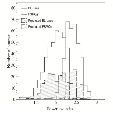
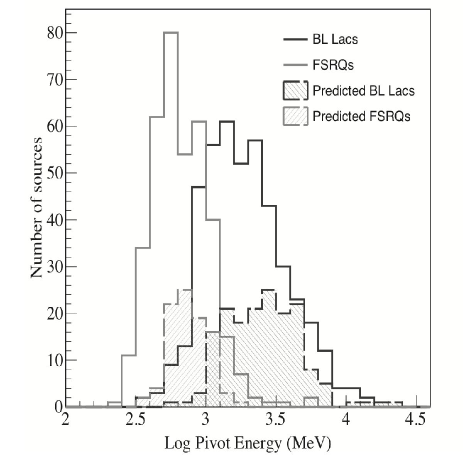
The top two most representative features for AGN subclass determination are Powerlaw Index and Pivot Energy. The clean separation between blazars is obvious in Fig. 1 and it intuitively stands on observational arguments. As explained in Ackermann et al. (2011), there is a well established spectral difference in the LAT energy range between FSRQs and BL Lacs. In general, the AGN inverse Compton (IC) peak is located at lower energies for FSRQs and at higher energies for BL Lac objects. Typical values are 1 MeV – 1 GeV for FSRQ and 100 MeV – 100 GeV for BL Lacs respectively (Abdo et al., 2010b).

The overall effect is that FSRQs show softer spectra than BL Lacs, and therefore, higher values of Powerlaw Index. Pivot Energy is defined as the energy at which the relative uncertainty on the differential flux is minimal. It is also an estimate of the point where the covariance of Powerlaw Index and Flux Density is minimised (Abdo et al., 2011). The relative dominance of lower energy events for FSRQs places the general location of the Pivot energy at lower energies compared to BL Lac spectra. As a result, the difference found in Pivot Energy between both populations can be understood as the overall effect of the spectral characteristics of FSRQs and BL Lacs produced by the difference on the position of IC peak in the spectral energy distribution for both populations.

3.3 Tuning, training and testing

Both SVM and RF algorithms require parameter tuning to achieve their best performance. In the case of SVMs, there is an automatic tuning process best.tune that returns the appropriate values of $C$ and $\gamma$ for a particular kernel function and training set. In order to make a selection, we scanned the classification accuracies for different kernel functions and used the tuned parameters to discriminate amongst them. Linear, polynomial, sigmoid, and radial kernels were tested. For the final training set, we settled on a C-classification linear kernel with $C=1$ and $\gamma=0.11$. For RF, tuneRF() performs an automatic search for the most efficient number of features used per classification tree for a chosen training set (Liaw & Wiener, 2002). Ultimately, we employ 9 spectral features, four variables randomly sampled at each split, and a total of 5000 trees.

After culling our datasets with the chosen features and tuning the algorithms for best performance, testing is performed to estimate the error of the resulting classification. As training set, we use a random selection of $2/3$ of all identified/associated AGN and the remaining $1/3$ is used as a testing set. To estimate the accuracy rates, we compare the actual source class with the class predicted by each classifier. For 500 of these training and testing sets, we obtain average accuracy rates of $85\%$, adopting a decision threshold of $P>0.5$ for both RF and SVMs. Note that with such threshold there are few ambiguous events since we require both $P_{SVM}$ and $P_{RF}$ must be greater than 0.5. If we consider a more conservative condition, for instance $P>0.8$, the accuracy rates improve to $94\%$. In this case, there is a bigger fraction of the sample that remains untagged.

For further verification, we also computed rates by leaving one object out from the training set and using that single object as the testing set. The leave-one-out cross validation rate is $85\%$ for common decision threshold of $P>0.5$ and $95\%$ with $P>0.8$ showing that larger training sets do not produce significant increases in accuracy rates.

4 Results

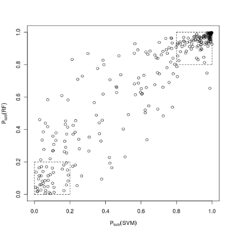
Once the classifiers have been trained and tested, we apply both algorithms to the set of AGN of uncertain type. For each of the 257 AGU, the classifiers returns a decision threshold that an individual object is a BL Lac ($P_{bzb}$) or a FSRQ ($P_{bzq}$), where $P_{bzq}=1-P_{bzb}$. A fraction of the resulting predictions is listed in Table 1. Decision thresholds $P_{bzb}$ calculated with both RF and SVMs are shown, as well as a class prediction satisfying the condition $P(RF)$ and $P(SVM)>0.8$. In Fig. 2 we plot $P(RF)$ and $P(SVM)$ obtained with each classifier for the 257 sources. Overall, there is an agreement rate of 91% between the algorithms. Though there are some discrepancies (for instance RF show higher BL Lac classification rates than SVMs), the results are outstanding considering the distinct underlying assumptions of the algorithms.

Figure 2: Decision threshold $P_{bzb}$ obtained with RF versus $P_{bzb}$ estimated by SVM for 257 AGU in the 2FGL. Dashed squares contain sources with common decision threshold over 0.8, classified with accuracy rates over 94%.

Table 1: Predictions for Fermi AGN of uncertain type in the 2FGL, ordered by RA. Threshold values $P_{bzb}<$ 0.2 (in the case of FSRQs) and $P_{bzb}>$ 0.8 (in the case of BL Lacs) must be met in both methods.

Source	$P_{bzb}$ (RF)	$P_{bzb}$ (SVM)	Prediction
2FGL J0001.7-4159	0.84	0.80	bzb
2FGL J0009.1+5030	0.97	0.95	bzb
2FGL J0009.9-3206	0.53	0.57	-
2FGL J0010.5+6556c	0.14	0.07	bzq
2FGL J0018.8-8154	0.69	0.80	-
2FGL J0019.4-5645	0.16	0.04	bzq
2FGL J0022.2-1853	0.99	1.00	bzb
2FGL J0022.3-5141	0.46	0.50	-
2FGL J0038.7-2215	0.99	1.00	bzb
2FGL J0044.7-3702	0.06	0.04	bzq
2FGL J0045.5+1218	0.91	0.85	bzb
2FGL J0051.4-6241	1.00	1.00	bzb
2FGL J0055.0-2454	1.00	0.99	bzb
2FGL J0056.8-2111	0.97	0.99	bzb
2FGL J0059.2-0151	0.95	0.99	bzb
2FGL J0059.7-5700	0.03	0.02	bzq
2FGL J0103.5+5336	0.93	0.94	bzb
2FGL J0110.3+6805	0.86	0.68	-
2FGL J0118.6-4631	0.96	0.98	bzb
2FGL J0127.2+0324	0.98	0.99	bzb
2FGL J0131.1+6121	0.93	0.97	bzb
2FGL J0134.4+2636	0.99	0.97	bzb
2FGL J0137.7+5811	0.44	0.38	-
2FGL J0146.6-5206	0.95	0.92	bzb

Note: The complete list of predictions is available at http://www.gae.ucm.es/~thassan/agus.html.

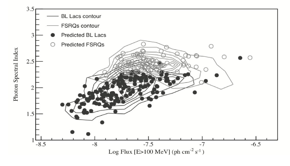
Table 2 shows overall numbers sorted according to different criteria imposed for both RF and SVM. In particular we list the predicted number of occurrences in terms of different decision thresholds ($P>$ 0.5, 0.8, and 0.95). We include individual algorithms and coincidences, satisfying said conditions. Combining results from both classifiers and requiring $P>0.5$, 235 (156 BL Lacs and 79 FSRQs) out of 257 objects are consistent with the properties of known gamma-ray blazars. In order to place these results in context with identified/associated Fermi AGN, Fig. 3 shows the photon spectral index versus the flux ($E>$ 100 MeV) of identified/associated BL Lacs and FSRQs overlaid with the AGU predictions from this work.

Table 2: Number of predicted AGU sources as a function of decision threshold.

	RF		SVMs		Both
	bzb	bzq	bzb	bzq	bzb	bzq
$P>0.5$	173	84	161	96	156	79
$P>0.8$	129	46	112	63	106	39
$P>0.95$	64	12	64	19	47	5

Figure 3: Photon spectral index versus log flux above 100 MeV for identified/associated BL Lacs (dark contour) and FSQRs (light contour). Predicted BL Lacs (filled circles) and predicted FSRQs (open circles) from the AGU dataset are shown over the contours.

4.1 Outlier detection and potential biases

Throughout, we have assumed that the classification of gamma-ray AGN subclass falls along the two main blazar categories i.e. BL Lacs and FSRQs. Without final spectroscopy it is impossible to rule that other AGN subclasses are present in the AGU sample. As commented before, there is a minority of other subclasses in the 2FGL including Seyferts, radio galaxies and other AGN that have not been considered thus far. The main justification for ignoring further atomisation into subclasses is that blazars account for 97% of the identified/associated AGN sample. However, it is important to consider that a more complex mixture of AGN subclasses is possible. Fortunately, machine-learning algorithms excel at separating rare and unique objects from the dataset.

Adopting the method introduced in Mirabal et al. (2012), we performed a search for AGU outliers that could potentially belong to other minority AGN subclasses. For this purpose, we computed the outlying measure of each object defined as the reciprocal sum of the squared proximities to all objects within its class. Outliers are defined as objects having small proximities to the rest of objects. Practically, RF returns proximities $prox(n,k)$ that represent the fraction of trees in which elements $n$ and ${k}$ fall in the same terminal node (Breiman, 2001; Liaw & Wiener, 2002). Generally, anomalies are identified with outlier measures larger than 10. No source was found with such values, as a result we conclude that there is no clear evidence of outliers in the AGU dataset. For completeness, we note that the highest values in the dataset correspond to 2FGL J1825.1–5231, 2FGL J1816.7–4942, and 2FGL J0022.3–5141 respectively.

We constrained this possibility further by retraining and testing the SVMs and RF algorithms with the full range of associated AGN subclasses present in the 2FGL. Given the size of the minority subclasses, care was taken to weight the classes appropriately to compensate the differences in the training sets (Mirabal et al., 2012). Taking into account additional AGN subclasses, we find that at most 11 objects might belong to other AGN subclasses ($P<$ 0.6). Therefore, there is no strong indication of contamination from additional subclasses. Taken together, both approaches limit the presence of other AGN subclasses in the AGU dataset. It is possible that the result simply reflects the small number statistics of additional AGN subclasses. A full characterization might improve in the future as Fermi expands its source catalogue.

4.2 Application to unassociated Fermi objects

In Mirabal et al. (2012), we introduced class predictions for the sample of unassociated Fermi sources at $|b|\geq 10^{\circ}$. In that initial approach, we simply considered sorting sources in broad AGN and pulsar categories. Given our success with further AGN subclasses, it is interesting to extend the approach to all unassociated Fermi sources tagged as AGN. Using the same optimised models, we apply the algorithms to the 216 sources predicted as AGN in Mirabal et al. (2012). The resulting predictions are shown in Table 3 with the same conditions adopted earlier. In this case, only 30% of the sources reach decision thresholds larger than $P>$ 0.8 in both RF and SVM.

Table 3: Predictions for unassociated Fermi objects tagged as AGN by Mirabal et al. (2012), ordered by RA.

Source	$P_{bzb}$ (RF)	$P_{bzb}$ (SVM)	Prediction
2FGL J0004.2+2208	0.15	0.11	bzq
2FGL J0014.3-0509	0.37	0.19	-
2FGL J0031.0+0724	0.97	0.94	bzb
2FGL J0032.7-5521	0.41	0.28	-
2FGL J0039.1+4331	0.87	0.99	bzb
2FGL J0048.8-6347	0.91	0.76	-
2FGL J0102.2+0943	0.90	0.89	bzb
2FGL J0103.8+1324	0.94	0.95	bzb
2FGL J0116.6-6153	0.97	0.99	bzb
2FGL J0124.6-2322	0.49	0.66	-
2FGL J0129.4+2618	0.19	0.05	bzq
2FGL J0133.4-4408	0.63	0.73	-
2FGL J0143.6-5844	1.00	0.99	bzb
2FGL J0158.4+0107	0.36	0.26	-
2FGL J0158.6+8558	0.06	0.07	bzq
2FGL J0200.4-4105	0.98	0.99	bzb
2FGL J0221.2+2516	0.99	0.99	bzb
2FGL J0226.1+0943	0.66	0.76	-
2FGL J0227.7+2249	0.89	0.95	bzb
2FGL J0239.5+1324	0.99	0.95	bzb
2FGL J0251.0+2557	0.37	0.19	-
2FGL J0305.0-1602	0.99	1.00	bzb
2FGL J0312.5-0914	0.93	0.69	-
2FGL J0312.8+2013	0.91	0.97	bzb

Note: The complete list of predictions is available at http://www.gae.ucm.es/~thassan/agus.html.

5 Discussion and Conclusions

We have used RF and SVM classifiers to predict specific source subclasses for gamma-ray AGN of uncertain type, by learning from features extracted from associated AGN in the 2FGL. Both algorithms are extremely successful in capturing the properties of gamma-ray AGN reaching accuracy rates of 85%. This effort allows us to show that 235 out of 269 AGN of uncertain type have properties consistent with gamma-ray BL Lacs and FSRQs, with decision thresholds over 0.8. Comparison of these predictions with the sample of associated AGN verify that we are indeed tracing similar populations (Fig. 3). Nevertheless, without high-quality spectral observations, final counterpart association will have to wait for dedicated optical spectroscopy.

Apart from internal training and testing, we can cross-match our results with a recent study showing that blazars can be recognised and separated from other extragalactic sources using infrared colours (Massaro et al., 2012). Class characterisation has been done for Fermi AGN of uncertain type taking advantage of this total strip parameter traced by BL Lacs and FSRQs. The possibility of comparing our results with the source classes inferred from IR colours is ideal, as both methods are independent. For a subset of 54 overlapping sources listed in Massaro et al. (2012), our predictions match in 85% of the objects with the $P>0.5$ decision threshold, and the agreement rate improves to 93% for the 33 objects satisfying the $P>0.8$ condition. The excellent agreement suggests that our method is viable and that infrared colours can not only recognise generic blazars but also provide information about specific blazar subclass i.e. BL Lac or FSRQ. More importantly, this cross-validation reinforces the power and possibilities of machine-learning algorithms as source classifiers in gamma-ray astrophysics.

Even though the initial approach aimed to distinguish between BL Lacs and FSRQs, we have also considered the possibility that other subclasses are represented within the AGU dataset. No clear outliers have been found within the latter. Training and testing after taking into consideration additional subclasses finds only 11 objects ($P<0.6$) that might have been missed with a binary classification. This is consistent with findings indicating that additional AGN subclasses (Seyferts, radio galaxies and other AGN) account for a 3% of the whole AGN sample. There might be a small bias introduced by the relative rarity of minority objects. Nevertheless, AGN of unknown type are most likely dominated by BL Lac or FSRQ, in agreement with Massaro et al. (2012).

The clear intent of this effort is to characterise the entire gamma-ray population. We expect that these results can help observers in future spectral and photometric endeavours aimed at classifying the entire AGN counterpart sample. Additionally, our work can help discriminate targets for follow-up studies of AGN at even higher gamma-ray energies with ground-based imaging air Cherenkov telescopes (MAGIC, H.E.S.S., VERITAS). Viewing forward, gamma-ray spectral features will be nicely complemented with the future Cherenkov Telescope Array (CTA), expected to increase spectral coverage and sensitivity (CTA Consortium, 2011). The design of future survey pointing strategies for CTA (Dubus et al., 2012) will also benefit from object lists such as the one presented in this work by boosting the AGN target pool available. In the shorter term, an obvious improvement that lies ahead is to incorporate multi-wavelength (radio, optical, X-ray) entries to complement individual classifying features. This is an area that we are currently investigating.

References

- Abdo et al. (2010a) Abdo A. A. et al., 2010, ApJS, 187, 460
- Abdo et al. (2011) Abdo A. A. et al., 2011, ApJS, 199, 31
- Abdo et al. (2010b) Abdo A. A. et al., 2010, ApJ, 2010, 716, 30
- Ackermann et al. (2011) Ackermann M. et al., 2011, ApJ, 743, 171
- Ackermann et al. (2012a) Ackermann M. et al., 2012a, ApJ, 753, 83
- Ackermann et al. (2012b) Ackermann M. et al., 2012b, ApJ, 747, 121
- Ball et al. (2006) Ball N. M., Brunner R. J., Myers A. D., Tcheng D., 2006, ApJ, 650, 497
- Bloom & Richards (2011) Bloom J. S., Richards J. W., 2011, preprint (arXiv:1104.3142)
- Breiman (2001) Breiman L., 2001, Machine Learning, 45, 5
- Chih-Chung & Chih-Jen (2011) Chih-Chung C., Chih-Jen L., 2011, ACM Trans. Intell. Syst. Technol., 2, 3
- Cortes & Vapnik (1995) Cortes C., Vapnik V., 1995, Machine Learning, 273
- CTA Consortium (2011) CTA Consortium, 2011, Exp. Astron., 32, 193
- Dubus et al. (2012) Dubus G. et al., 2012, Astropart. Phys., accepted (arXiV:1208.5686)
- Hartman et al. (1999) Hartman R.C. et al., 1999, ApJ, 123, 79
- Ivanciuc et al. (2007) Ivanciuc O. et al., 2007, Rev. Comput. Chem. 2007, 23, p. 291
- Karatzoglou et al. (2006) Karatzoglou A., Meyer D., Hornik K., 2006, JSSOBK, 15, 9
- Lee et al. (2012) Lee K. J., Guillemot L., Yue Y. L., Kramer M., Champion D. J., 2012, MNRAS, accepted (arXiv:1205.6221)
- Liaw & Wiener (2002) Liaw A., Wiener M., 2002, R News, 2, 3
- Massaro et al. (2012) Massaro F., D’Abrusco R., Tosti G., et al., 2012, ApJ, 750, 138
- Meisner & Romani (2010) Meisner A. M., Romani R. W., 2010, ApJ, 712, 14
- Miller et al. (2012) Miller A. A., Richards J. W., Bloom J. S.,Cenko S. B., Silverman J. M., Starr D. L., Stassun K. G., 2012, preprint (arXiv:1204.4181)
- Mirabal et al. (2012) Mirabal N., Frías-Martinez V., Hassan T., Frías-Martinez E., 2012, MNRAS, 424, L64
- Rau et al. (2012) Rau A. et al., 2012, A&A, 538, A26
- Richards et al. (2012) Richards J. W. et al., 2012, ApJ, 744, 192
- Sbarufatti, Treves & Falomo (2005) Sbarufatti B., Treves A., Falomo R., 2005, ApJ, 635, 173
- Shaw et al. (2009) Shaw M. S. et al., 2009, ApJ, 704, 477
- Vapnik (1995) Vapnik V. N., 1995, in Jordan M., Lauritzen S.L., Lawless J. F., Nair V., eds, The Nature of Statistical Learning Theory. Springer, New York, p. 138