Planet-Disk interaction in 3D: the importance of buoyancy waves

Abstract

We carry out local three dimensional (3D) hydrodynamic simulations of planet-disk interaction in stratified disks with varied thermodynamic properties. We find that whenever the Brunt-Väisälä frequency ($N$) in the disk is nonzero, the planet exerts a strong torque on the disk in the vicinity of the planet, with a reduction in the traditional“torque cutoff”. In particular, this is true for adiabatic perturbations in disks with isothermal density structure, as should be typical for centrally irradiated protoplanetary disks. We identify this torque with buoyancy waves, which are excited (when $N$ is non-zero) close to the planet, within one disk scale height from its orbit. These waves give rise to density perturbations with a characteristic 3D spatial pattern which is in close agreement with the linear dispersion relation for buoyancy waves. The torque due to these waves can amount to as much as several tens of per cent of the total planetary torque, which is not expected based on analytical calculations limited to axisymmetric or low-$m$ modes. Buoyancy waves should be ubiquitous around planets in the inner, dense regions of protoplanetary disks, where they might possibly affect planet migration.

1. Introduction

The gravitational potential of a planet surrounded by a protoplanetary disk is known to give rise to non-axisymmetric density waves, which propagate away from the planet carrying angular momentum. Gravitational coupling with these density perturbations exerts a torque on the planet, which might lead to its migration if the one-sided torques produced by the inner and outer disks do not cancel. Pioneering linear calculations by Goldreich & Tremaine (1980) have shown that, neglecting this possible small asymmetry, the one-sided torque acting on a planet moving on a circular orbit in a razor-thin (2D) disk is

$$T=q_{\rm 2D}(GM_{p})^{2}\frac{\Sigma_{0}R_{p}\Omega_{p}}{c_{s}^{3}},~{}~{}~{}q_{\rm 2D}\approx 0.93,$$ (1)

where $M_{p}$, $R_{p}$ and $\Omega_{p}$ are the planetary mass, semi-major axis and angular frequency respectively, $c_{s}\equiv(\partial P/\partial\rho|_{S})^{1/2}$ is the adiabatic sound speed, and $\Sigma_{0}$ is the unperturbed disk surface density. Most of this torque is excited at Lindblad resonances corresponding to the $m\sim R_{p}/h\gg 1$ azimuthal harmonic of the planetary potential and located at a distance $\sim h=c_{s}/\Omega_{p}$ away from the planetary orbit. Closer to the planet, at separations $\lesssim h$ the excitation torque density decreases exponentially — the so-called “torque cut off” phenomenon.

In three-dimensional (3D) stratified disks a variety of waves can be excited (Lubow & Pringle 1993, Korycansky & Pringle 1995, Lubow & Ogilvie 1998), including buoyancy waves whenever the Brunt-Väisälä frequency

$$N\equiv\left[\frac{g}{\gamma}\frac{\partial}{\partial z}{\rm ln}\left(\frac{P_{0}}{\rho_{0}^{\gamma}}\right)\right]^{1/2}$$ (2)

is non-zero. Global analytical calculation of the wave properties for all modes are available only for one special case, in which both the vertical disk structure and the equation of state (EOS) are isothermal, and $N=0$. In this case, the result (1) still holds but with $q_{\rm 2D}$ lowered to $q_{\rm 3D}\approx 0.25q_{\rm 2D}=0.37$ as a result of averaging the planetary potential over the vertical disk structure (Takeuchi & Miyama, 1998). For other combinations of the vertical disk structure and EOS, in particular those characterized by non-zero $N$, analytical results are limited only to either axisymmetric or low-$m$ modes excited far from the planet. In that case Lubow & Ogilvie (1998) found that although buoyancy waves are responsible for a fraction of the total torque excited by the planet, the total torque from all modes is the same as that given by traditional Lindblad torque formulae.

In this paper we carry out 3D simulations of stratified disks characterized by non-zero $N$ with embedded low-mass planets to explore global excitation of buoyancy waves and their role in angular momentum exchange with the planet.

2. Numerical Method

The numerical tool we used is Athena (Stone et al., 2008), a grid-based code with a higher-order Godunov scheme, piecewise parabolic method (PPM) for spatial reconstruction, and the corner transport upwind (CTU) method for multidimensional integration. We use the stratified shearing-box set-up implemented in Athena (Stone & Gardiner, 2010). Since the potential vorticity is zero in the shearing-box, the traditional corotation torque is zero (Goldreich & Tremaine, 1979).

A planet is placed at the origin of a Cartesian box in $x,y,z$ coordinates. Its smoothed potential is approximated as

$$\Phi_{p}(d)=-GM_{p}\frac{d^{2}+3r_{s}^{2}/2}{(d^{2}+r_{s}^{2})^{3/2}},$$ (3)

where $r_{s}$ is the smoothing length and $d=\sqrt{x^{2}+y^{2}+z^{2}}$. This potential converges to the point mass potential as $(r_{s}/d)^{4}$ for $d\gg r_{s}$. In most runs $r_{s}=0.125h$, which is resolved by 4 grids cells with our normal resolution of 32/$h$.

To reduce the computation time we take advantage of the symmetry of the problem and only simulate the disk for $x=[-X,0]$, $y=[-Y,Y]$, and $z=[0,Z]$, see Figure 1. We take $X=5h$, $Y=20h$ so that the planetary wake located at $y\sim-3x^{2}/4h$ fits well inside the box. We vary $Z$ in different runs (see Table 1) in such a way that the density at $z=Z$ is $\sim$5 orders of magnitude lower than the midplane density.

We use different boundary conditions (BCs) at different box faces: outflow BC at the $y=Y$ face, and “fixed state” BC (meaning that all physical variables in the ghost zones are fixed at their unperturbed Keplerian values) at $x=-X$ and $y=-Y$ faces (for one model we also use periodic BC in $y$-direction, see Table 1). At the $x=0$ face we employ a “symmetric” BC: the $x=0$ face has been divided into two portions — $y>0$ and $y<0$, and the variables in the last 4 active zones of one portion are copied into the ghost zones in the other portion symmetric with respect to $x=y=0$; velocities (or momenta) in $x$ and $y$ directions are copied with the opposite sign. We use a reflecting BC at $z=0$ since both the planetary potential and the disk structure are symmetric with respect to $z$. At $z=Z$ we use an outflow BC but the densities are extrapolated assuming hydrostatic equilibrium into the ghost zones, and to prevent inflow if $v_{z}<0$, then we set $v_{z}$ to 0.

2.1. Physical setup

In our calculations we use both an isothermal ($\gamma$=1 in $p\propto\rho^{\gamma}$), and an adiabatic EOS ($\gamma=5/3$ or $7/5$). The unit of length in our simulations is defined via the adiabatic scale height $h=c_{s}/\Omega_{p}=\sqrt{\gamma}c_{iso}/\Omega$, where $c_{iso}\equiv(kT/\mu)^{1/2}$ and $c_{s}$ is the adiabatic sound speed calculated using the midplane temperature. Obviously, $c_{s}=c_{iso}$ for an isothermal EOS ($\gamma=1$). This choice keeps sound waves traveling the same distance in a given amount of time in different models so that the wake position is always the same.

The vertical structure of a protoplanetary disk is typically determined by irradiation from the central star so that is vertically isothermal

$$\frac{\rho_{0}(z)}{\rho_{00}}={\rm exp}\left(-\frac{z^{2}\Omega^{2}}{2c_{iso}^{2}}\right),$$ (4)

where $\rho_{00}$ is the midplane density. The value of $c_{iso}$ is determined by the central irradiation flux (Kenyon & Hartmann, 1987; Chiang & Goldreich, 1997).

We also consider thermally stratified disks in which the disk midplane is hotter than its atmosphere, which is expected if viscous heating is important. Including the fact that such disks will eventually become isothermal at hight $z$, the vertical structure of the disk is better represented as

$$p_{0}(z)=c_{s,s}^{2}\rho_{0}(z)\left[\left(\frac{\Gamma-1}{\Gamma}\right)\left(\frac{\rho_{0}(z)}{\rho_{s}}\right)^{\Gamma-1}+1\right],$$ (5)

where $c_{s,s}$ and $\rho_{s}$ ( set as 0.01 $\rho_{c}$) represent the sound speed and density at the transition where the disk becomes isothermal (Lin et al., 1990; Bate et al., 2002). However, unlike Bate et al. (2002), we do not necessarily set $\Gamma$ in Eq. (5) the same as $\gamma$ in the EOS. We derive $\rho_{0}(z)$ by solving the equation of vertical hydrostatic equilibrium with Eq. (5) using the Newton-Raphson method. When $\Gamma\to 1$ the isothermal disk structure is recovered.

We run a set of five models up to 10 orbits with different disk structure and EOS, summarized below and in Table 1.

(a) Isothermal disk structure (4) with isothermal EOS (model II).

(b) Disk structure (5) with adiabatic EOS and $\Gamma=\gamma=5/3$ (model AA).

(c) Isothermal disk structure with adiabatic EOS having $\gamma=5/3$ (model IA). This setup is typical for a centrally irradiated disk in which density perturbations are adiabatic.

(d) Analogous to (4) but with $\gamma=7/5$ (model IA2), designed to illustrate the effect of adiabatic index on the buoyancy wave coupling.

(e) Disk structure (5) with $\Gamma=5/3$ and adiabatic EOS with $\gamma=7/5$ (model PA), to illustrate viscously heated accretion disks.

In the first two models $N=0$ so that buoyancy waves are absent, while the last three models feature non-zero $N$ and support buoyancy waves. All models were run at a resolution of 32/$h$, but we also run model (3) at higher resolution (64/$h$) to verify numerical convergence.

The planet mass is $M_{p}=0.0058M_{th}$, where $M_{th}$ is the thermal mass

$$M_{th}\equiv\frac{c_{s}^{3}}{G\Omega_{p}}.$$ (6)

Thus, disk-planet coupling is well inside the linear regime. Density wave generated by such a planet in a 2D disk would shock at $|x|=6h$ (Goodman & Rafikov, 2001), which is outside our box.

3. Results

3.1. Without Buoyancy Waves

First we show the results for models with no buoyancy waves (II and AA). The spatial distributions of the excitation torque density $dT/dx$ (the amount of torque excited per unit radial distance) for these two models are shown in Fig. 2(a)(b) as green and orange curves. One can see that $dT/dx$ rapidly goes to zero for $|x|\lesssim h$, clearly exhibiting the “torque cut-off” phenomenon (Goldreich & Tremaine, 1980) in both models.

For model II, our simulation agrees with the semi-analytical calculation by Takeuchi & Miyama (1998) remarkably well, and we confirm that Eq. (1) holds in this case with $q_{\rm 3D}(II)=0.25q_{\rm{2D}}$. Although wave structures are different in model AA (Lubow & Pringle 1993), the distribution of $dT/dx$ for this model is quite similar in shape to that of model II, but the amplitude is slightly different.

3.2. With Buoyancy waves

We next look at the behavior of $dT/dx$ in models with non-zero $N$. The most important feature of these models, evident in Figure 2, is the weak torque cutoff near the planet — all show a significant torque contribution near $x=0$, including model IA2, which provides the best description for an irradiated protoplanetary disk. Since higher-m modes are excited at Lindblad resonances closer to the planet, the strong torque close to the planet also suggests the traditional torque cutoff in Fourier space (Ward 1997) is weaker when buoyancy waves are present.

The one-sided torque $T$ (Fig. 2(c)(d)) in models IA and IA2 is characterized by $q_{\rm 3D}(IA)=0.48$ and $q_{\rm 3D}(IA2)=0.41$ respectively, which should be compared with $q_{3D}(II)=0.34$ for model II having the same vertical structure as IA and IA2 but different EOS.

In order to identify the origin of this excess torque near the planet, we integrate the volume density of the torque along $y$ direction

$$\frac{d^{2}T}{dxdz}=\int_{-\infty}^{\infty}dy\delta\rho(x,y,z)\frac{\partial\phi}{\partial y}.$$ (7)

This quantity is shown in Fig. 3(a) for models II and IA. We see that the excess torque in model IA comes from the region $z\sim$ 0.4 $h$ and $|x|<h$. In Fig. 3(d) we plot the density contours in the $xy$ plane at $z=0.4h$. In clear contrast with model II (Fig. 3(c)), the density distribution in model IA exhibits density fluctuations/ridges close to the planet which are different from the usual wake structure. They extend to $y>0$ and look like rays emanating from the origin. It is these density fluctuations that contribute to the excess torque.

These fluctuations also have vertical structure, as shown in Fig. 4 where we plot $\delta\rho=\rho-\rho_{0}$ and $v_{z}$ in the $yz$ plane at $x=0.5h$ for both models II and IA. Again, significant density fluctuations close to the planet exist only in case IA.

Since the only difference between case IA and case II is that the case IA has non-zero Brunt-Väisälä frequency $N$, it is natural to relate these density fluctuations to buoyancy waves. To confirm this hypothesis, we note that a mode with wavenumber $k_{y}$ has the buoyancy frequency $N$ whenever the condition

$$2Ak_{y}x=N$$ (8)

is fulfilled. For comparison, the Lindblad resonance condition is $2Ak_{y}x=\pm\kappa$. In the disk with isothermal structure and adiabatic EOS (models IA and IA2), we have

$$N=\frac{\Omega z}{h}\sqrt{\frac{\gamma-1}{\gamma}}.$$ (9)

With $\gamma=5/3$, and $\lambda_{y}=2\pi/k_{y}$, Eqs. 8 and 9 can be combined to derive

$$\frac{\lambda_{y}}{h}=11.543\frac{x}{z}.$$ (10)

If we assume the phase of buoyancy waves is 0 at $x$=0, the geometric location of the constant phase $2n\pi$ ($n$ is integer) is given by

$$\frac{y}{h}=11.543\frac{x}{z}n\,\,\,\,{\rm and}\,\,\,n=1,2,3,...\,.$$ (11)

Curves corresponding to Eq. 11 are drawn in the lower right panels of Figs. 3 and 4. They agree with the pattern of the density perturbation and $v_{z}$ quite well, strongly suggesting that these fluctuations and the excess torque are related to buoyancy waves (their dissipation or excitation).

The torque density and integrated torque for model IA2 (isothermal disk with adiabatic EOS and $\gamma=1.4$) plotted as the cyan curves in Fig. 2 also exhibit the excess torque density due to buoyancy waves close to the planet. However, the integrated torque in this case is characterized by $q_{3D}(IA2)\approx 0.41$, which is lower than $q_{3D}(IA)$, and the buoyancy wave coupling to the planetary potential is weaker for smaller $\gamma$ as seen from $dT/dx$ curve.

Blue curves in the right panels of Fig. 2 show $dT/dx$ and $T(x)$ for model PA. There is again an apparent torque excess near the planet, which is not surprising since $N\neq 0$ in this model allowing buoyancy waves to be excited.

4. Discussion

The phenomenon of torque cut-off in 2D disks is due to the fact that high-$k_{y}$ modes ($k_{y}\gtrsim h^{-1}$, excited close to the planet) of rotation-modified sound waves couple poorly to the planetary potential (even though it is strongest there). However, the dispersion relation for buoyancy waves is very different from that of the waves in 2D disks. Based on Eq. (10), the pattern in our simulations should have $k_{y}\approx h^{-1}$ at $x\sim 0.05h$ and $z=0.1h$, resulting in strong coupling between buoyancy waves and the planetary potential. This may explain the lack of torque cutoff in models with non-zero $N$. A further investigation will be presented in Zhu et al. (in prep.).

Since the buoyancy torque is present very close to the planet, its strength could be sensitive to the potential softening length $r_{s}$ in the simulation. Thus, we re-ran model IA with a smaller smoothing length ($r_{s}=1/16h$) but obtained essentially the same result (purple curves in Fig. 2), suggesting that our numerical results are robust.

4.1. Comparison with previous studies

Previous analytical and semi-analytical studies of buoyancy waves (Lubow & Pringle 1993, Korycansky & Pringle 1995, Lubow & Ogilvie 1998) have been limited to axisymmetric waves or low-$m$ modes excited far away from the planet, at $|x|\gg h$. These studies have demonstrated such modes to play rather insignificant role in planet-disk angular momentum exchange.

The main result of this work is that coupling of the planetary potential to the locally-excited ($|x|\lesssim h$) buoyancy waves channels a considerable amount of angular momentum into these modes. As a result, the buoyancy torque strongly contributes to the planetary torque, at the level of tens of per cent. This result is different from analytical expectations extrapolated from low-$m$ buoyancy modes (Lubow & Ogilvie, 1998).

Most previous 3D simulations of planet-disk interaction explored isothermal disk structure with an isothermal EOS (e.g. Bate et al. 2003, D’Angelo & Lubow 2010). An adiabatic EOS has been explored in Paardekooper & Mellema (2006). However, because of the global geometry used in their work, the buoyancy torque may have been hard to distinguish from the corotation torque, see §4.3.

4.2. Existence and Signatures of Buoyancy Waves

The vertical structure of protoplanetary disks around T Tauri stars should be close to isothermal given the dominant role of stellar irradiation in their thermal balance. Existence of buoyancy waves in such disks depends on the thermodynamics of the fluid perturbations on timescales $\sim N^{-1}$. Density perturbations induced by planets result in temperature fluctuations which tend to be erased by radiative diffusion. If the cooling time $t_{c}$ of such perturbations is longer than $N^{-1}$ then modes are adiabatic with $\gamma>1$ (as in models IA and IA2) and buoyancy waves should be present. In the opposite case of $t_{c}N\lesssim 1$ fluid perturbations behave as isothermal ($\gamma\approx 1$) and buoyancy waves are not excited, as in model II.

We expect that the separation between the two regimes should occur between several to several tens of AU, depending on the disk properties, and that buoyancy waves should be efficiently excited by relatively close-in planets. Further out $t_{c}N\lesssim 1$ and excitation of buoyancy waves should be suppressed. Note, that both $t_{c}$ and $N$ are in general functions of $z$, see equation (9). This makes cooling considerations dependent not only on the radius but also on the height in the disk.

Whenever buoyancy waves are efficiently excited by planets they can reveal themselves via associated vertical motions (see Fig. 1) which should give rise to corrugations of the disk surface aligned with density ridges seen in Fig. 3. Near-IR imaging of stellar light scattered by such perturbations at very high resolution (on scales $\sim h$) can reveal even low-mass planets embedded in protoplanetary disks.

4.3. Migration

The rate at which a planet migrates is determined by the imbalance of one-sided torques exerted on it by the inner and outer parts of the disk, caused by the global radial gradients of the disk density and temperature (Ward 1986). The net torque can also be caused by the local asymmetries in the disk properties caused by the presence of the planet itself, such as the temperature perturbations due to shadowing near the planet (Jang-Condell & Sasselov 2005), or the planet’s own heat output caused by e.g. the accretion of planetesimals. Such asymmetries generated very close to the planet may not strongly affect the net standard Lindblad torque because of the torque cutoff at such separations. However, their effect on the net buoyancy torque excited primarily at small $x$ may be disproportionately large and considerably affect the planetary migration.

This statement is only true if the buoyancy waves observed in this work can propagate and deposit their angular momentum far from the corotation region. Otherwise their angular momentum accumulates in the narrow annulus around the planetary orbit and the corresponding torque on the planet may be subject to saturation, like the standard corotation torque (Balmforth & Korycansky 2001; Masset 2001, 2002). This would eliminate the effect of the buoyancy waves on the planetary migration. We will investigate these possibilities in Zhu et al. (in prep).

Direct measurement of the buoyancy torque effect on the migration speed would require global disk-planet calculations, in which corotation torque appears as well. It may then be difficult to separate the effects of the buoyancy and corotation torques in global simulations. However, the strength of the corotation torque depends on the radial gradients of specific vortensity and entropy across the horseshoe region (Paardekooper & Mellema 2006; Baruteau & Masset 2008; Paardekooper & Papaloizou 2008). By properly setting the disk properties to nullify these gradients one can eliminate the corotation torque in global simulations, thus isolating the contribution due to the buoyancy torque.

4.4. Wave dissipation and gap opening

Gap opening by massive planets depends not only on the wave excitation but also on wave damping as a means of transferring angular momentum to the disk fluid (Lunine & Stevenson 1982; Rafikov 2002). The global density wake excited by planet is thought to dissipate primarily via shock damping (Goodman & Rafikov 2001), but buoyancy waves are very distinct from rotation-modified sound waves and should dissipate differently (Lubow & Ogilvie 1998; Bate et al. 2002). Channeling of the wave action (Lubow & Ogilvie 1998) may considerably speed up their nonlinear evolution resulting in more efficient damping. Since we showed that buoyancy waves carry good fraction of the total angular momentum flux, understanding their damping mechanism and spatial pattern of dissipation may be important for clarifying the issue of gap opening by planets (Zhu et al. in prep).

Our work suggests buoyancy waves can play an important role in planet migration and gap opening which demands further studies.

Table 1Models

Case	structure	EOS	y-direc.	Brunt-Väisälä	Torque	Z domain size	Resolution
		$\gamma$	boundary	$N$	coefficient (q)		X$\times$Y$\times$Z
II	isothermal	1	in/outflow	0	0.34	[0, 5 h]	160$\times$1280$\times$160
AA	poly. $\Gamma=5/3$	5/3	in/outflow	0	0.44	[0, 2 h]	160$\times$1280$\times$64
AAper	poly. $\Gamma=5/3$	5/3	periodic	0	0.44	[0,2 h]	160$\times$1280$\times$64
IA	isothermal	5/3	in/outflow	$\neq$0	0.48	[0, 3.873 h]	160$\times$1280$\times$160
IAper	isothermal	5/3	periodic	$\neq$0	0.46	[0, 3.873h]	160$\times$1280$\times$160
IA (64/h)	isothermal	5/3	in/outflow	$\neq$0	0.48	[0, 3.873h]	320$\times$2560$\times$320
IAss (64/h, rs=1/16 h)	isothermal	5/3	in/outflow	$\neq$0	0.48	[0, 3.873h]	320$\times$2560$\times$320
IA2	isothermal	7/5	in/outflow	$\neq$0	0.41	[0, 3.873h]	160$\times$1280$\times$160
PA	poly. $\Gamma=7/5$	5/3	in/outflow	$\neq$0	0.45	[0, 2.5h]	160$\times$1280$\times$80

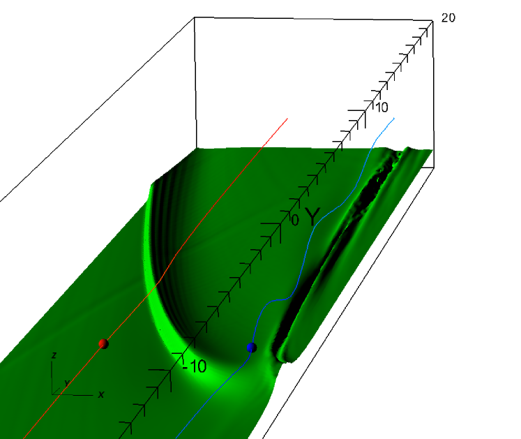
Figure 1.— The iso-density contour of $\rho=0.8\rho_{00}$ for an IA disk model. Planetary mass is increased to $M_{p}=0.3M_{th}$ to visually enhance the effect of buoyancy waves. Buoyancy waves cause ray-like density disturbances close to $x=0$ (right side of the box), which are also shown in Fig. 3. Two streamlines passing through (-0.5, 0, 1)(blue) and (-3, 0, 1)(red) demonstrate vertical oscillation due to buoyancy waves and the small velocity perturbation of sound waves.

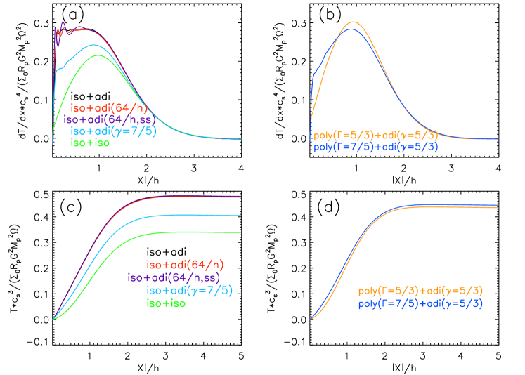
Figure 2.— Torque densities ($dT/dx$, upper panels) and integrated torques (lower panels) for disks with isothermal disk structure (left panels) and polytropic disk structure (right panels) with different EOS. Models II (green curves) and AA (orange curves) not supporting buoyancy waves exhibit a clear torque cut-off at $|x|\lesssim h$. All other models support buoyancy waves and show significant buoyancy torque near the planet.

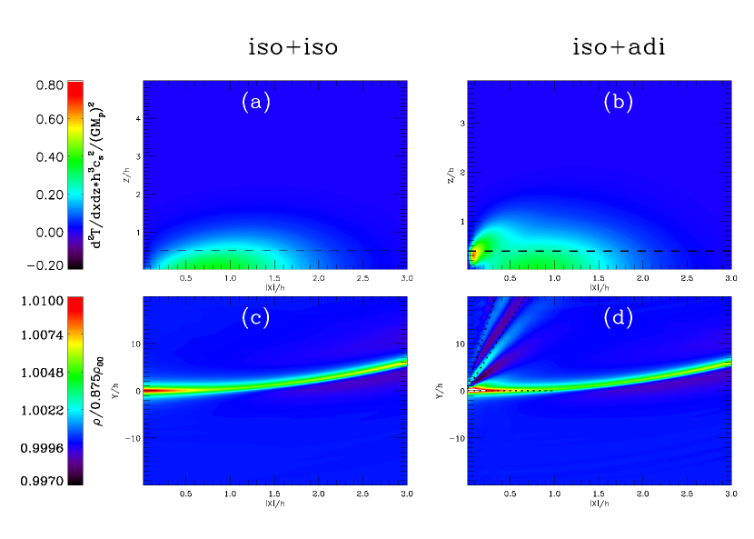
Figure 3.— Upper panels: (volume) density of the planet-induced torque integrated over $y$-coordinate for models II (left panel) and IA (right panel). Strong excess torque due to buoyancy waves close to the planet is clearly visible at $z\sim h$ in model IA, which features non-zero Brunt-Väisl̈ä frequency. Lower panels: density contours in the $xy$ plane at $z$ where $\rho_{0}$ equal to 0.8755 $\rho_{00}$ (indicated by the dashed line at $z\sim 0.5h$ in (a) and $z\sim 0.4h$ in (b), h are different in these two cases). Geometric locations corresponding to the resonance condition for buoyancy waves (11) are shown by dotted lines in model IA, and agree quite well with the pattern of density fluctuations derived from simulations.

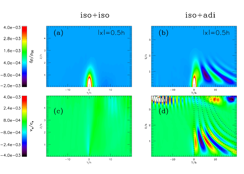
Figure 4.— Upper panels: density fluctuations in the $yz$ plane at $|x|=0.5h$ for models II (left panel) and IA (right panel). Lower panels: vertical velocity $v_{z}$ at $|x|=0.5h$ for models II and IA. The buoyancy resonance positions (11) are again plotted as dotted curves. The fluctuations of $v_{z}$ at $z>3h$ are due to the lack of exact hydrostatic equilibrium at the upper boundary.

References

- Artymowicz (1993) Artymowicz, P. 1993, ApJ, 419, 166
- Balmforth & Korycansky (2001) Balmforth, N. J., & Korycansky, D. G. 2001, MNRAS, 326, 833
- Baruteau & Masset (2008) Baruteau, C., & Masset, F. 2008, ApJ, 672, 1054
- Bate et al. (2002) Bate, M. R., Ogilvie, G. I., Lubow, S. H., & Pringle, J. E. 2002, MNRAS, 332, 575
- Bate et al. (2003) Bate, M. R., Lubow, S. H., Ogilvie, G. I., & Miller, K. A. 2003, MNRAS, 341, 213
- D’Angelo & Lubow (2010) D’Angelo, G., & Lubow, S. H. 2010, ApJ, 724, 730
- Dong et al. (2011) Dong, R., Rafikov, R. R., Stone, J. M., & Petrovich, C. 2011, ApJ, 741, 56
- Chiang & Goldreich (1997) Chiang, E. I., & Goldreich, P. 1997, ApJ, 490, 368
- Goodman & Rafikov (2001) Goodman, J., & Rafikov, R. R. 2001, ApJ, 552, 793
- Goldreich & Tremaine (1979) Goldreich, P., & Tremaine, S. 1979, ApJ, 233, 857
- Goldreich & Tremaine (1980) Goldreich, P., & Tremaine, S. 1980, ApJ, 241, 425
- Jang-Condell & Sasselov (2005) Jang-Condell, H., & Sasselov, D. D. 2005, ApJ, 619, 1123
- Kenyon & Hartmann (1987) Kenyon, S. J., & Hartmann, L. 1987, ApJ, 323, 714
- Korycansky & Pringle (1995) Korycansky, D. G., & Pringle, J. E. 1995, MNRAS, 272, 618
- Lin & Papaloizou (1993) Lin, D. N. C., & Papaloizou, J. C. B. 1993, Protostars and Planets III, 749
- Lin et al. (1990) Lin, D. N. C., Papaloizou, J. C. B., & Savonije, G. J. 1990, ApJ, 364, 326
- Lubow & Ogilvie (1998) Lubow, S. H., & Ogilvie, G. I. 1998, ApJ, 504, 983
- Lubow & Pringle (1993) Lubow, S. H., & Pringle, J. E. 1993, ApJ, 409, 360
- Lunine & Stevenson (1982) Lunine, J. I. & Stevenson, D. J. 1982, Icarus, 52, 14
- Masset (2001) Masset, F. S. 2001, ApJ, 558, 453
- Masset (2002) Masset, F. S. 2002, A&A, 387, 605
- Ogilvie & Lubow (2002) Ogilvie, G. I., & Lubow, S. H. 2002, MNRAS, 330, 950
- Paardekooper & Mellema (2006) Paardekooper, S.-J., & Mellema, G. 2006, A&A, 459, L17
- Paardekooper & Papaloizou (2008) Paardekooper, S.-J., & Papaloizou, J. C. B. 2008, A&A, 485, 877
- Rafikov (2002) Rafikov, R. R. 2002, ApJ, 572, 566
- Rafikov & Petrovich (2012) Rafikov, R. R. & Petrovich, C. 2012, ApJ, 747, 24
- Stone et al. (2008) Stone, J. M., Gardiner, T. A., Teuben, P., Hawley, J. F., & Simon, J. B. 2008, ApJS, 178, 137
- Stone & Gardiner (2010) Stone, J. M., & Gardiner, T. A. 2010, ApJS, 189, 142
- Takeuchi & Miyama (1998) Takeuchi, T., & Miyama, S. M. 1998, PASJ, 50, 141
- Tanaka et al. (2002) Tanaka, H., Takeuchi, T., & Ward, W. R. 2002, ApJ, 565, 1257
- Ward (1986) Ward, W. R. 1986, Icarus, 67, 164
- Ward (1997) Ward, W. R. 1997, Icarus, 126, 261