Parallel Semi-Implicit Time Integrators

Abstract

In this paper, we further develop a family of parallel time integrators known as Revisionist Integral Deferred Correction methods (RIDC) to allow for the semi-implicit solution of time dependent PDEs. Additionally, we show that our semi-implicit RIDC algorithm can harness the computational potential of multiple general purpose graphical processing units (GPUs) in a single node by utilizing existing CUBLAS libraries for matrix linear algebra routines in our implementation. In the numerical experiments, we show that our implementation computes a fourth order solution using four GPUs and four CPUs in approximately the same wall clock time as a first order solution computed using a single GPU and a single CPU.

I Introduction

RIDC methods are parallel–in–step time integrators [4, 6]. The “revisionist” terminology was first adopted in [4] to highlight that (i) this is a revision of the standard integral (or spectral) defect correction (IDC or SDC) methods [8, 7, 5, 9, 18, 22], and (ii) successive corrections, running in parallel but lagging in time, revise and improve the approximation to the solution. This notion of time parallelization is particularly exciting because it can be potentially layered upon existing spatial parallelization techniques [3, 26], including algorithms that utilize GPU cards to solve time dependent PDEs [16, 25, 1], to add further parallel scalability.

The main idea behind RIDC methods is to re-write the defect correction framework [27, 28] so that, after initial start-up costs, each correction loop can be lagged behind the previous correction loop in a manner that facilitates running the predictor and correctors in parallel. This idea for parallel time integrators was previously published by the present authors in [4, 6]. As before, this is still small scale parallelism in the sense that the time parallelization is limited by the order one wants to achieve.

To harness the computational potential of multiple graphical processing units (GPUs) on a single node, the CUBLAS library [23] (which is a collection of linear algebra subroutines coded in CUDA) are utilized to demonstrate that by threading the RIDC loops, multiple GPUs can be utilized for our semi-implicit RIDC algorithm. We present numerical experiments in Section IV to show that our algorithm and implementation computes a fourth order semi-implicit solution using four GPUs and four CPUs in approximately the same wall clock time as a first order forward-backward Euler solution computed using a single GPU and a single CPU. We stress that our parallel speedup comes from a unique way to utilize existing parallel libraries, in this case the CUBLAS libraries provided by NVIDIA. Unless data decomposition is used (whether in the host code or within a new parallel library), one could not use multiple GPU cards in as simple a fashion using a sequential ARK integrator. We believe that this work will provide the scientific community with a straightforward way to add further parallelism to existing software that generate low order (in time) solutions to time dependent PDEs using only a single GPU card.

Readers might be familiar with parareal integrators [13, 14, 19, 21, 15], another family of parallel time integrators. In such methods, the time domain is split into sub-problems that can be computed in parallel, and an iterative procedure for coupling the sub-problems is applied, so that the overall method converges to the solution of the full problem. Parareal integrators are philosophically different from RIDC methods. While parareal methods allow for large scale parallelization, there are non trivial choices of the fine and coarse predictor that affect convergence to the desired solution. RIDC methods on the other hand, guarantees convergence, and high order solutions. A class of parareal methods by Mike Minion and Matthew Emmett (CAMCOS, 2012) are potentially a generalization of the RIDC methods, but further analysis would be needed to validate that statement.

This paper is organized as follows: In Section II, we review Implicit–Explicit (IMEX) methods, which are a family of high order semi-implicit integrators [2, 17]. In Section III, semi-implicit RIDC methods and their properties are presented. Then, numerical benchmarks comparing RIDC and additive Runge–Kutta methods are given in Section IV, followed by concluding remarks in Section V.

II IMEX Methods

We are interested in solutions to initial value problems of the form,

$$\left\{\begin{array}[]{l}\displaystyle y^{\prime}(t)=f^{S}(t,y)+f^{N}(t,y),\quad t\in[a,b],\\ \displaystyle y(a)=\alpha.\end{array}\right.$$ (3)

where $y,\alpha\in\mathbb{R}^{n}$, $f^{N}:\mathbb{R}\times\mathbb{R}^{n}\to\mathbb{R}^{n}$ and $f^{S}:\mathbb{R}\times\mathbb{R}^{n}\to\mathbb{R}^{n}$. The function $f^{S}(t,y)$ contains stiff terms that need to be handled implicitly, and $f^{N}(t,y)$ consists of non-stiff terms that can be handled explicitly. A first order implicit-explicit (IMEX) discretization of the IVP (3) can be written as

$$\frac{y_{n+1}-y_{n}}{\Delta t}=f^{S}(t_{n+1},y_{n+1})+f^{N}(t_{n},y_{n}),\text{ with }y_{0}=\alpha.$$

The above IMEX discretization is particularly useful if $f^{S}(t,y)$ is linear in $y$, i.e. $f^{S}(t,y)=Dy$, which is often the case in a method of lines discretization of PDEs containing relaxation terms. In such cases, the IMEX discretization reduces to a linear system solve the solution at each time level,

$$(I-D\Delta t)y_{n+1}=y_{n}+\Delta tf^{N}(t_{n},y_{n}),\quad\text{with }y_{0}=\alpha.$$ (4)

An $s$-stage diagonally implicit RK (DIRK) and explicit $s$-stage explicit RK method are coupled

$$\begin{array}[]{c|cccc|ccccc}0&0&&&&0&&&&\\ c_{2}&a_{21}^{S}&a_{22}^{S}&0&\ldots&a_{21}^{N}&0&&&\\ \vdots&\vdots&\vdots&\ddots&&\vdots&&&\ddots&\\ c_{s}&a_{s1}^{S}&a_{s2}^{S}&\cdots&a_{ss}^{S}&a_{s1}^{N}&a_{s2}^{N}&\cdots&a_{s,s-1}^{N}&0\\ \hline\cr&b_{1}^{S}&b_{2}^{S}&\cdots&b_{s}^{S}&b_{1}^{N}&b_{2}^{N}&\cdots&b_{s-1}^{N}&b_{s}^{N}\end{array}$$

to generate a high order semi-implicit integrator. The discretization of IVP (3) using an IMEX method can be written as

$$y_{n+1}=y_{n}+\Delta t\sum_{i=1}^{s}\left(b_{i}^{S}K_{ni}^{S}+b_{i}^{N}K_{ni}^{N}\right),\quad\text{with }y_{0}=\alpha,$$

where the stages satisfy

$$K_{ni}^{S}=f^{S}(t_{ni},\,y_{n}+\Delta t\sum_{j=1}^{i}a_{ij}^{S}K_{nj}^{S}+\Delta t\sum_{j=1}^{i-1}a_{ij}^{N}K_{nj}^{N})$$

$$K_{ni}^{N}=f^{N}(t_{ni},\,y_{n}+\Delta t\sum_{j=1}^{i}a_{ij}^{S}K_{nj}^{S}+\Delta t\sum_{j=1}^{i-1}a_{ij}^{N}K_{nj}^{N}).$$

with $t_{ni}=t+c_{i}\Delta t$. The third and fourth order IMEX methods from [20] are used to benchmark against our fourth order RIDC-FBE (RIDC constructed using forward and backward Euler integrators). The third order IMEX method is constructed from the following Butcher tableaux:

$$\begin{array}[]{c|rrrrr|rrrrr}0&0&&&&&0&&&&\\ \frac{1}{2}&0&\frac{1}{2}&&&&\frac{1}{2}&&&&\\ \frac{1}{2}&\frac{1}{4}&-\frac{5}{12}&\frac{2}{3}&&&\frac{1}{4}&\frac{1}{4}&&&\\ 1&2&-\frac{7}{2}&\frac{1}{2}&2&&0&1&0&&\\ 1&\frac{1}{6}&0&\frac{2}{3}&-\frac{5}{6}&1&\frac{1}{6}&0&\frac{2}{3}&\frac{1}{6}&\\ \hline\cr&\frac{1}{6}&0&\frac{2}{3}&-\frac{5}{6}&1&\frac{1}{6}&0&\frac{2}{3}&\frac{1}{6}&\end{array}$$

The fourth order IMEX method is constructed from the following DIRK method

$$\begin{array}[]{c|rrrrrrr}0&0&&&&&&\\ \frac{1}{3}&-\frac{1}{6}&\frac{1}{2}&&&&&\\ \frac{1}{3}&\frac{1}{6}&-\frac{1}{3}&\frac{1}{2}&&&&\\ \frac{1}{2}&\frac{3}{8}&-\frac{3}{8}&0&\frac{1}{2}&&&\\ \frac{1}{2}&\frac{1}{8}&0&\frac{3}{8}&-\frac{1}{2}&\frac{1}{2}&&\\ 1&-\frac{1}{2}&0&3&-3&1&\frac{1}{2}&\\ 1&\frac{1}{6}&0&0&0&\frac{2}{3}&-\frac{1}{2}&\frac{2}{3}\\ \hline\cr&\frac{1}{6}&0&0&0&\frac{2}{3}&-\frac{1}{2}&\frac{2}{3}\end{array}$$

and explicit RK method

$$\begin{array}[]{c|rrrrrrr}0&0&&&&&&\\ \frac{1}{3}&\frac{1}{3}&&&&&&\\ \frac{1}{3}&\frac{1}{6}&\frac{1}{6}&&&&&\\ \frac{1}{2}&\frac{1}{8}&0&\frac{3}{8}&&&&\\ \frac{1}{2}&\frac{1}{8}&0&\frac{3}{8}&0&&&\\ 1&\frac{1}{2}&0&-\frac{3}{2}&0&2&&\\ 1&\frac{1}{6}&0&0&0&\frac{2}{3}&\frac{1}{6}&\\ \hline\cr&\frac{1}{6}&0&0&0&\frac{2}{3}&\frac{1}{6}&0\end{array}$$

(Note, a second order IMEX scheme was also tested, but not presented because of its poor stability constraints). Similar to before, if $f^{S}(t,y)$ is linear in $y$, then each stage computation reduces to a linear solve since a DIRK method was paired with an explicit integrator in the discussed IMEX methods.

III RIDC Methods

RIDC methods are a class of time integrators based on integral deferred correction [10]. RIDC methods first compute a prediction to the solution (“level 0”) using low order schemes (e.g. a first order implicit-explicit method) followed by one or more corrections to compute subsequent solution levels. Each correction revises the solution and increases the formal order of accuracy by $1$, if a first order implicit-explicit integrator is used to solve the error equation. Each correction level is delayed from the previous level as illustrated in Figure 1 – the open circles denote solution values that are simultaneously computed. This staggering in time means that the predictor and each corrector can all be executed simultaneously, in parallel, while each processes a different time-step.

Figure 1: (RIDC4-FBE) This plot shows the staggering required for a fourth order RIDC scheme, constructed using a first order implicit–explicit predictors and correctors. The time axis runs horizontally, and the correction levels run vertically. The white circles denote solution values that are simultaneously computed, e.g., core 0 is computing the prediction solution at time $t_{n+2}$ while core 1 is computing the 1st corrected solution at time $t_{n+1}$, etc.

In Section III-A, we first derive the error equation. Then, Section III-B and Section III-C give numerical schemes for solving the IVP and the error equation. In Section III-D, we review theorems related to the formal order of accuracy that follow trivially from [5], and in Section III-E, we summarize starting and stopping details for the RIDC algorithm as well as the notion of restarts.

III-A Error Equation

Suppose an approximate solution $\eta(t)$ to IVP (3) is computed. Denote the exact solution as $y(t)$. Then, the error of the approximate solution is

$$e(t)=y(t)-\eta(t).$$ (5)

If we define the residual as $\epsilon(t)=\eta^{\prime}(t)-f^{S}(t,\eta(t))-f^{N}(t,\eta(t))$, then the derivative of the error (5) satisfies

$$e^{\prime}(t) =y^{\prime}(t)-\eta^{\prime}(t)$$

$$=f^{S}(t,y(t))+f^{N}(t,y(t))-f^{S}(t,\eta(t))$$

$$\phantom{=}-f^{N}(t,\eta(t))-\epsilon(t).$$

The integral form of the error equation,

$$\left[e(t)+\int_{a}^{t}\epsilon(\tau)\,d\tau\right]^{\prime}=f^{S}\left(t,\eta(t)+e(t)\right)-f^{S}\left(t,\eta(t)\right)$$

$$+f^{N}\left(t,\eta(t)+e(t)\right)-f^{N}\left(t,\eta(t)\right),$$ (6)

can then be solved using the initial condition $e(a)=0$.

III-B The predictor

To generate a provisional solution that can be corrected, a low order integrator is applied to solve IVP (3); this process is typically known as the prediction loop. The first-order IMEX scheme reviewed in Section II will be used to generate our RIDC-FBE (RIDC forward and backward Euler method) though in theory, any IMEX methods reviewed in Section II can be used. We adopt the following notation:

$$\eta^{[0]}_{n+1}=\eta^{[0]}_{n}+\Delta t_{n}f^{S}(t_{n+1},\eta^{[0]}_{n+1})+\Delta t_{n}f^{N}(t_{n},\eta^{[0]}_{n}),$$ (7)

where the superscript ^[0] indicates this is the solution at level $0$, the prediction level. This non-linear equation can be solved using Newton’s method.

III-C The corrector

The correctors are also low order integrators, but are used to solve the error equation (6) for the error $e(t)$ to an approximate solution $\eta(t)$. Since the error equation is solved iteratively to improve a solution from the previous level, each correction level computes an error $e^{[j-1]}(t)$ to the solution at the previous level $\eta^{[j-1]}(t)$ to obtain a revised solution $\eta^{[j]}(t)=\eta^{[j-1]}(t)+e^{[j-1]}(t)$.

A first order IMEX discretization of the error equation (6) (after some algebra) gives

$$\eta^{[j]}_{n+1}=\eta^{[j]}_{n}+\Delta t\left[f^{S}(t_{n+1},\eta^{[j]}_{n+1})+f^{N}(t_{n},\eta^{[j]}_{n})\right]$$ (8)

$$-\left[\Delta tf^{S}(t_{n+1},\eta^{[j-1]}_{n+1})+f^{N}(t_{n},\eta^{[j-1]}_{n})\right]$$

$$+\int_{t_{n}}^{t_{n+1}}f(\tau,\eta^{[j-1]}(\tau))\,d\tau.$$

The integral $\int_{t_{n}}^{t_{n+1}}f(\tau,\eta^{[j-1]}(\tau))\,d\tau$ is approximated using quadrature. For the $j$^th correction loop, $(j+1)$ nodes are needed in the stencil to accurately approximate the integral. There are various choices for the stencil, but in practice, the stencil should include the nodes $t_{n}$ and $t_{n+1}$. We make the following choice for selecting our quadrature nodes:

$$\int_{t_{n}}^{t_{n+1}}f(\tau,\eta^{[j-1]}(\tau))\,d\tau\approx$$ (9)

$$\begin{cases}\sum_{k=0}^{j}\alpha_{nk}\left(f^{N}(t_{n+1-k},\eta^{[j-1]}_{n+1-k})+f^{S}(t_{n+1-k},\eta^{[j-1]}_{n+1-k})\right),\\ \hskip 180.67499pt\mbox{if }(n\geq j-1)\\ \sum_{k=0}^{j}\alpha_{nk}\left(f^{N}(t_{k},\eta^{[j-1]}_{k})+f^{S}(t_{k},\eta^{[j-1]}_{k})\right),\\ \hskip 180.67499pt\mbox{if }(n<j-1)\end{cases}$$

where the quadrature weights are given by

$$\alpha_{nk}=\int_{t_{n}}^{t_{n+1}}\prod_{i=0,i\neq k}^{j}\frac{(t-t_{n+1-i})}{(t_{n+1-k}-t_{n+1-i})}\,dt,$$

for $n\geq j-1$, $k=0,1,\ldots,j-1$, and

$$\alpha_{nk}=\int_{t_{n}}^{t_{n+1}}\prod_{i=0,i\neq k}^{j}\frac{(t-t_{i})}{(t_{k}-t_{i})}\,dt,\quad k=0,1,\ldots,j-1$$

for $n<j-1$. Since uniform time steps are used in the computation, then only one set of quadrature weights needs to be computed, stored, then used as necessary.

III-D Formal order of accuracy

The analysis in [5], proving convergence under mild conditions for IDC-IMEX methods, extends simply to these RIDC-IMEX methods.

Theorem III.1.

Let $f(t,y)$ and $y(t)$ in IVP (3) be sufficiently smooth. Then, the local truncation error for a RIDC method constructed using a first order IMEX integrators for the predictor and $(p-1)$ correction loops is $\mathcal{O}(\Delta t^{p+1})$.

Theorem III.2.

Let $f(t,y)$ and $y(t)$ in IVP (3) be sufficiently smooth. Then, the local truncation error for an RIDC method constructed using uniform time steps, a $p_{0}$^th-order ARK method in the prediction loop, and $(p_{1},p_{2},\cdots,p_{j})$^th-order ARK methods in the correction loops, is $\mathcal{O}(\Delta t^{p+1})$, where $p=\sum_{i=0}^{j}p_{i}$.

III-E Further Comments

During most of a RIDC calculation, multiple solution levels are marched in a pipe using multiple computing CPUs/GPUs. However, the computing nodes in the RIDC algorithm cannot start simultaneously: each must wait for the previous level to compute sufficient $\eta$ values before they can be marched in a pipeline fashion. By carefully controlling the start-up of a RIDC method, one can minimize the amount of memory that is required to march the nodes in a pipeline fashion. In our implementation, the order in which computations are performed during start-up is illustrated in Figure 2 for a fourth order RIDC constructed with first order IMEX predictors and correctors. The $j$^th processor (running the $j\textsuperscript{th}$ correction) must initially wait for $j(j+1)/2$ steps, e.g., node 2 has to wait 3 steps before starting.

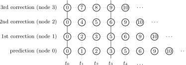
Figure 2: This figure is a graphical representation of how the RIDC4-BE algorithm is started. The time axis runs horizontally, the correction levels run vertically. All nodes are initially populated with the initial data at $t_{0}$. This is represented by computing step 0 (enclosed in a circle). At computing step 1, node 0 computes the predicted solution at $t_{1}$. The remaining nodes remain idle. At computing step 2, node 0 computes the predicted solution at time $t_{2}$, node 1 computes the 1st corrected solution at time $t_{1}$, the remaining two nodes remain idle. Note that in this starting algorithm, special care is taken to ensure that minimum memory is used by not letting the computing cores run ahead until they can be marched in a pipeline; in this example, when node 3 starts computing $t_{3}$.

There are also idle computing threads at the end of the computation, since the predictor and lower level correctors will reach $t_{N}=b$ earlier than the last corrector.

An important notion to consider is “restarts”, that is, instead of computing all the way to the final time, we compute on some smaller time interval to time $t_{\star}$, and use the most accurate solution to restart the RIDC computation at $t=t_{\star}$. In practice, restarting improves the stability of the semi implicit RIDC scheme, and could lower the error constant of the overall method, but at the cost of decreasing the speedup due to the additional cost of starting the RIDC algorithm multiple times.

Additionally, one cannot increase the order of RIDC indefinitely as (i) it is not practical (when would one ever want a 16th order method?) and (ii) the Runge phenomenon [24], which arises from using equi-spaced interpolation points, will eventually cause the scheme to become unstable. In practice, 8th and 12th order RIDC methods using double precision do not suffer from the Runge phenomenon.

Lastly, there is another family of parallel time integrators, known as parareal methods [21], that is actively being researched [11, 12]. These methods fall into the class of “parallel across the method” algorithms, where the entire time domain is split across multiple nodes, a coarse operator is run in serial, followed by a parallel correction update. We encourage users to more carefully consider parareal if the small scale parallelism offered by RIDC is not sufficient.

IV Numerical Examples

Advection–reaction–diffusion equations have been widely used to model chemical processes across many disciplines. Here, we present two numerical examples: an advection–diffusion and a reaction–diffusion equation, to validate the order of accuracy of the RIDC4-FBE scheme, and the speedup obtained in the parallel OpenMP framework, and the OpenMP–CUDA hybrid framework. In each example, the stiff term is chosen as the diffusion operator, $f^{S}(t,y)=y_{xx}$. Applying a centered finite difference operator to approximate $\partial_{xx}$ reduces each RIDC/ARK step to a series of decoupled linear system solves. The matrices are pre-factored into their QR components so that each linear solve is reduced to a matrix–vector multiplication and a back solve operation.

The computations presented were performed on a stand alone server containing a quad core AMD Phenom X4 9950 2.6Ghz processor with four Nvidia Tesla GPU C1060 cards (960 total GPU cores). (Superior speedups will be observed with the newer Nvidia Tesla M2090 cards that are rated at 665 Gflops at double precision, compared with the legacy M1060 cards that are rated at 78 Gflops at double precision.) The ARK schemes are coded using plain C++ with (i) a homegrown linear algebra library and (ii) the CUBLAS 4.0 library [23]. The RIDC4-FBE is coded in C++ with (i) OpenMP and the homegrown linear algebra library, and (ii) OpenMP and the CUBLAS 4.0 library. Some important subtleties for creating a hybrid OpenMP – CUDA RIDC code are: (i) we can control which GPU card is used for a linear solve by calling the cudaSetDevice() function, and (ii) in using “#pragma for” loop to spawn individual threads for each prediction/correction loop, we have to utilize static scheduling.

We note that to illustrate the effectiveness of parallel time integrators in our numerical examples, we chose 1D problems so that by taking a fine spatial resolution, the temporal discretization error would dominate the spatial error. Solutions to higher dimensional solutions are practical with the newer available Fermi/Keppler cards which have more onboard memory.

IV-A Advection-Diffusion

We first consider the canonical advection-diffusion problem to show that we can achieve designed orders of accuracy for our RIDC-FBE algorithm. The constant coefficient advection-diffusion equation,

$$u_{t}=cu_{x}+du_{xx},\quad x\in[0,1],\quad t\in[0,40],$$

$$u(x,0)=2+\sin(2\pi x),$$

with periodic boundary conditions, is discretized using the method of lines methodology. Specifically, the advection term is discretized using upwind first order differences, and the diffusion term is discretized using central differences. The following system is then recovered:

$$u_{t}=Au+Du,\quad u(0)=\alpha,$$

where the matrix $A$ approximates the advection operator, and the matrix $D$ approximates the diffusion operator. We choose the obvious splitting, $f^{N}(t,u)=Au$, and $f^{S}(t,u)=Du$. We take $c=0.1,d=10^{-3},\Delta x=\frac{1}{1000}$. First, we show in Figure 3a that ARK and RIDC4 achieve their designed orders of accuracy. Observe that the error coefficient for ARK4 is several orders of magnitude smaller than that of RIDC4. In Figure 3b, we instead plot the results from the same numerical run, this time plotting error as a function of the wall clock time. Several observations can be made: (i) for all the schemes, our GPU implementation is approximately an order of magnitude faster than the CPU implementation, (ii) RIDC4 (both the CPU and GPU implementations) compute a fourth order solution in the same wall clock as the FBE solution, (iii) for a fixed wall clock time, RIDC4 (with 4 GPUs) computes a solution that is several orders of magnitude more accurate than the solution computed using ARK4 (with 1 GPU).

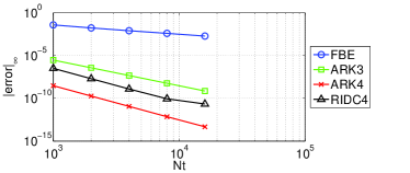
(a) Convergence study: error versus number of time steps

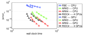
(b) error versus wall clock time

Figure 3: (a) This standard “error versus step size” convergence study for RIDC4-FBE (with 10 restarts) and the various ARK methods presented in section II. All schemes achieve their designed orders of accuracy. Observe that the RIDC4-FBE error coefficient is much larger than that of the ARK4 scheme. This is a small price to pay for the parallel speedup that can be obtained, as shown in (b). Two observations should be made: (i) for all the schemes, our GPU implementation is approximately an order of magnitude faster than the CPU implementation, (ii) RIDC4 (both the CPU and GPU implementations) compute a fourth order solution in the same wall clock as the FBE solution.

We also show in Figure 4 the error of RIDC4 as a function of restarts. As expected, the error decreases as the number of restarts is increased. The penalty for each restart is having to fill the memory footprint at each restart before marching the cores/GPUs in a pipe.

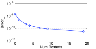
Figure 4: The error of RIDC4 schemes at the final time $T=40$ decreases as the number of restarts is increased (for a fixed number of time steps, in this case, 4000 time steps). Each restart requires that the memory footprint be refilled before the cores/GPUs can be marched in a pipe.

Table I summarizes the speedup that is obtained when RIDC4 is computed using one, two and four CPUs, and when RIDC4 is computed using one, two and four GPUs. We appear to obtain almost linear speedup, even with 10 restarts. This scaling is not surprising since a bulk of the computational cost is due to the linear solve and data transfer between host and GPU memory is not limited by bandwidth for our example.

# CPUs	Speedup
1	1.0
2	1.89
4	3.81

# CPUs & GPUs	Speedup
1	1.0
2	1.97
4	3.88

TABLE I: Speedup of RIDC for the advection–diffusion problem.

The percentage of time that GPUs spend calling CUBLAS kernels are summarized in the Table II. As the table indicates, data transfer is a minimal component of our CUDA code.

kernel	calls	% GPU time
trsv_kernel	5061	73.3%
gemv2N_kernel_ref	11181	20.47%
gemv2T_kernel_ref	5061	3.98%
axpy_kernel_ref	24200	1.15%
memcpyHtoD	8243	0.61%
memcpyDtoH	5061	0.43%

TABLE II: Profiling our GPU code for the advection–diffusion problem.

IV-B Viscous Burgers’ Equation

We also consider the solution to viscous Burgers’ equation,

$$u_{t}+\frac{1}{2}\left(u^{2}\right)_{x}=\epsilon u_{xx},\quad(x,t)\in[0,1]\times[0,1],$$

with initial and boundary conditions

$$u(0,t)=u(1,t)=0,\quad u(x,0)=\sin{(2\pi x)}+\frac{1}{2}\sin{(\pi x)}.$$

The solution develops a layer that propagates to the right, as shown in Figure 5.

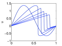
Figure 5: Solution to Burgers’ equation, with $\epsilon=10^{-3}$ and $\Delta x=\frac{1}{1000}$. Time snapshots at $t=0,0.2,0.4,0.6,0.8$ and $1$ are shown.

The diffusion term is again discretized using centered finite differences. A numerical flux is used to approximate the advection operator,

$$\frac{1}{2}((u_{i}^{n})^{2})_{x}=\frac{1}{2}\frac{f^{n}_{i+1/2}-f^{n}_{i-1/2}}{\Delta x},$$

where

$$f_{i+1/2}^{n}=\frac{1}{2}\left((u_{i+1}^{n})^{2}+(u_{i}^{n})^{2}\right).$$

Hence, the following system of equations is obtained,

$$u_{t}=\mathcal{L}(u)+Du,$$

where the operator $\mathcal{L}(u)$ approximates the hyperbolic term using the numerical flux, and the matrix $D$ approximates the diffusion operator. We choose the splitting $f^{N}(t,u)=\mathcal{L}(u)$ and $f^{S}(t,u)=Du$, and take $\epsilon=10^{-3}$ and $\Delta x=\frac{1}{1000}$. No restarts are used for this simulation.

The same numerical results as the previous advection–diffusion example are observed in Figure 6. In plot (a), the RIDC scheme achieves it’s designed order of accuracy. In plot (b), we show that our RIDC implementations (both the CPU and GPU versions) obtain a fourth order solution in the same wall clock time as a first order semi-implicit FBE solution. The RIDC implementations with multiple CPU/GPU resources also achieve comparable errors to a fourth order ARK scheme in approximately one tenth the time.

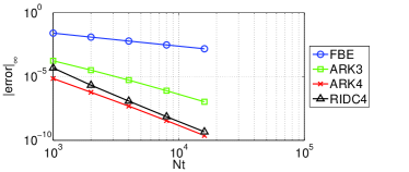
(a) Convergence study: error versus number of time steps

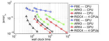
(b) error versus wall clock time

Figure 6: In (a), we show that the ARK schemes and our RIDC4-FBE scheme achieve the designed orders of accuracy. The plot in (b) shows the error as a function of wall clock time. Two observations should be made: (i) for all the schemes, our GPU implementation is approximately an order of magnitude faster than the CPU implementation.

Table III summarizes the speedup that is obtained when RIDC4 is computed using one, two and four CPUs, and when RIDC4 is computed using one, two and four GPUs.

# CPUs	Speedup
1	1.0
2	1.94
4	3.94

# CPUs & GPUs	Speedup
1	1.0
2	1.98
4	3.95

TABLE III: Speedup of RIDC for Burgers’ equation.

V Conclusions

In this paper, we further developed RIDC algorithms to generate a family of high order semi-implicit parallel integrators. The analysis related to convergence is a simple extension from previous work, and the numerical experiments demonstrate that the fourth order RIDC-FBE algorithm achieves its designed order of accuracy. Additionally, we showed that our semi-implicit RIDC algorithm harnessed the computational potential of four GPUs by utilizing OpenMP coupled with with the CUBLAS library. This semi-implicit RIDC algorithm can potentially be coupled with existing legacy parallel spatial codes. Work is on-going to explore a hybrid MPI–OpenMP–CUDA algorithm for more heterogeneous architectures.

References

- [1] Joshua A. Anderson, Chris D. Lorenz, and A. Travesset. General purpose molecular dynamics simulations fully implemented on graphics processing units. Journal of Computational Physics, 227(10):5342 – 5359, 2008.
- [2] Uri M. Ascher, Steven J. Ruuth, and Brian T. R. Wetton. Implicit-explicit methods for time-dependent partial differential equations. SIAM J. Numer. Anal., 32(3):797–823, 1995.
- [3] Andrew Christlieb, Ron Haynes, and Benjamin Ong. A parallel space–time algorithm. submitted.
- [4] Andrew Christlieb, Colin Macdonald, and Benjamin Ong. Parallel high-order integrators. SIAM J. Sci. Comput., 32(2):818–835, 2010.
- [5] Andrew Christlieb, Maureen Morton, Benjamin Ong, and Jing-Mei Qiu. Semi-implicit integral deferred correction constructed with high order additive Runge-Kutta integrators. Comm. Math. Sci, 9(3):879–902, 2011.
- [6] Andrew Christlieb and Benjamin Ong. Implicit parallel time integrators. J. Sci. Comput., 49(2):167–179, 2011.
- [7] Andrew Christlieb, Benjamin Ong, and Jing-Mei Qiu. Comments on high order integrators embedded within integral deferred correction methods. Comm. Appl. Math. Comput. Sci., 4(1):27–56, 2009.
- [8] Andrew Christlieb, Benjamin Ong, and Jing-Mei Qiu. Integral deferred correction methods constructed with high order Runge-Kutta integrators. Math. Comput., 79:761–783, 2010.
- [9] Alok Dutt, Leslie Greengard, and Vladimir Rokhlin. Spectral deferred correction methods for ordinary differential equations. BIT, 40(2):241–266, 2000.
- [10] Alok Dutt, Leslie Greengard, and Vladimir Rokhlin. Spectral deferred correction methods for ordinary differential equations. BIT, 40(2):241–266, 2000.
- [11] W. Elwasif, S. Foley, D. Bernholdt, L. Berry, D. Samaddar, Newman D., and R Sanchez. A dependency-driven formulation of parareal: Parallel-in-time solution of pdes as a many-task application. 4th IEEE Workshop on Many-Task Computing on Grids and Supercomputers, submitted.
- [12] M. Emmett and M. Minion. Towards an efficient parallel in time method for partial differential equations. Journal of Computational Physics, submitted.
- [13] M.J. Gander and E. Hairer. Nonlinear convergence analysis for the parareal algorithm. Lecture Notes in Computational Science and Engineering, 60:45, 2008.
- [14] M.J. Gander and S. Vandewalle. Analysis of the parareal time-parallel time-integration method. SIAM J. Sci. Comput., 29(2):556–578, 2007.
- [15] M.J. Gander and S. Vandewalle. On the superlinear and linear convergence of the parareal algorithm. Lecture Notes in Computational Science and Engineering, 55:291, 2007.
- [16] Christian Janßen and Manfred Krafczyk. Free surface flow simulations on gpgpus using the lbm. Computers and Mathematics with Applications, 61(12):3549 – 3563, 2011.
- [17] Christopher A. Kennedy and Mark H. Carpenter. Additive Runge–Kutta schemes for convection-diffusion-reaction equations. Appl. Numer. Math., 44(1-2):139–181, 2003.
- [18] Anita T. Layton and Michael L. Minion. Implications of the choice of predictors for semi-implicit Picard integral deferred correction methods. Commun. Appl. Math. Comput. Sci., 2:1–34 (electronic), 2007.
- [19] J.L. Lions, Y. Maday, and G. Turinici. A “parareal” in time discretization of PDEs. Comptes Rendus de l’Academie des Sciences Series I Mathematics, 332(7):661–668, 2001.
- [20] Hongyu Liu and Jun Zou. Some new additive Runge–Kutta methods and their applications. J. Comput. Appl. Math., 190(1-2):74–98, 2006.
- [21] Y. Maday and G. Turinici. A parareal in time procedure for the control of partial differential equations. Comptes rendus-Mathématique, 335(4):387–392, 2002.
- [22] Michael L. Minion. Semi-implicit spectral deferred correction methods for ordinary differential equations. Commun. Math. Sci., 1(3):471–500, 2003.
- [23] Nvidia. NVIDIA CUDA C programming guide, 2011. http://developer.nvidia.com.
- [24] Carl Runge. Über empirische Funktionen und die Interpolation zwischen äquidistanten Ordinaten. Zeit. für Math. und Phys., 46:224–243, 1901.
- [25] Daisuke Sato, Yuanfang Xie, James Weiss, Zhilin Qu, Alan Garfinkel, and Allen Sanderson. Acceleration of cardiac tissue simulation with graphic processing units. Medical and Biological Engineering and Computing, 47:1011–1015, 2009. 10.1007/s11517-009-0514-4.
- [26] Andrea Toselli and Olof Widlund. Domain decomposition methods—algorithms and theory, volume 34 of Springer Series in Computational Mathematics. Springer-Verlag, Berlin, 2005.
- [27] P. E. Zadunaisky and G. Lafferriere. On an iterative improvement of the approximate solution of some ordinary differential equations. Comput. Math. Appl., 6(1, Special Issue):147–154, 1980.
- [28] Pedro E. Zadunaisky. On the estimation of errors propagated in the numerical integration of ordinary differential equations. Numer. Math., 27(1):21–39, 1976/77.