The Green Bank Telescope $\mathbf{350\;\textrm{MHz}}$ Drift-scan Survey II: Data Analysis and the Timing of 10 New Pulsars, Including a Relativistic Binary

Abstract

We have completed a $350\;\textrm{MHz}$ drift scan survey using the Robert C. Byrd Green Bank Telescope with the goal of finding new radio pulsars, especially millisecond pulsars that can be timed to high precision. This survey covered $\sim$10300 square degrees and all of the data have now been fully processed. We have discovered a total of 31 new pulsars, seven of which are recycled pulsars. A companion paper by Boyles et al. (2012) describes the survey strategy, sky coverage, and instrumental set-up, and presents timing solutions for the first 13 pulsars. Here we describe the data analysis pipeline, survey sensitivity, and follow-up observations of new pulsars, and present timing solutions for 10 other pulsars. We highlight several sources—two interesting nulling pulsars, an isolated millisecond pulsar with a measurement of proper motion, and a partially recycled pulsar, PSR J0348+0432, which has a white dwarf companion in a relativistic orbit. PSR J0348+0432 will enable unprecedented tests of theories of gravity.

1 Introduction

The vast majority of observed neutron stars in the Galaxy manifest themselves as radio pulsars. The extremely high rotational stability of pulsars, and especially millisecond pulsars (MSPs), make them unrivaled laboratories for studying a wide range of astrophysical phenomena. Most pulsars have been discovered in large-area surveys, but most of these have focused on southern declinations or narrow regions around the Galactic plane. There is a need to find more pulsars in the northern sky, particularly high-precision MSPs that can be included in a pulsar timing array to detect gravitational waves (e.g. Jenet et al., 2009). The $100$-m Robert C. Byrd Green Bank Telescope (GBT) is one of the best telescopes in the world for finding and studying pulsars and a visible-sky pulsar survey using the GBT is underway (the Green Bank North Celestial Cap survey).

During the northern summer of 2007 the azimuth track of the GBT underwent repair, making normal operations impossible. Our team took advantage of the situation by completing the GBT $350\;\textrm{MHz}$ Drift-scan Survey between May and August. Because the GBT was unable to move in azimuth, we observed at a number of fixed elevations and allowed the sky to drift through the telescope beam at the sidereal rate. This survey was one of several low-frequency GBT surveys that are optimized for finding bright, nearby pulsars, with an emphasis on MSPs. These surveys have either been completed (Hessels et al., 2008), are ongoing, or are planned for the future. We collected over 1491 hours of data totaling $134\;\mathrm{TB}$. Approximately $30\;\mathrm{TB}$ of these data are being analyzed by the Pulsar Search Collaboratory, an educational initiative that actively involves high school students and teachers in research under the guidance of a team of astronomers (Rosen et al., 2010). For the remainder of this paper we discuss only the $\sim$$100\;\mathrm{TB}$ of the data that we have analyzed ourselves. All of these data have been fully processed and we have discovered 31 new pulsars, including ten recycled pulsars (seven of which are MSPs with $P<10\;\textrm{ms}$). We have derived full timing solutions for 25 of these new pulsars. The first 13 pulsars are being presented in a companion paper (Boyles et al., 2012, hereafter Paper I), along with a detailed description of the survey strategy, sky coverage, and instrumental set-up. We present timing solutions for an additional 10 pulsars here and describe the survey pipeline and data analysis in detail. An earlier-discovered Drift-scan pulsar, PSR J1023$+$0038, has been discussed elsewhere (see Archibald et al., 2009, 2010), while another MSP, PSR J2256$-$1024, will be presented in a future paper (Stairs et al. in prep). In §2 we explain how the data were divided into regions on the sky, interference removal, our de-dispersion scheme, and search strategies. In §3 we describe our approximate survey sensitivity and the effects of scattering. In §4 we describe how we confirmed candidate pulsars and our follow-up observations. In §5 we present timing solutions and discuss some interesting individual systems. A summary can be found in §6.

2 Data Analysis

The Drift-scan survey covered $\sim$10300 square degrees. A detailed description of the survey strategy, sky coverage, and instrumental set-up can be found in Paper I. Here we focus on the data reduction and search techniques. All data were processed using the PRESTO software suite (Ransom, 2001).

2.1 Pseudo-Pointings and Interference Excision

Data were collected while the azimuth track of the GBT was being repaired, so the telescope was locked at constant azimuth. Different regions of the sky were observed by changing the elevation of the telescope and allowing the sky to drift through the telescope beam at the sidereal rate. The time for a given point on the sky to pass through the beam is

$$t\simeq\frac{b}{\mathcal{R}_{\mathrm{sid}}\cos{\delta}},$$ (1)

where $b=36^{\prime}$ is the full-width-at-half-maximum of the GBT beam at $350\;\textrm{MHz}$, $\mathcal{R}_{\mathrm{sid}}=15^{\prime}\,\min^{-1}$ is the sidereal rate, and $\delta$ is the declination. The survey covered $-8^{\circ}\lesssim\delta\lesssim+38^{\circ}$ and $-21^{\circ}\lesssim\delta\lesssim+38^{\circ}$, depending on the azimuth of the telescope (see Paper I for details). Although the telescope was not actually tracking the sky, we defined an individual pseudo-pointing to be a continuous block of data $\sim$$140\;\textrm{s}$ in duration. Each pseudo-pointing overlapped with the preceding one by $70\;\textrm{s}$, so that all of our data were processed as part of two different pseudo-pointings.

The raw data were collected using the GBT Pulsar Spigot back-end (Kaplan et al., 2005). The Spigot uses autocorrelation chips that each work on 3-level raw samples and create an adjustable number of lags. These are then integrated into either 8- or 16-bit values, depending on the mode. The center frequency of the observations was $350\;\textrm{MHz}$ and the bandwidth was $50\;\textrm{MHz}$. Most of our observations were made using the 8-bit mode that split the band into 2048 lags which were fast Fourier transformed to synthesize 2048 frequency channels, each with a width of $24.4\;\textrm{kHz}$, and recorded every $81.92\;\mathrm{\mu s}$. A relatively small amount of data was taken early in the survey using the 16-bit, 1024 channel mode with the same sampling time. Hence, each $140\;\textrm{s}$ block of data consisted of roughly 1.7 million spectra.

Each pseudo-pointing was independently analyzed for radio frequency interference (RFI) using the rfifind tool from PRESTO. Data were broken into blocks roughly two seconds long while maintaining the full frequency resolution. The total power, mean, and variance in both the time and frequency domain were calculated for each data block and compared to the median quantity for the entire pseudo-pointing. A time/frequency block was flagged as RFI and masked out (i.e. set to zero) in future analysis if the value of total power, mean power, or variance was greater than ten/four standard deviations from the median values for the entire pseudo-pointing. If greater than 30%/70% of time intervals/channels were flagged then all remaining intervals/channels were masked out as well, under the assumption that they probably contained RFI just below our cut-off threshold. In addition to blindly searching for RFI, the Fourier spectra were de-reddened and persistent, well known sources of interference (e.g. the $60\;\textrm{Hz}$ signal from AC power sources) were explicitly removed from the power spectra of each pseudo-pointing. Despite the fact that there was significant construction on-site due to the track repair, our data were remarkably free of RFI. For example, the median masking fraction was 0.56% and only 0.2% of the data had a masking fraction greater than 30%. We are confident that we reached the noise limit for the vast majority of our survey (see §3).

2.2 De-Dispersion

Free electrons in the interstellar medium give rise to a frequency-dependent dispersive time delay which, if left uncorrected, will make it virtually impossible to find new pulsars. The magnitude of the delay between two frequencies, $\nu_{1}$ and $\nu_{2}$, is

$$t_{\mathrm{DM}}\simeq 4.15\times 10^{3}\;\textrm{s}\times\textrm{DM}\times\left[\left(\frac{\nu_{1}}{\textrm{MHz}}\right)^{-2}-\left(\frac{\nu_{2}}{\textrm{MHz}}\right)^{-2}\right],$$ (2)

where DM is the dispersion measure in units of $\mathrm{pc\;cm^{-3}}$. After applying appropriate shifts to each frequency channel, we summed over frequency to create de-dispersed time series. Each time series was transformed to the Solar System barycenter using the DE200 ephemeris (the default used by PRESTO) and the dispersion delay was removed (i.e., as if the signal had infinite frequency). We note that we used the DE405 ephemeris for baycentering when deriving pulse times of arrival (see §4.1).

The finite size of a frequency channel will still induce a smearing given by

$$t_{\mathrm{chan}}\simeq 8.3\times 10^{3}\;\textrm{s}\left(\frac{\textrm{DM}\Delta\nu_{\mathrm{chan}}}{\nu^{3}}\right),$$ (3)

where $\Delta\nu_{\mathrm{chan}}$ is the channel width and $\nu$ is the channel center frequency (both in megahertz). For our primary observing mode with $24.4\;\textrm{kHz}$ channels centered between $325$ and $350\;\textrm{MHz}$, $t_{\mathrm{chan}}\approx(3.8$ to $5.9)\;\mathrm{\mu s}\times\textrm{DM}$.

Since the DM of a pulsar is not known a priori, we created de-dispersed time series for each pseudo-pointing over a range of DMs, from $0$ to $\sim$$1000\;\mathrm{pc\;cm^{-3}}$, which is a factor of three to four larger than the maximum DMs predicted by the NE2001 model (Cordes & Lazio, 2002) in the low Galactic latitude regions of the survey. The step size between subsequent trial DMs ($\Delta\textrm{DM}$) was chosen such that over the entire band $t_{\Delta\mathrm{DM}}\simeq t_{\mathrm{chan}}$. This ensures that the maximum extra smearing caused by any trial DM deviating from the source DM by $\Delta\textrm{DM}$ is less than the intra-channel smearing. To increase computational efficiency, the data were down-sampled in time by adding $2^{n}$ samples together (where $n$ is an integer) when $t_{\mathrm{chan}}\geq 2^{n}\times 81.92\;\mathrm{\mu s}$.

2.3 Search Algorithms

2.3.1 Periodic Sources

Each RFI-cleaned, de-dispersed time series was Fourier transformed and searched for periodic signals. As mentioned in §2.1, known sources of RFI were explicitly removed from the Fourier spectrum, so there is a very small chance ($\sim$$0.006\%$) that a pulsar with a spin frequency very close to known RFI could have also been removed. Acceleration searches for isolated and binary pulsars were carried out in the Fourier domain (Ransom et al., 2002) for signals with a maximum drift of $z_{\mathrm{max}}=\pm 50/n_{\mathrm{harm}}$ Fourier bins, where $n_{\mathrm{harm}}$ is the highest harmonic where the pulsar is detected. This corresponds to a physical acceleration of

$$A_{\mathrm{max}}=\frac{z_{\mathrm{max}}cP}{n_{\mathrm{harm}}t_{\mathrm{int}}^{2}},$$ (4)

where $c$ is the speed of light, $P$ is the spin period of the pulsar, and $t_{\mathrm{int}}=140\;\textrm{s}$ is the effective integration time (Ransom et al., 2002). For a $P=2\;\textrm{ms}$ pulsar detected with up to eight harmonics, $A_{\mathrm{max}}\approx 24\;\textrm{m}\,\textrm{s}^{-2}$. Acceleration searches used up to eight summed harmonics, but we also carried out searches for unaccelerated pulsars ($z=0$) using up to 16 summed harmonics. Only powers-of-two numbers of harmonics were summed.

To filter out spurious and low-significance signals, only candidates that appeared in at least two time series of different DMs passed to the next stage of consideration. We also filtered duplicate signals (keeping only those with the highest S/N) that were within $\pm 1.1$ Fourier bins of each other in different DM time series, as well as those that were harmonically related to each other. We folded up to 20 of the remaining candidates from the zero-acceleration searches and up to ten from the high-acceleration searches if their Fourier power was at least $6\sigma$ above the Gaussian-equivalent noise level. We used the prepfold routine in PRESTO to fold the full resolution data at the nominal $P$, period derivative ($\dot{P}$), and DM as determined by our searches. Our folding code refined these values and created diagnostic plots that were then saved for human inspection.

2.3.2 Single-pulse Sources

We searched for bright single pulses using single_pulse_search.py in PRESTO. Each time series was smoothed using a piecewise linear fit to the data, where each piece was 2000 points long. The smoothed data were then correlated with boxcar functions of varying widths, which acted as matched filters to individual pulses. We recorded all single pulses with a signal-to-noise ratio, $\textrm{S/N}\geq 5$ and created diagnostic plots for all pulses with $\textrm{S/N}\geq 5.5$. These plots were then saved for human inspection. In addition, an automated algorithm was used to flag pseudo-pointings with promising candidates, which were then inspected in greater detail. Five rotating radio transients (RRATs) have been discovered in this survey and a further 26 candidates have been identified and await confirmation. These discoveries and the automated algorithm used to help identify them will be presented in a forthcoming paper (Karako-Argaman et al. in prep).

3 Survey Sensitivity

Following Dewey et al. (1985) and Lorimer & Kramer (2005), the sensitivity of a pulsar survey may be written in terms of the phase-averaged limiting flux density

$$S_{\mathrm{\nu,min}}=\frac{\beta}{\epsilon}\frac{(\textrm{S/N}_{\mathrm{min}})T_{\mathrm{sys}}}{G\sqrt{n_{\mathrm{p}}t_{\mathrm{int}}\Delta\nu}}\sqrt{\frac{W}{P-W}},$$ (5)

where $\epsilon$ is a degradation factor (discussed below), $\beta=1.16$ is a correction factor that accounts for digitization losses, $\textrm{S/N}_{\mathrm{min}}$ is the S/N threshold, $T_{\mathrm{sys}}$ is the total system temperature, $G$ is the telescope gain, $n_{\mathrm{p}}$ is the number of summed polarizations, $t_{\mathrm{int}}$ is the integration time, $\Delta\nu$ is the bandwidth, and $W$ is the total pulse width (see Table 1 for relevant values). The degradation factor $\epsilon$ accounts for drift of the pulsar through the telescope beam, which is not uniform in sensitivity. For a Gaussian primary beam

$$\epsilon\propto\int_{0}^{t_{\mathrm{int}}}{e^{-r^{2}(t)/f^{2}}\;dt},$$ (6)

where $r(t)$ is the distance from the beam center and $f=b/(2\sqrt{\ln{2}})$. From simple geometry, $r^{2}(t)=y^{2}+(b/2-\dot{x}t)^{2}$, where $y$ and $x$ are the distances from the beam center in right ascension and declination, respectively, and $\dot{x}$ is the drift rate. We normalize $\epsilon$ such that a pulsar at the center of the beam for an entire integration has $\epsilon=1$. For reference, a pulsar that crosses the beam center will have $\epsilon=0.81$.

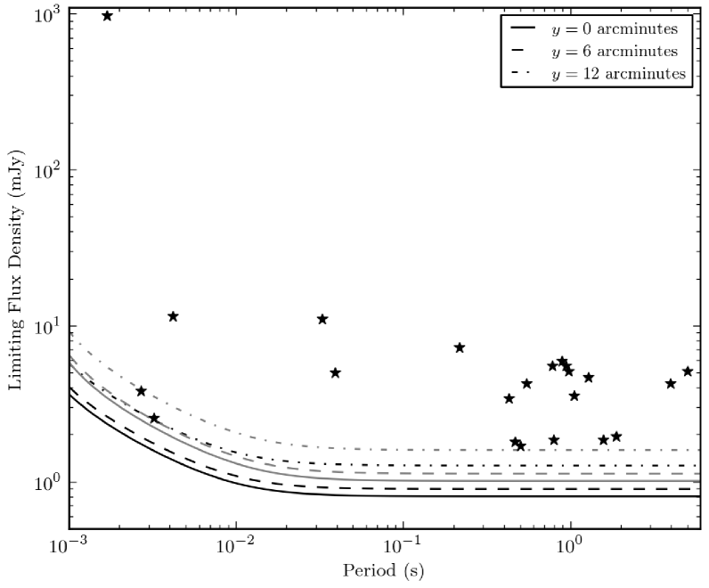
Figure 1: Approximate phase-averaged limiting flux density of our survey. Black curves are for $T_{\mathrm{sys}}=75\;\textrm{K}$ and $\textrm{DM}=30\;\mathrm{pc\;cm^{-3}}$, while gray curves are for $T_{\mathrm{sys}}=100\;\textrm{K}$ and $\textrm{DM}=75\;\mathrm{pc\;cm^{-3}}$. The smallest offset from the center of the telescope beam is $y$.

The system temperature is a sum of several factors, including the receiver temperature ($T_{\mathrm{rec}}$) and the sky temperature ($T_{\mathrm{sky}}$). The $350\;\textrm{MHz}$ receiver of the GBT has a nominal $T_{\mathrm{rec}}=23\;\textrm{K}$. The Galactic synchrotron emission contributes heavily to $T_{\mathrm{sky}}$, but this depends on sky position. Most of our survey was at high Galactic latitudes, where the synchrotron emission adds $\sim$30–$50\;\textrm{K}$ at $350\;\textrm{MHz}$ (Haslam et al., 1982). Our line of sight through the Galaxy also affects our sensitivity by increasing scattering and dispersion, both of which contribute to the observed pulse width. The typical maximum predicted DM at the high Galactic latitudes we cover is $\sim$$60\;\mathrm{pc\;cm^{-3}}$. According to the NE2001 model, this corresponds to a scattering time $\sim$$0.08\;\textrm{ms}$ at $350\;\textrm{MHz}$, though observed scattering times may differ from predictions by an order of magnitude or more. Obviously, DM effects become much worse at low Galactic latitudes. Figure 1 shows approximate sensitivity curves for various combinations of $y$ (the minimum offset from the beam center), $T_{\mathrm{sys}}$, and DM. These calculations do not take the effects of RFI into account, but as we describe in §2.1, the survey did not suffer greatly from RFI contamination.

4 Candidate Confirmation and Follow-up

Periodic and single-pulse candidates from each pseudo-pointing were judged by eye. Folded candidates were usually judged on three main criteria: i) distinct peaking of the signal’s significance at DMs greater than $0\;\mathrm{pc\;cm^{-3}}$; ii) broad-band emission (allowing for the possibility of regions of enhanced/diminished flux due to interstellar scintillation); and iii) fairly persistent emission in time (allowing for eclipses and nulls and accounting for the roll-off in sensitivity near the edges of the telescope beam). In the case of single-pulse candidates, we looked for pulses that peaked at a non-zero DM and that decreased in significance away from this peak. Multiple single pulses at the same DM were also an obvious indicator of a good candidate.

Promising candidates were confirmed in follow-up observations with the GBT, after which we began regular timing observations. To improve the quality of initial timing solutions, new pulsars had their sky positions refined by observing at a grid of locations with smaller GBT beams at successively higher frequencies (Morris et al., 2002). We used a number of dense observations early in the campaigns to characterize the orbits of binary pulsars. The majority of timing observations were carried out at $820\;\textrm{MHz}$, but most pulsars were also observed at other frequencies, allowing us to explore their spectral properties. We also started using the new Green Bank Ultimate Pulsar Processing Instrument (GUPPI) (DuPlain et al., 2008) in 2008 October. Compared to the Spigot back-end, GUPPI offers larger bandwidth, better frequency and time resolution, higher dynamic range, and greater resilience to strong RFI.

4.1 Pulsar Timing Analysis

All of the new pulsars were observed regularly with the GBT as part of our timing campaign. Long period pulsars (with $P>0.1\;\textrm{s}$) were observed for a minimum of about 11 months, while MSPs and recycled pulsars were observed for a minimum of 20. Each pulsar was typically observed for $10$–$15\;\min$ per observing session. High-S/N average pulse profiles were created for each observing frequency by summing data from multiple observations. We created standard pulse profiles by fitting one or more Gaussians to these average pulse profiles using a least squares minimization routine. These standard profiles were used to compute pulse times of arrival (TOAs) using either PRESTO or PSRCHIVE (Hotan et al., 2004) (depending on data format) by cross-correlation in the Fourier domain. We typically obtained two TOAs per observation for isolated pulsars and four to six TOAs per observation for binary pulsars, ensuring good sampling of the orbit. Phase connected timing solutions were created using the TEMPO software package and the DE405 Solar System ephemeris. All of our timing solutions are referenced to UTC(NIST). All the pulsars timed here have timing solutions with reduced $\chi^{2}>1$. Since we observe no unmodeled trends in our timing residuals, this is probably due to an underestimate of individual TOA uncertainties. As is standard practice, we multiplied all TOA uncertainties by an “error factor”, such that the reduced $\chi^{2}=1$.

4.2 Flux Measurements

Mean flux densities were estimated by assuming that the off-pulse root-mean-square (RMS) noise level was described by the radiometer equation,

$$\sigma=\frac{\beta T_{\mathrm{sys}}}{G\sqrt{n_{\mathrm{p}}\Delta\nu\,t_{\mathrm{int}}}},$$ (7)

where $T_{\mathrm{sys}}$ is the total system temperature. To ensure a proper estimate of the RMS noise level, we fit a third order polynomial to the off-pulse region and then subtracted this to create a flat off-pulse baseline. It is important to keep in mind, however, that observed pulsar fluxes are variable due to interstellar scintillation. The values that we report here are determined by averaging several observations but should be treated only as representative. We also calculated the spectral index when flux density estimates were available for multiple frequencies. We did this by fitting a standard power law to the flux density estimates, typically at $350\;\textrm{MHz}$ and $820\;\textrm{MHz}$, assuming $S_{\nu}\propto\nu^{\alpha}$. The average for the pulsars presented here is $\langle\alpha\rangle=-1.7$, which is very similar to the average value presented in Lorimer et al. (1995).

We also attempted to measure the rotation measure (RM) whenever fully calibrated polarization data were available (which was at least once for each pulsar). We searched over a wide range of RMs, from $\pm 1000\;\mathrm{rad\;\mathrm{m^{-2}}}$. We could only detect a significant RM for a subset of pulsars. Those pulsars without reported RMs are probably weakly polarized sources.

5 Results

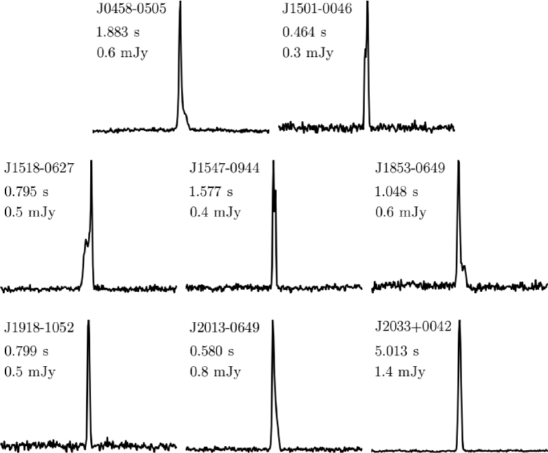
Figure 2: Integrated $820\;\textrm{MHz}$ pulse profiles for the newly discovered long period pulsars presented here. All profiles show one full rotation of the pulsar (i.e., from phase 0–1) with 256 phase bins. The profiles were made by adding all the RFI-free observations for each pulsar and were used to create standard pulse profiles at $820\;\textrm{MHz}$. Pulse periods and mean flux densities are also given.

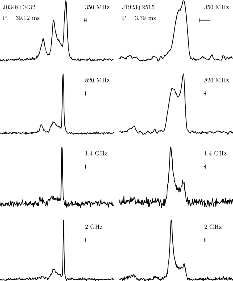
Figure 3: Integrated pulse profiles at four observing frequencies for the newly discovered recycled pulsars presented here. All profiles show one full rotation of the pulsar (i.e., from phase 0–1) with 256 phase bins. The summed profiles were made by aligning each folded profile using the TEMPO ephemeris and then adding all the RFI-free observations at the specified frequencies. The profile evolution in both pulsars is clear. The bars show the relative timescale for dispersive smearing at each frequency (see Equation 3).

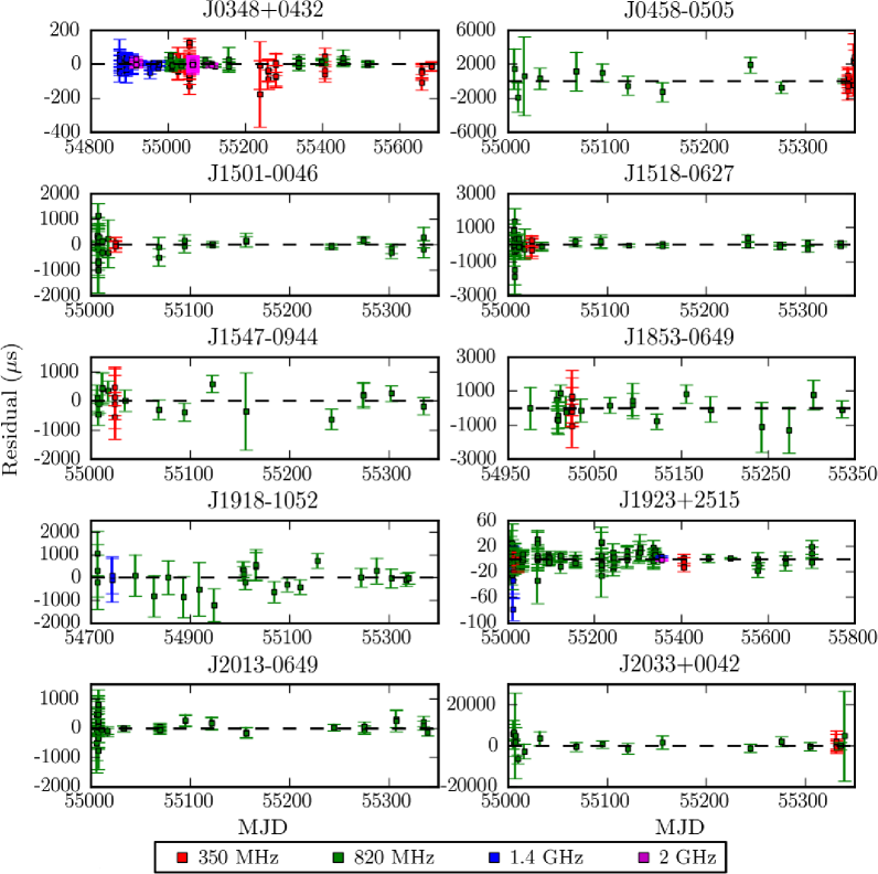
Figure 4: Post-fit timing residuals for each of the newly discovered pulsars. Only phase connected TOAs are shown. Nominal TOA errors have been multiplied by a constant error factor so that the reduced $\chi^{2}=1$. Note that the axes have different scales in most plots.

A total of 31 new pulsars have been discovered thus far in the Drift-scan Survey. The first 13 are presented in Paper I and 10 are discussed here. As mentioned in §1, PSR J1023$+$0038 has been discussed elsewhere by (Archibald et al., 2009) and (Archibald et al., 2010), while another MSP, PSR J2256$-$1024, will be presented in a future paper (Stairs et al. in prep). Full timing solutions have not been obtained for the six most recently discovered pulsars and these will be presented in future work. The 10 pulsars presented here include eight long period, isolated pulsars, one mildly recycled binary pulsar, and one isolated MSP. Seven of these 10 pulsars were detected independently in our searches for single pulses. Full timing solutions and other properties for the long-period pulsars are presented in Table 2 and for the recycled pulsars in Table 3. Integrated pulse profiles can be seen in Figures 2 and 3 and post-fit timing residuals are shown in Figure 4. We discuss some individual systems in greater detail below.

5.1 PSR J0348$+$0432: A Relativistic Binary with a Low-Mass Companion

PSR J0348$+$0432 (hereafter J0348) is a mildly recycled binary pulsar with $P=39.1\;\textrm{ms}$. The low magnetic field of J0348 ($B_{\mathrm{surf}}=3.1\times 10^{9}\;\textrm{G}$) indicates that it is indeed partially recycled and not a young pulsar. The DM of J0348 is $40.5\;\mathrm{pc\;cm^{-3}}$ and the DM-derived distance is $2.1\;\textrm{kpc}$. The orbital period of this system is $2.4\;\textrm{hr}$, and only three pulsars with $P<40\;\textrm{ms}$ outside of globular clusters have shorter periods. If we assume a mass of $1.4\;\mathrm{M_{\sun}}$ for J0348 then the observed mass function, $f(M)=2.9\times 10^{-4}$, implies a minimum companion mass of $0.086\;\mathrm{M_{\sun}}$. We searched for and identified an optical counterpart to J0348 in the Sloan Digital Sky Survey with corrected SDSS magnitudes $u^{\prime}=21.84\pm 0.19$, $g^{\prime}=20.71\pm 0.03$, $r^{\prime}=20.60\pm 0.03$, $i^{\prime}=20.69\pm 0.05$, and $z^{\prime}=20.40\pm 0.15$. More detailed spectroscopic follow-up with the Apache Point $3.5$-m telescope and the Very Large Telescope have shown that the companion to J0348 is a low-mass white dwarf. The combination of a neutron star and low-mass white dwarf in a tight, relativistic orbit is unique among pulsars and makes J0348 an excellent laboratory for testing general relativity and other theories of gravity. Specifically, theories that invoke a scalar gravitational field predict that J0348 will be a strong emitter of dipolar gravitational radiation because the very different binding energies of the neutron star and white dwarf will lead them to couple differently to the scalar field (e.g. Stairs, 2003). Similar tests have been done with PSR J1141$-$6545 (Bhat et al., 2008), J1012$+$5307 (Lazaridis et al., 2009) and J1738$+$0333 (Freire et al., 2012), but J0348 is in a tighter, more relativistic orbit and likely has a less massive companion, so it will be a stronger probe of these effects. A full analysis of the spectroscopic observations of J0348 and their implications for alternative theories of gravity will be presented in Antoniadis et al. (in prep).

J0348 shows significant profile evolution as a function of frequency (see Figure 3); at frequencies above $1.4\;\textrm{GHz}$, the main profile component becomes extremely narrow, with a duty cycle of $\sim$$1\%$. This has allowed us to obtain very precise pulse arrival times—our RMS timing residuals are $9.3\;\mathrm{\mu s}$ but at high frequencies individual TOA uncertainties can be $\lesssim 3\;\mathrm{\mu s}$. We are continuing long-term timing of this pulsar using the Arecibo Observatory.

5.2 PSR J1923$+$2515

PSR J1923$+$2515 (hereafter J1923) is an isolated MSP with a $3.8$-ms spin period. Figure 3 shows the integrated pulse profile of J1923 at several different frequencies and the evolution in the profile shape is clear. We see evidence for a weak interpulse in our summed $820\;\textrm{MHz}$ and $2\;\textrm{GHz}$ data. The timing of J1923 improved significantly at higher frequencies, where we were able to obtain TOAs with uncertainties $\lesssim 1\;\mathrm{\mu s}$. J1923 is being regularly observed at Arecibo as part of the NANOGrav timing array for gravitational wave detection (Demorest et al., 2012). It will also be suitable for the European Pulsar Timing Array (van Haasteren et al., 2011).

J1923 is the only pulsar presented here for which we were able to measure a significant proper motion. We find $\mu_{\alpha}=-6.2(1.2)\;\mathrm{mas}\,\mathrm{yr^{-1}}$ and $\mu_{\delta}=-23.6(3.5)\;\mathrm{mas}\,\mathrm{yr^{-1}}$. We performed an F-test to determine if the addition of proper motion is in fact required by the data. The full $\chi^{2}$ of our timing model excluding proper motion is 339.63, with 147 degrees of freedom. When proper motion is included in the fit, $\chi^{2}=146.02$ with 145 degrees of freedom. The probability that this improvement is due to chance is $1\times 10^{-16}$. Thus, the improvement in our timing solution when proper motion is included is extremely significant. We used the DM and the NE2001 model of Galactic free electron density to estimate the distance to J1923, $D=1.6(3)\;\textrm{kpc}$, where the number in parentheses represents a 20% fractional error, which is typical for these estimates (Cordes & Lazio, 2002). At this distance, the observed proper motion corresponds to a transverse velocity $v_{\perp}=188(46)\;\textrm{km}\,\mathrm{s^{-1}}$, which is within the observed range of other MSPs, though higher than average (Gothoskar & Gupta, 2000; Bogdanov et al., 2002; Gonzalez et al., 2011).

Using this $v_{\perp}$ we can calculate the magnitude of the Shklovskii effect (Shklovskii, 1970):

$$\frac{\dot{P}_{\mu}}{P}=\frac{v_{\perp}^{2}}{c\;D}.$$ (8)

We find $\dot{P}_{\mu}=8.9(4.7)\times 10^{-21}\;\textrm{s}\,\mathrm{s^{-1}}$. Acceleration within the Galactic potential will also cause a bias in the observed $\dot{P}$. We estimate this contribution following Nice & Taylor (1995), but find that biases due to acceleration perpendicular and parallel to the Galactic plane are only $-3.3\times 10^{-22}\;\textrm{s}\,\mathrm{s^{-1}}$ and $-3.4\times 10^{-22}\;\textrm{s}\,\mathrm{s^{-1}}$, respectively. These are an order of magnitude smaller than $\dot{P}_{\mu}$. The bias due to the Shklovskii effect is 94% of the observed $\dot{P}$ and would imply that the intrinsic spin-down of the pulsar is $\dot{P}_{\mathrm{int}}=0.6(4.7)\times 10^{-21}\;\textrm{s}\,\mathrm{s^{-1}}$, so we can only place an upper limit on $\dot{P}_{\mathrm{int}}$ at this time. A more precise measurement of proper motion or a better distance estimate will be needed to constrain the magnitude of the Shklovskii effect and to obtain a better measurement of $\dot{P}_{\mathrm{int}}$. In the meantime, the derived quantities listed in Table 3 are upper limits based upon our measurement uncertainties for $\dot{P}_{\mathrm{int}}$.

5.3 PSR J0458$-$0505

PSR J0458$-$0505 (hereafter J0458) is a nulling pulsar with a $1.9$-s spin period. It was detected in both the Fourier domain and single-pulse searches. The profile is slightly asymmetric (see Figure 2), with a small trailing component. The reduced $\chi^{2}$ obtained from our timing solution after fitting for position, $P$, $\dot{P}$, and DM was substantially higher than unity. As we see no systematic trends in our timing residuals, we assume that the number of pulses per individual observation was too small, due to a combination of a long period, limited integration time and a very large nulling fraction (see below). The pulse profile thus probably did not stabilize within these TOA integrations. To make the reduced $\chi^{2}$ equal to one, we multiplied our individual TOA errors by a constant factor of $2.97$. Although we were still able to derive an accurate timing solution for J0458, the fractional errors in the timing parameters are larger than for most of the other pulsars presented here, especially for declination and $\dot{P}$.

5.3.1 Estimate of the Nulling Fraction

We estimate the nulling fraction, NF, of J0458 in the following way. We first removed strong sources of RFI from each observation. We then folded each data-set using sub-integrations that were a single pulse period in duration using the psrfits_singlepulse command from psrfits_utils. In some sub-integrations, systematic trends due to lower levels of RFI were still visible. To remove these, we used a least-squares minimization technique to fit up to a maximum of four independent sinusoids to the off-pulse region of each sub-integration and then subtracted them from the data, creating a flat off-pulse baseline. Each sub-integration was then normalized to have an off-pulse median and RMS noise level of zero and one, respectively.

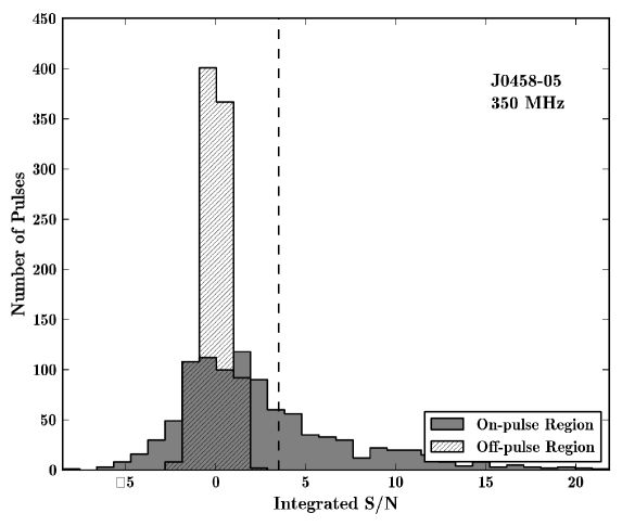
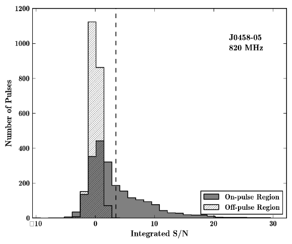
Figure 5: Histograms of integrated S/N for single pulses of J0458. The top panel is for data taken at $350\;\textrm{MHz}$, while the bottom panel is for data taken at $820\;\textrm{MHz}$. The on-pulse region is shown in gray and the off-pulse region as hatched. The dashed line shows the $\textrm{S/N}_{\mathrm{thresh}}=3.5$, above which we counted the pulsar as being in an “on” state.

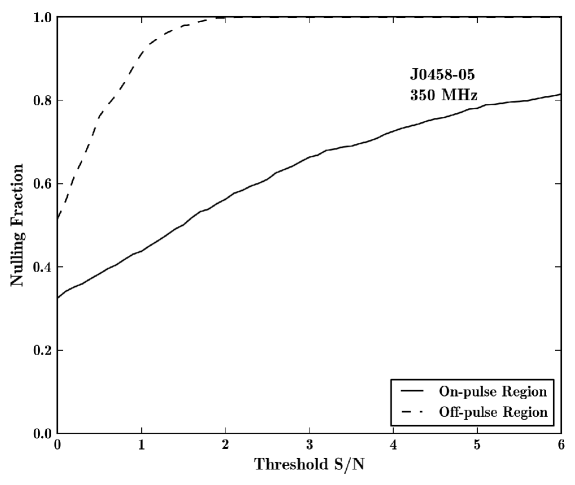
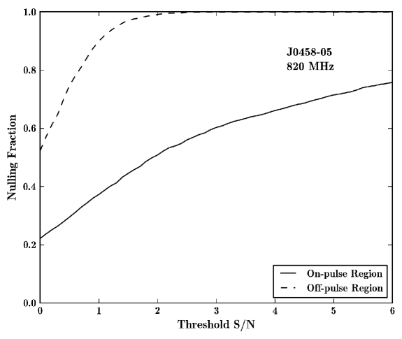
Figure 6: The nulling fraction of J0458 as a function of $\textrm{S/N}_{\mathrm{thresh}}$. The top panel is for data taken at $350\;\textrm{MHz}$, while the bottom panel is for data taken at $820\;\textrm{MHz}$.

To determine if the pulsar was in an “on” state, we calculated the integrated S/N in the on-pulse region, which was determined by inspection of the integrated pulse profile. We also calculated the integrated S/N in an off-pulse region with the same number of bins as the on-pulse region. We counted a pulse as being in the “on” state if it had an integrated S/N above some threshold, $\textrm{S/N}_{\mathrm{thresh}}$. We chose $\textrm{S/N}_{\mathrm{thresh}}$ based on the statistics of the off-pulse region. Histograms of the on-pulse and off-pulse S/Ns can be found in Figure 5 and in Figure 6 we show NF as a function of threshold S/N. Our calculations show that the off-pulse region rarely exceeded $\textrm{S/N}=3.0$, as expected for Gaussian distributed noise. To be conservative, we set $\textrm{S/N}_{\mathrm{thresh}}=3.5$, though we also report NF for $\textrm{S/N}_{\mathrm{thresh}}=3.0$ and $4.0$ for comparison.

After removing RFI, J0458 was observed for a total of 2218 full rotations at $820\;\textrm{MHz}$ and we find $\mathrm{NF}=[0.60,0.63,0.66]$ for $\textrm{S/N}_{\mathrm{thresh}}=[3.0,3.5,4.0]$, respectively. J0458 was observed for a total of 978 rotations at $350\;\textrm{MHz}$ with $\mathrm{NF}=[0.66,0.69,0.73]$ for $\textrm{S/N}_{\mathrm{thresh}}=[3.0,3.5,4.0]$, respectively. These $\mathrm{NFs}$ are fairly high compared to other pulsars, but are not unprecedented — PSRs B1112+50 and B1944+17 have comparable $\mathrm{NF}$ (Ritchings, 1976). The nulling fraction of J0458 seems to be similar at both $350\;\textrm{MHz}$ and $820\;\textrm{MHz}$. This behavior is consistent with previous studies that suggest nulling is a broadband phenomenon at low frequencies (see Biggs, 1992, and references therein).

5.4 PSR J2033$+$0042

PSR J2033$+$0042 (hereafter J2033) is a $5.0$-s pulsar that, like J0458, nulls significantly. It was reported by Burke-Spolaor & Bailes (2010) as a RRAT that sometimes was detected in Fourier searches. Burke-Spolaor & Bailes (2010) report on the position, period, and DM of J2033 and note its high nulling fraction and the presence of drifting sub-pulses. Here, we present a full timing solution and quantitative measurement of the nulling fraction. We detected J2033 in both single-pulse and Fourier searches. Only nine radio pulsars and 12 RRATs in the ATNF catalog have a longer period than J2033. Like J0458, the fractional errors in our timing parameters were relatively large, probably because our integration times were shorter than the pulse stabilization time. J2033 has a longer period than J0458 and also nulls significantly.

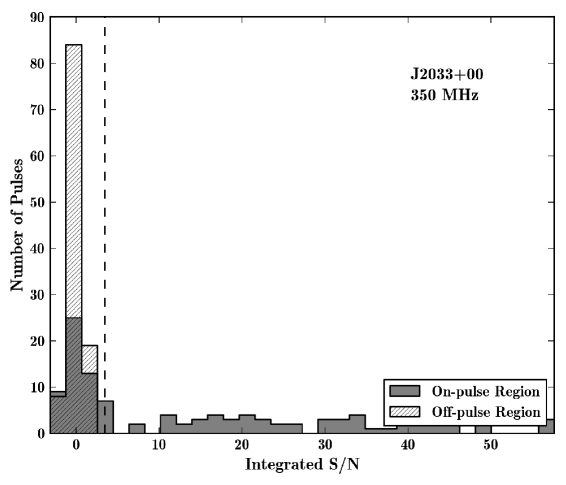
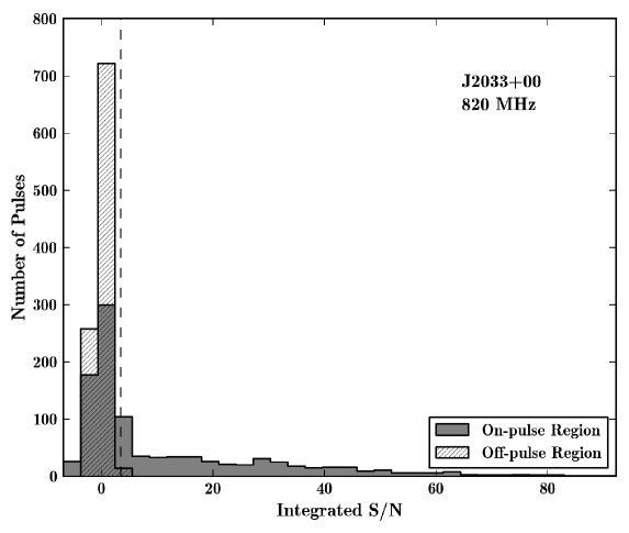
Figure 7: Histograms of S/N for single pulses of J2033. The data labels are the same as in Figure 5.

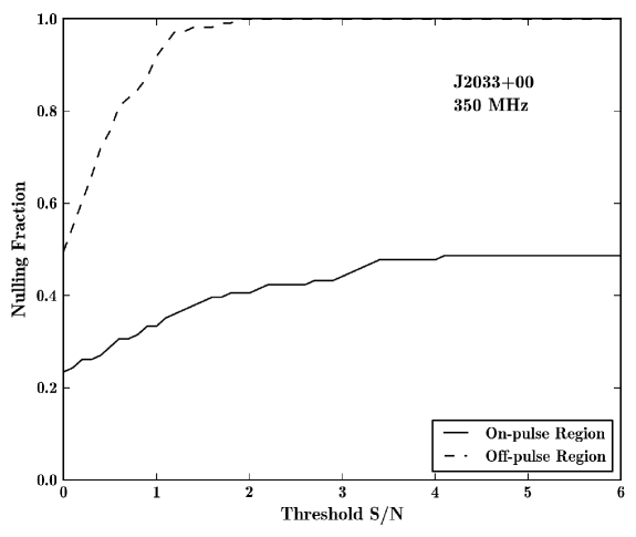
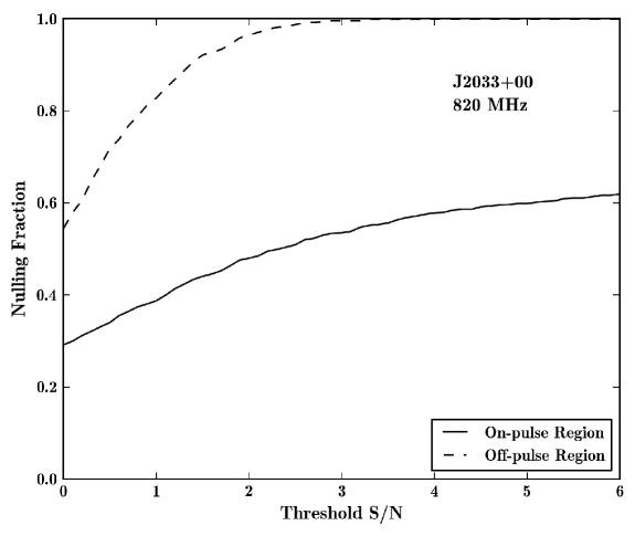
Figure 8: The nulling fraction of J2033 as a function of $\textrm{S/N}_{\mathrm{thresh}}$. The data labels are the same as in Figure 6.

We used the same procedure as outlined in §5.3.1 to estimate the nulling fraction in J2033. We observed the pulsar for 994 rotations at $820\;\textrm{MHz}$ and we find a $\mathrm{NF}=[0.53,0.56,0.58]$ for $\textrm{S/N}_{\mathrm{thresh}}=[3.0,3.5,4.0]$, respectively. J2033 was observed for 111 rotations at $350\;\textrm{MHz}$ and we find $\mathrm{NF}=[0.44,0.48,0.49]$ for $\textrm{S/N}_{\mathrm{thresh}}=[3.0,3.5,4.0]$, respectively. Histograms of S/N can be found in Figure 7 and $\mathrm{NF}$ as a function of $\textrm{S/N}_{\mathrm{thresh}}$ is plotted in Figure 8. The nulling fraction of J2033 is somewhat higher at $820\;\textrm{MHz}$ than at $350\;\textrm{MHz}$, but we only observed J2033 at $350\;\textrm{MHz}$ on one occasion, so a more detailed study of the nulling characteristics of this pulsar should be conducted before drawing firm conclusions about the frequency dependence of $\mathrm{NF}$. Overall, pulsars J0458 and J2033 are on less than half of the time, adding to a growing sub-population of pulsars that are mostly off (Keane et al., 2011).

6 Conclusion

The Drift-scan Survey has discovered 31 pulsars, of which 10 are presented here. The majority are isolated long-period pulsars. J0348 is a mildly recycled binary pulsar that has a low-mass white dwarf companion in a relativistic orbit. It is a unique and powerful system for testing gravitational theories and hence we are continuing to time it long-term. A more detailed study of J0348 will be presented in Antoniadis et al. (in prep). J1923 is an isolated MSP. We have a significant measurement of the pulsar’s proper motion, but the implied magnitude of the Shklovskii effect is nearly equal to the observed spin-down, so we are only able to set limits on the rotational characteristics of J1923. Long-term monitoring should help to better constrain the proper motion and intrinsic spin-down. J0458 and J2033 are both nulling pulsars with nulling fractions $\gtrsim 50\%$.

R.S.L. was a student at the National Radio Astronomy Observatory and was supported through the GBT Student Support program and the National Science Foundation grant AST-0907967 during the course of this work. D.R.L., M.A.M., and J.B. acknowledge support from a WVEPSCoR Research Challenge Grant. J.W.T.H. is a Veni Fellow of the Netherlands Foundation for Scientific Research. Pulsar research at UBC is supported by an NSERC Discovery Grant and Special Research Opportunity grant as well as the Canada Foundation for Innovation. V.M.K. holds the Lorne Trottier Chair in Astrophysics and Cosmology, and a Canada Research Chair, a Killam Research Fellowship, and acknowledges additional support from an NSERC Discovery Grant, from FQRNT via le Centre de Recherche Astrophysique du Quebéc and the Canadian Institute for Advanced Research. R.F.C., C.E.R., and T.P. were summer students at the National Radio Astronomy Observatory during a portion of this work. We thank Paulo Freire for refereeing this manuscript and providing helpful feedback. We are also grateful to NRAO for a grant that assisted data storage. The National Radio Astronomy Observatory is a facility of the National Science Foundation operated under cooperative agreement by Associated Universities, Inc.

Table 1: Parameters of the GBT $350\;\textrm{MHz}$ Drift-scan Survey

Paramter	Value
ADC Conversion Factor, $\beta$	1.16
Signal-to-noise threshhold, $\textrm{S/N}_{\mathrm{min}}$	6.0
Receiver Temperature, $T_{\mathrm{rec}}$ (K)	46
Telescope Gain, $G$ ($\textrm{K}\;\textrm{Jy}^{-1}$)	2.0
Number of summed polarizations, $n_{\mathrm{p}}$	2
Length of pseudo-pointing, $t_{\mathrm{int}}$ (s)	140
Bandwidth, $\Delta f$ (MHz)	50
Number of frequency channels, $n_{\mathrm{chan}}$	2048
Sampling time, $t_{\mathrm{samp}}$ ($\mathrm{\mu s}$)	81.92

Table 2: Parameters of Newly Discovered Long Period Pulsars

Parameter	PSR J0458$-$0505	PSR J1501$-$0046	PSR J1518$-$0627
Timing Parameters
Right Ascension (J2000)	04:58:37.121(26)	15:01:44.9558(94)	15:18:59.1104(80)
Declination (J2000)	$-$05:05:05.1(4.0)	$-$00:46:23.52(88)	$-$06:27:07.70(66)
Pulsar Period (s)	1.88347965849(18 )	0.4640368139284(82)	0.7949966745699(78)
Period Derivative ($\textrm{s}\,\mathrm{s^{-1}}$)	5.3(1.5)$\times$10-16	2.391(60)$\times$10-16	4.179(56)$\times$10-16
Dispersion Measure ($\mathrm{pc\;cm^{-3}}$)	47.806(32)	22.2584(90)	27.9631(98)
Reference Epoch (MJD)	55178.0	55170.0	55170.0
Span of Timing Data (MJD)	55006–55349	55006–55335	55006–55335
Number of TOAs	22	39	43
RMS Residual ($\mathrm{\mu s}$)	716	172	175
Error Factor	2.967	1.095	1.050
Derived Parameters
Galactic Longitude (deg)	204.14	356.58	355.15
Galactic Latitude (deg)	$-$27.35	48.05	41.0
DM Derived Distance (kpc)	2.6	1.4	1.6
Surface Magnetic Field ($10^{12}$ Gauss)	1.0	0.33	0.58
Spin-down Luminosity ($10^{32}\;\textrm{erg}\,\mathrm{s^{-1}}$)	0.032	0.95	0.33
Characteristic Age (Myr)	56	31	30
$820\;\textrm{MHz}$ FWHM	0.014	0.022	0.012
$820\;\textrm{MHz}$ Flux Density (mJy)	0.5	0.3	0.4
Spectral Index	$-1.6$	$-2.1$	$-1.8$

Table 2: Parameters of Newly Discovered Long Period Pulsars (Cont.)

Parameter	PSR J1547$-$0944	PSR J1853$-$0649	PSR J1918$-$1052
Timing Parameters
Right Ascension (J2000)	15:47:46.058(36)	18:53:25.422(36)	19:18:48.247(13)
Declination (J2000)	$-$09:44:7.8(3.2)	$-$06:49:25.9(2.6)	$-$10:52:46.38(66)
Pulsar Period (s)	1.576924632943(44)	1.048132105087(54)	0.798692542358(15)
Period Derivative ($\textrm{s}\,\mathrm{s^{-1}}$)	2.938(36)$\times$10-15	1.548(44)$\times$10-15	8.653(15)$\times$10-16
Dispersion Measure ($\mathrm{pc\;cm^{-3}}$)	37.416(22)	44.541(36)	62.73(80)
Reference Epoch (MJD)	55170.0	55170.0	55026.0
Span of Timing Data (MJD)	55006–55335	54976–55335	54712–55339
Number of TOAs	22	24	26
RMS Residual ($\mathrm{\mu s}$)	338	588	394
Error Factor	1.630	2.150	2.480
Derived Parameters
Galactic Longitude (deg)	358.31	27.08	26.23
Galactic Latitude (deg)	33.57	$-$3.55	$-$10.96
DM Derived Distance (kpc)	1.9	1.5	2.1
Surface Magnetic Field ($10^{12}$ Gauss)	2.2	1.3	0.84
Spin-down Luminosity ($10^{32}\;\textrm{erg}\,\mathrm{s^{-1}}$)	0.30	0.53	0.67
Characteristic Age (Myr)	8.5	11	15
$820\;\textrm{MHz}$ FWHM	0.019	0.015	0.015
$820\;\textrm{MHz}$ Flux Density (mJy)	0.4	0.5	0.4
Spectral Index	$-1.8$	$-2.3$	$\cdots$
Rotation Measure ($\mathrm{rad}\,\mathrm{m^{-2}}$)	$\cdots$	34.7(3.2)	$-47.6(6.0)$

Table 2: Parameters of Newly Discovered Long Period Pulsars (Cont.)

Parameter	PSR J2013$-$0649	PSR J2033+0042
Timing Parameters
Right Ascension (J2000)	20:13:17.7507(38)	20:33:31.11(12)
Declination (J2000)	$-$06:49:05.39(32)	00:42:22.0(8.0)
Pulsar Period (s)	0.5801872690010(34)	5.01339800063(90)
Period Derivative ($\textrm{s}\,\mathrm{s^{-1}}$)	6.007(24)$\times$10-16	1.013(78)$\times$10-14
Dispersion Measure ($\mathrm{pc\;cm^{-3}}$)	63.36(10)	37.84(13)
Reference Epoch (MJD)	55172.0	55172.0
Span of Timing Data (MJD)	55005–55339	55005–55339
Number of TOAs	45	22
RMS Residual ($\mathrm{\mu s}$)	150	2195
Error Factor	1.370	4.680
Derived Parameters
Galactic Longitude (deg)	36.17	45.88
Galactic Latitude (deg)	$-$21.29	$-$22.2
DM Derived Distance (kpc)	3.0	1.9
Surface Magnetic Field ($10^{12}$ Gauss)	0.60	7.2
Spin-down Luminosity ($10^{32}\;\textrm{erg}\,\mathrm{s^{-1}}$)	1.2	0.032
Characteristic Age (Myr)	15	7.8
$820\;\textrm{MHz}$ FWHM	0.017	0.018
$820\;\textrm{MHz}$ Flux Density (mJy)	0.6	1.2
Spectral Index	$\cdots$	$-1.7$
Rotation Measure ($\mathrm{rad}\,\mathrm{m^{-2}}$)	$\cdots$	$-71.2(2.2)$

Note. — Numbers in parentheses are 1-$\sigma$ uncertainties as determined by TEMPO; although we have scaled the TOA uncertainties by the error factors reported, we have not doubled the nominal TEMPO uncertainties as is sometimes done in these cases. Flux density estimates typically have a 20–30% relative uncertainty due to scintillation. All timing solutions use the DE405 Solar System Ephemeris and the UTC(NIST) time system. Derived quantities assume an $R=10\;\textrm{km}$ neutron star with $I=10^{45}\;\textrm{gm}\,\textrm{cm}^{2}$ (see Lorimer & Kramer, 2005). The DM derived distances were calculated using the NE2001 model of Galactic free electron density, and have typical errors of $\sim 20\%$ (Cordes & Lazio, 2002).

Table 3: Parameters of Newly Discovered Short Period Pulsars

Parameter	PSR J0348+0432	PSR J1923+2515
Timing Parameters
Right Ascension (RA; J2000)	03:48:43.63817(33)	19:23:22.494560(76)
Declination (DEC; J2000)	04:32:11.449(10)	25:15:40.6436(14)
RA Proper Motion ($\mathrm{mas}\,\mathrm{yr^{-1}}$)	$\cdots$	$-$6.2(2.4)
DEC Proper Motion ($\mathrm{mas}\,\mathrm{yr^{-1}}$)	$\cdots$	$-$23.5(7.0)
Pulsar Period (s)	0.039122656280156(10)	0.00378815551961303(52)
Period Derivative ($\textrm{s}\,\mathrm{s^{-1}}$)	2.417(16)$\times$10-19	9.42(14)$\times$10-21
Dispersion Measure ($\mathrm{pc\;cm^{-3}}$)	40.56(11)	18.85766(19)
Reference Epoch (MJD)	55278.0	55322.0
Span of Timing Data (MJD)	54873–55682	55005–55639
Number of TOAs	183	153
Error Factor	1.657	1.245
RMS Residual ($\mathrm{\mu s}$)	10.33	5.0
Binary Parameters
Binary Model	ELL1	$\cdots$
Orbital Period (days)	0.10242406134(30)	$\cdots$
Projected Semi-major Axis (lt-s)	0.1409842(34)	$\cdots$
Epoch of Ascending Node (MJD)	54889.70532337(65)	$\cdots$
1st Laplace Parameter	$<5.0\times 10^{-5}$	$\cdots$
2nd Laplace Parameter	$<6.3\times 10^{-5}$	$\cdots$
Derived Parameters
Orbital Eccentricity	$<8.1\times 10^{-5}$	$\cdots$
Mass Function ($\mathrm{M_{\sun}}$)	0.000286807(20)	$\cdots$
Minimum Companion Mass ($\mathrm{M_{\sun}}$)	0.086	$\cdots$
Galactic Longitude (deg)	183.34	58.95
Galactic Latitude (deg)	$-$36.77	4.75
DM Derived Distance (kpc)	2.1	1.6
Transverse Velocity ($\textrm{km}\,\mathrm{s^{-1}}$)	$\cdots$	188(46)
Shklovskii Effect ($\textrm{s}\,\mathrm{s^{-1}}$)	$\cdots$	8.9(4.7)$\times$10-21
Intrinsic Spin-down ($\textrm{s}\,\mathrm{s^{-1}}$)	$\cdots$	$<5.3\times 10^{-21}$
Surface Magnetic Field ($10^{9}$ Gauss)	3.1	$<1.4$
Spin-down Luminosity ($10^{32}\;\textrm{erg}\,\mathrm{s^{-1}}$)	1.6	$<38$
Characteristic Age (Gyr)	2.6	$>11$
$820\;\textrm{MHz}$ FWHM	0.016	0.142
$820\;\textrm{MHz}$ Flux Density (mJy)	1.8	0.6
Spectral Index	$-1.2$	$-1.7$
Rotation Measure ($\mathrm{rad}\,\mathrm{m^{-2}}$)	49.5(13)	10.8(3.8)

Note. — Numbers in parentheses are 1-$\sigma$ uncertainties as determined by TEMPO; although we have scaled the TOA uncertainties by the error factors reported, we have not doubled the nominal TEMPO uncertainties as is sometimes done in these cases. Flux density estimates typically have a 20–30% relative uncertainty due to scintillation. All timing solutions use the DE405 Solar System Ephemeris and the UTC(NIST) time system. Derived quantities assume an $R=10\;\textrm{km}$ neutron star with $I=10^{45}\;\textrm{gm}\,\textrm{cm}^{2}$ (see Lorimer & Kramer, 2005). Minimum companion masses were calculated assuming a $1.4\;\mathrm{M_{\sun}}$ pulsar. The DM derived distances were calculated using the NE2001 model of Galactic free electron density, and have typical errors of $\sim 20\%$ (Cordes & Lazio, 2002).

References

- Archibald et al. (2010) Archibald, A. M., Kaspi, V. M., Bogdanov, S., et al. 2010, ApJ, 722, 88
- Archibald et al. (2009) Archibald, A. M., Stairs, I. H., Ransom, S. M., et al. 2009, Science, 324, 1411
- Bhat et al. (2008) Bhat, N. D. R., Bailes, M., & Verbiest, J. P. W. 2008, Phys. Rev. D, 77, 124017
- Biggs (1992) Biggs, J. D. 1992, ApJ, 394, 574
- Bogdanov et al. (2002) Bogdanov, S., Pruszyńska, M., Lewandowski, W., & Wolszczan, A. 2002, ApJ, 581, 495
- Boyles et al. (2012) Boyles, J., Lynch, R. S., Lorimer, D. R., et al. 2012, ApJ, in prep
- Burke-Spolaor & Bailes (2010) Burke-Spolaor, S., & Bailes, M. 2010, MNRAS, 402, 855
- Cordes & Lazio (2002) Cordes, J. M., & Lazio, T. J. W. 2002, ArXiv Astrophysics e-prints astro-ph/0207156
- Demorest et al. (2012) Demorest, P. B., Ferdman, R. D., Gonzalez, M. E., et al. 2012, ArXiv e-prints 1201.6641
- Dewey et al. (1985) Dewey, R. J., Taylor, J. H., Weisberg, J. M., & Stokes, G. H. 1985, ApJ, 294, L25
- DuPlain et al. (2008) DuPlain, R., Ransom, S., Demorest, P., et al. 2008, in Society of Photo-Optical Instrumentation Engineers (SPIE) Conference Series, Vol. 7019, Society of Photo-Optical Instrumentation Engineers (SPIE) Conference Series, 70191D–70191D–10
- Freire et al. (2012) Freire, P. C. C., Wex, N., Esposito-Farèse, G., et al. 2012, MNRAS, 423, 3328
- Gonzalez et al. (2011) Gonzalez, M. E., Stairs, I. H., Ferdman, R. D., et al. 2011, ApJ, 743, 102
- Gothoskar & Gupta (2000) Gothoskar, P., & Gupta, Y. 2000, ApJ, 531, 345
- Haslam et al. (1982) Haslam, C. G. T., Salter, C. J., Stoffel, H., & Wilson, W. E. 1982, A&AS, 47, 1
- Hessels et al. (2008) Hessels, J. W. T., Ransom, S. M., Kaspi, V. M., et al. 2008, in American Institute of Physics Conference Series, Vol. 983, 40 Years of Pulsars: Millisecond Pulsars, Magnetars and More, ed. C. Bassa, Z. Wang, A. Cumming, & V. M. Kaspi, 613–615
- Hotan et al. (2004) Hotan, A. W., van Straten, W., & Manchester, R. N. 2004, PASA, 21, 302
- Jenet et al. (2009) Jenet, F., Finn, L. S., Lazio, J., et al. 2009, ArXiv e-prints 0909.1058
- Kaplan et al. (2005) Kaplan, D. L., Escoffier, R. P., Lacasse, R. J., et al. 2005, PASP, 117, 643
- Keane et al. (2011) Keane, E. F., Kramer, M., Lyne, A. G., Stappers, B. W., & McLaughlin, M. A. 2011, MNRAS, 415, 3065
- Lazaridis et al. (2009) Lazaridis, K., Wex, N., Jessner, A., et al. 2009, MNRAS, 400, 805
- Lorimer & Kramer (2005) Lorimer, D. R., & Kramer, M. 2005, Handbook of Pulsar Astronomy (Cambridge, UK: Cambridge University Press)
- Lorimer et al. (1995) Lorimer, D. R., Yates, J. A., Lyne, A. G., & Gould, D. M. 1995, MNRAS, 273, 411
- Morris et al. (2002) Morris, D. J., Hobbs, G., Lyne, A. G., et al. 2002, MNRAS, 335, 275
- Nice & Taylor (1995) Nice, D. J., & Taylor, J. H. 1995, ApJ, 441, 429
- Ransom (2001) Ransom, S. M. 2001, PhD thesis, Harvard University
- Ransom et al. (2002) Ransom, S. M., Eikenberry, S. S., & Middleditch, J. 2002, AJ, 124, 1788
- Ritchings (1976) Ritchings, R. T. 1976, MNRAS, 176, 249
- Rosen et al. (2010) Rosen, R., Heatherly, S., McLaughlin, M. A., et al. 2010, Astronomy Education Review, 9, 010106
- Shklovskii (1970) Shklovskii, I. S. 1970, Soviet Ast., 13, 562
- Stairs (2003) Stairs, I. H. 2003, Living Reviews in Relativity, 6, 5
- van Haasteren et al. (2011) van Haasteren, R., Levin, Y., Janssen, G. H., et al. 2011, MNRAS, 414, 3117