Tomographic characterisation of correlations in a photonic tripartite state

Abstract

Starting from a four-partite photonic hyper-entangled Dicke resource, we report the full tomographic characterization of three-, two-, and one-qubit states obtained by projecting out part of the computational register. The reduced states thus obtained correspond to fidelities with the expected states larger than $87\%$, therefore certifying the faithfulness of the entanglement-sharing structure within the original four-qubit resource. The high quality of the reduced three-qubit state allows for the experimental verification of the Koashi-Winter relation for the monogamy of correlations within a tripartite state. We show that, by exploiting the symmetries of the three-qubit state obtained upon projection over the four-qubit Dicke resource, such relation can be experimentally fully characterized using only 5 measurement settings. We highlight the limitations of such approach and sketch an experimentally-oriented way to overcome them.

1 Introduction

Linear optics is at the forefront of current experimental quantum information processing, providing settings, operations and states of outstanding quality, controllability and testability [1, 2]. Among many other achievements, the first test-bed demonstration of protocols for quantum teleportation [3, 4, 5], measurement-based quantum computation [6] and quantum-empowered communication [7] have been provided in linear optics setups. Very recently, some seminal proposals and demonstrations have been given of the suitability of bulk- as well as integrated-optics settings for the controllable simulation of quantum phenomena, including the properties of frustrated spin systems [8], the statistics of two-particle (correlated) quantum random walks [9], simple quantum games [10] and chemical processes [11]. Despite sounding visionary, the possibility of using photonic devices to simulate the properties of complex molecular and biological systems, as well the phenomenological features particle statistics and high-energy physics is rapidly affirming itself as a viable possibility of not-far-fetched experimental realization [12, 13].

Such an astonishing success is due to the reconfigurability of photonic interferometers and circuits, as well as the virtually noise-free, highly accurate reconstruction of the states that result from the performance of a quantum information protocol via quantum state tomography (QST) techniques [14]. Together with quantum process tomography [15], which aims at reconstructing the properties of an actual (unitary or non-unitary) quantum channel, QST has affirmed itself as the premier diagnostic tool in linear optics quantum information processing, allowing for the reconstruction of the density matrix describing the state of intricate multipartite quantum-correlated systems. Besides enabling the evaluation of the performance of most of the schemes mentioned above, QST has recently allowed for the exploration of quantum correlations beyond entanglement in two-qubit systems [16] and the experimental assessment of quantum discord [17, 18, 19] as a resource for quantum communication [20]. Further endeavours directed towards the experimental determination of discord in different physical systems have been reported recently . The experimental reconstruction of the state of a system, indeed, allows for the handy evaluation of figures of merit that are key to the characterization of the quality of information processing at the quantum level. Moreover, it embodies a useful tool for the evaluation of the limitations of a given experimental setup, thus contributing to the design and the improvement of the experimental protocol that the set-up is supposed to accommodate.

In this paper, we employ QST to accomplish a twofold task. First, we contribute to the current quest for the experimental generation and manipulation of complex multi-qubit entangled states [22, 23] by indirectly characterizing the entanglement-sharing structure within a four-qubit photonic resource prepared in a symmetric Dicke state with two excitations and encoded in the polarization and momentum degrees of freedom (DOFs) of an hyper-entangled state. Four and six-qubit photonic Dicke states have been experimentally generated and tested by means of ad hoc entanglement witnesses [24, 25]. Very recently, a four-qubit Dicke resource has been used as the computational register for the implementation of important protocols for quantum networking [27]. Our approach here will be to characterize the faithfulness of our Dicke-state generator by projecting out a growing number of elements of the computational register and testing the faithfulness of the reduced states thus generated to the expected ideal states. In particular, we report the experimental QST of three-qubit Dicke states with one and two excitations, as well as two-qubit (Bell) states and single-qubit ones. The values off the state fidelity associated with each family of projected states witnesses the closeness of the original quadripartite resource to the ideal Dicke one.

Our second task moves from the high quality of the three-qubit states generated as described above to address the monogamy of correlations within a tripartite state. In particular, we attack the celebrated relation formulated by Koashi and Winter in Ref. [28] and provide its experimental evaluation. In particular, we give a state-symmetry simplified expression for each entry of the Koashi-Winter (KW) relation and demonstrate that, for the class of three-qubit Dicke states (with one excitation), the latter can be experimentally tested by making use of only five measurements settings, which we have implemented in our experiment. We conclude our investigation by providing a plausible analysis of the reasons behind the deviations of the experimental value of the KW relation from the expected value.

The remainder of this paper is organized as follows. In Sec. 2 we introduce the quadripartite Dicke resource, describe the experimental apparatus used in order to encode such state in the hyper-entanglement of momentum and polarization of a photonic register and address the projection-based generation and tomographic reconstruction of the class of three, two and single-qubit states addressed above. In Sec. 7 we tackle the KW relation and its experimental verification over one of our three-qubit states. Besides providing the decomposition of such monogamy relation in terms of the correlators that can be measured through only five measurement settings, we highlight the effects of mixedness and anisotropy in its experimental evaluation, providing a KW-based estimate of the actual form of the experimentally projected three-qubit resource. Finally, in Sec. 4, we draw to our conclusions.

2 Experimental realization of a four-qubit Dicke resource and tomographic reconstruction of projected states

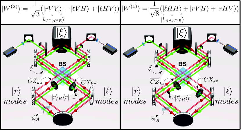
Figure 1: Experimental setup for the generation and analysis of three-qubit $|W^{(1,2)}\rangle$ states obtained from the projection of the momentum qubit $d$ of the quadripartite Dicke state $|D^{(2)}_{4}\rangle$ onto $|r\rangle$ (left panel) and $|\ell\rangle$ (right panel), respectively. The red (green) modes represent the optical path followed by photon A (B).

We used the experimental setup allowing to engineer a symmetric Dicke state by starting from a two photon four qubit polarization-momentum hyper-entangled state  [23], already exploited in  [25, 27, 26] to test multipartite entanglement, decoherence and general quantum correlations [16, 25]. In the following we use both polarization-qubit and path-qubit encoding, $\{|H\rangle,|V\rangle\}{\equiv}\{|0\rangle,|1\rangle\}$, $\{|r\rangle,|\ell\rangle\}{\equiv}\{|0\rangle,|1\rangle\}$, with $H/V$ corresponding to the horizontal/vertical polarization of a single photon, while $r$ and $\ell$ are the path followed by photons. The setup was suitably adjusted to prepare the state

$$|\xi\rangle_{abcd}{=}[|HH\rangle_{ab}(|r\ell\rangle-|\ell r\rangle)_{cd}+2|VV\rangle_{ab}|r\ell\rangle]_{cd}/\sqrt{6}.$$ (1)

Here, qubits $a,c$ ($b,d$) are encoded in the polarization and momentum of photon A (B). Eq. (1) can be easily turned into the four-qubit two-excitation Dicke state $|D^{(2)}_{4}\rangle{=}(1/\sqrt{6})\sum^{6}_{j=1}|\Pi_{j}\rangle$, where $|\Pi_{j}\rangle$ are the elements of the vector of states built by performing all the possible permutations of $0$’s and $1$’s in $|0011\rangle$, by the following unitary transformation [25]

$$|D^{(2)}_{4}\rangle{=}{Z}_{a}\overline{CZ}_{ca}\overline{CZ}_{db}CX_{ca}CX_{db}H_{c}H_{d}|\xi\rangle_{abcd}.$$ (2)

Here $Z_{j}$ is the $z$-Pauli matrix for qubit $j$, and the controlled-NOT (controlled-PHASE) gate $CX_{ij}=|0\rangle_{i}\left\langle 0\right|\otimes I_{j}+|1\rangle_{i}\left\langle 1\right|\otimes X_{j}$ ($\overline{CZ}_{ij}=|1\rangle_{i}\left\langle 1\right|\otimes I_{j}+|0\rangle_{i}\left\langle 0\right|\otimes Z_{j}$) is realized by using a half-waveplate with optical axis at $45^{\circ}$ ($0^{\circ}$) with respect to the vertical direction. The Hadamard gates $H_{c,d}$ were implemented by using a polarization insensitive beam-splitter (BS) [27]. In the basis of the physical information carriers, the produced state reads

$$|D^{(2)}_{4}\rangle{=}[|HH\ell\ell\rangle+|VVrr\rangle+(|VH\rangle+|HV\rangle)(|r\ell\rangle+|\ell r\rangle)]/\sqrt{6}.$$ (3)

A full tomographic reconstruction of such state is quite demanding due to the momentum-encoded part of the computational register. However key information on its properties and quality can be indirectly gathered by addressing the family of entangled states generated from $|D^{(2)}_{4}\rangle$ by performing projective measurements on part of the qubit register. Let’s address this point more in detail.

It is straightforward to recognize that

$$|D^{(2)}_{4}\rangle=\frac{1}{\sqrt{2}}\left(|0\rangle_{j}|W^{(2)}\rangle_{\tilde{j}}+|1\rangle_{j}|W^{(1)}\rangle_{\tilde{j}}\right),$$ (4)

with $j$ labeling any of the four qubits in the set $\{a,b,c,d\}$ and $\tilde{j}$ standing for the reduced three-qubit set $\{a,b,c,d\}/{j}$. Here, $|W^{(2)}\rangle=(|011\rangle+|101\rangle+|110\rangle)/\sqrt{3}$ and $|W^{(1)}\rangle=(|100\rangle+|010\rangle+|001\rangle)/\sqrt{3}$ are three-qubit Dicke states with two and one excitation, respectively. Hence, our strategy will be to test how close are the experimentally generated states by projecting out one of the qubits of the computational register to the expected states $|W^{(1)}\rangle$ and $|W^{(2)}\rangle$. On the experimental side we projected out the momentum qubit $d$ by suitably selecting the modes emerging from the BS, as explained in Fig.1.

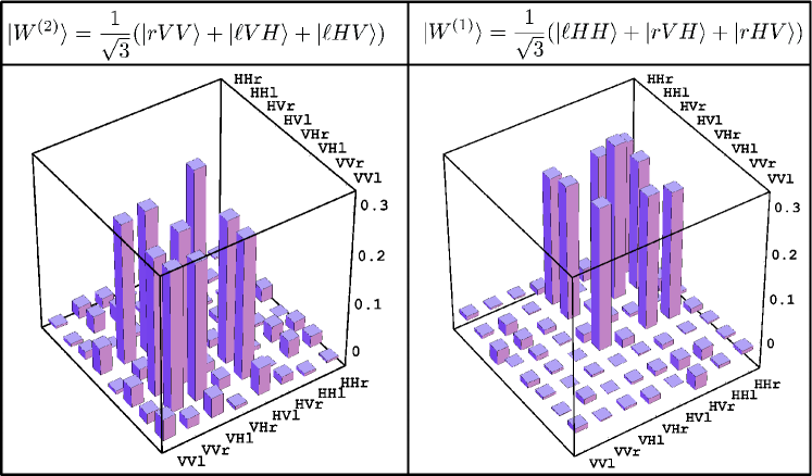
Figure 2: Tomographically reconstructed density matrix (real part) of $|W^{(2)}\rangle_{abc}$ (left) and $|W^{(1)}\rangle_{abc}$ (right) obtained by the procedure described in the text. The contributions of the imaginary part are negligible. We have a state fidelity with the target states ${\cal F}=\langle W^{(p)}|\varrho_{p}|W^{(p)}\rangle\simeq 0.87$, consistently for $p=1,2$.

We then performed the tomographic reconstruction of the density matrices $\varrho_{1,2}$ describing the states of the remaining three (polarization and momentum) qubits by projecting each of them onto the elements of a (statistically complete) subset of 64 states extracted from the 216 ones obtained by taking the tensor products of $\{|H\rangle,|V\rangle,|\pm_{x}\rangle,|\pm_{y}\rangle\}$ with $|+_{k}\rangle$ ($|-_{k}\rangle$) the eigenstates of the $k$-Pauli matrix ($k=x,y$) with eigenvalue $+1$ (-1). The two qubits encoded in the polarization DOF were projected onto the necessary elements by using a usual analysis setup before each detector, composed by a quarter-waveplate, a half-waveplate and a polarizing beam splitter. The momentum encoded qubit was measured by exploiting the second passage through the BS which allows to project onto the eigenstates of the necessary Pauli operators. The results of the tomographic analysis are shown in Fig. 2, where we also report the value of the state fidelity ${\cal F}=\langle W^{(p)}|\varrho_{p}|W^{(p)}\rangle=(0.87\pm 0.01)$, consistently for the two projected states.

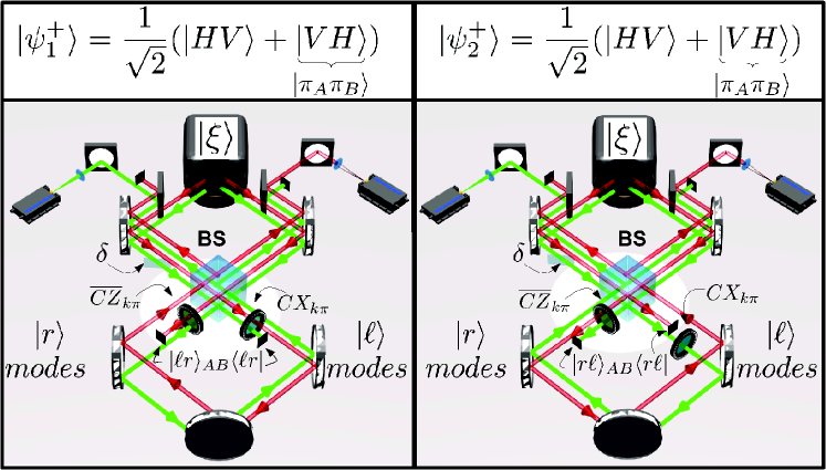
Figure 3: Experimental setup used for generation and analysis of the two-qubit $|\psi^{+}_{1,2}\rangle$ states obtained from the projection of the momentum qubits $c,d$ of the quadripartite Dicke state $|D^{(2)}_{4}\rangle$ onto $|\ell r\rangle_{AB}$ (left) and $|r\ell\rangle_{AB}$ (right), respectively. The red (green) modes represent the optical path followed by photon A(B).

Our study of the inherent entanglement sharing structure within $|D^{(2)}_{4}\rangle$ continues with a further projection. Indeed, by following the same procedure of Eq. (4), one finds

$$|D^{(2)}_{4}\rangle=\frac{1}{\sqrt{6}}(|0011\rangle_{abcd}+|1100\rangle_{abcd})+\sqrt{\frac{2}{3}}|\psi_{+}\rangle_{ab}|\psi_{+}\rangle_{cd}$$ (5)

where we have introduced the Bell state $|\psi^{+}\rangle{=}(|01\rangle{+}|10\rangle)/\sqrt{2}$. Therefore, by projecting the quadripartite Dicke state onto $|01\rangle_{cd}$ or $|10\rangle_{cd}$, we are able to obtain the reduced two-qubit register prepared in $|\psi^{+}\rangle_{ab}$. We have experimentally verified that this is indeed the case by projecting the Dicke state created by our state-generation process onto $|10\rangle_{cd}$ and $|01\rangle_{cd}$ and performing a two-qubit QST on the rest of the register. Here the necessary projections were performed by suitably selecting the modes emerging from the BS. In the previous case we needed to select only one mode since we projected only qubit $d$. In order to project also qubit $c$ we had to select an optical mode emerging from the BS also for photon A.

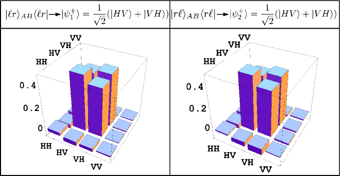
Figure 4: Tomographically reconstructed density matrices of $|\psi^{+}_{1,2}\rangle_{ab}$ achieved by projecting $|D^{(2)}_{4}\rangle$ onto $|10\rangle_{cd}$ ($|\ell r\rangle_{AB}$, left) and $|01\rangle_{cd}$ ($|r\ell\rangle_{AB}$, right), respectively. We show the real part of the elements of each density matrix, the imaginary parts being negligible. The fidelities, obtained with respect to the theoretical state, are $\mathcal{F}_{|\psi^{+}_{1}\rangle}=0.92\pm 0.07$ and $\mathcal{F}_{|\psi^{+}_{2}\rangle}=0.92\pm 0.06$.

The results of such analysis are given in Fig. 4, where we have distinguished the reduced states achieved by projecting onto $|10\rangle_{cd}$ or $|01\rangle_{cd}$ by labeling them as $|\psi^{+}_{1}\rangle$ or $|\psi^{+}_{2}\rangle$, respectively (needless to say, ideally there should be no difference between them). The associated state fidelity $\geq 90\%$, independently of the projection, thus demonstrating the quality of the reduced two-qubit states.

We conclude this part of our study by describing the results of a further reduction performed on the initial four-qubit Dicke resource. We thus implement the projection onto three qubits of the register. We already discussed how the projections onto $|01\rangle_{cd}$ or $|10\rangle_{cd}$ were implemented. The last reduction was implemented by selecting the state $|1\rangle_{a(b)}$ and performing the QST on the qubit $b(a)$. It is worth reminding that qubits $a$ and $b$ were encoded in the polarization DOF, so the projection of these qubits could be performed by selecting the physical state $|V\rangle$ before the detector. In Fig. 5 we show the results of the projections onto the states $|101\rangle_{acd}$, $|110\rangle_{acd}$, $|101\rangle_{bcd}$, $|110\rangle_{bcd}$. Needless to say, the increasing quality of the reduced states is due to the decreasing size of the computational register, which makes state characterisation much more agile, and the filtering effects of the projective measurements [24].

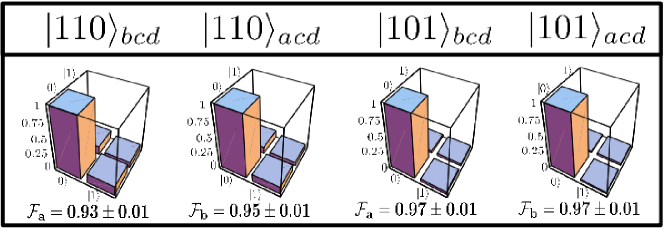
Figure 5: Tomographically reconstructed density matrices by projecting three qubits of the Dicke states onto the shown states. The fidelities have been calculated with respect to the expected theoretical states. We show the real part of the elements of each density matrix, the imaginary parts being negligible.

3 Quantum and classical correlations in a tripartite system

The good quality of the tripartite state produced through the projection above described allows us to go beyond the mere reconstruction of the density matrix of the system. In particular, in what follows we concentrate on an analysis of the trade-off between quantum and classical correlations in a multi-qubit state, a topic that is currently enjoying a strong and extensive attention by the community interested in quantum information processing [29]. In the remainder of the paper we thus consider the KW relation [28] and apply it to the experimental $|W^{(1)}\rangle$ state. In order to provide a self-contained account of our goal, in what follows we briefly introduce the KW relation and identify its context of relevance.

3.1 The KW relation

Quantum correlations beyond entanglement have been the centre of an extensive quest for the understanding of their significance, relevance and use in the panorama of quantum-empowered information processing and for the study of non-classicality [29]. Such investigation passes through the ab initio definition of quantum correlations [30, 31, 32, 33, 34], their evaluation for different classes of systems [33, 35], and their operational interpretation given in terms of the role that they have in quantum communication protocols [36, 37, 38, 39, 40]. In this context, in Ref. [28] the KW relation was introduced to capture the trade-off between entanglement and classical correlations in a pure tripartite system. This has been recently used as the stepping-stone for various results, such as conservation laws and the formulation of a chain-rule for discord [41, 42].

The KW relation is based, in some sense, on the monogamous nature of entanglement: if a system $\alpha$ is correlated with both $\beta$ and $\gamma$, it cannot be maximally correlated with any of them [43]. The KW relation shows that the degree of correlations that, say, $\beta$ can share with the other two is limited by its von Neumann entropy. In more quantitative terms and considering only pure tripartite states for the moment, the KW relation reads

$$J(\beta|\alpha)+E(\beta,\gamma)=S(\beta),$$ (6)

where any permutation of the systems’ indices will lead to similar equalities. Here, $E(\beta,\gamma)$ is the entanglement of formation shared by $\beta$ and $\gamma$ [44], $S(B)=-\mathrm{Tr}[\rho_{\beta}\log_{2}(\rho_{\beta})]$ is the von Neumann entropy of $\beta$ only and $J(\beta|\alpha)\equiv\max_{{\cal E}_{\alpha}}J(\beta|\{{\cal E}_{\alpha}\})$ measures the amount of classical correlations within the state of systems $\alpha$ and $\beta$ upon the performance of a measurement (described by the positive-operator-valued-measurement $\{{\cal E}_{\alpha}\}$) over $\alpha$. Here, $J(\beta|\{{\cal E}_{\alpha}\})=S(\beta)-S(\beta|{\cal E}_{\alpha})$, with $S(\beta|{\cal E}_{\alpha})$ the quantum conditional entropy of the state of system $\beta$ [45]. The maximization inherent in the definition of $J(\beta|\alpha)$ is necessary to remove any dependence on the specific choice of $\{{\cal E}_{\alpha}\}$. Moreover, it was shown in [47] that orthogonal projective measurements are optimal for rank-2 states and provide a very tight bound for rank 3 and 4, therefore the maximisation can be performed within this class of measurements.

As mentioned above, by permuting the systems’ labels, we find five more analogous KW relations. Notice that the relations are six because classical correlations are asymmetrical by definition (as one needs to specify the part the measurement is carried on). If the tripartite state is mixed, the left-hand side of Eq. (6) is always upper-bounded by the right-hand side. In the remainder of this paper we use the quantity defined as the difference between the right and left-hand side of Eq. (6), that is

$$KW=S(\beta)-J(\beta|\alpha)-E(\beta,\gamma).$$ (7)

Needless to say, the value achieved by a pure state is zero.

3.2 Experimental investigation of the KW relation

The maximization necessary for the evaluation of the amount of classical correlations makes the explicit evaluation of the KW relation difficult, in general. However, for the particular case of our experimental investigation, state symmetries come to our aids. Indeed, the three-qubit reduced states $\varrho_{1,2}$ that we have achieved starting from $|D^{(2)}_{4}\rangle$ has a large overlap with the ideal $|W^{(1,2)}\rangle$. We can thus exploit the symmetries inherent in the latter to derive a manageable expression for the KW relation evaluated over the experiment state. Needless to say, we will have the caveat of dealing with the KW inequality rather than Eq. (6). In order to fix the ideas, we will consider the subspace of the three-qubit Hilbert space spanned by $\{|001\rangle,|010\rangle,|100\rangle\}$, so that our results will be valid for $|W^{(1)}\rangle$ (although similar conclusions can be drawn for $|W^{(2)}\rangle$). We start evaluating the quantities entering Eq. (7) for a state of systems $\alpha,\beta$ and $\gamma$ of the following form

$$\sigma{=}\left(\begin{array}[]{cccccccc}0&0&0&0&0&0&0&0\!\!\!\\ 0&p&c&0&c&0&0&0\!\!\!\\ 0&c&p&0&c&0&0&0\!\!\!\\ 0&0&0&0&0&0&0&0\!\!\!\\ 0&c&c&0&p&0&0&0\!\!\!\\ 0&0&0&0&0&0&0&0\!\!\!\\ 0&0&0&0&0&0&0&0\!\!\!\\ 0&0&0&0&0&0&0&0\!\!\!\\ \end{array}\right),$$ (8)

where we deliberately keep all the quantities symbolic so as to have an expression that depends explicitly on the populations of the state $|001\rangle$, $|010\rangle$, and $|100\rangle$ and on the respective coherences. We get

$$S(\beta) = -p(2+3\log_{2}{p}),$$

$$E(\beta,\gamma) = -\frac{1}{2}(1+\sqrt{1-4p^{2}})\log_{2}\left[{\frac{1}{2}(1+\sqrt{1-4p^{2}}})\right]$$

$$- \frac{1}{2}(1-\sqrt{1-4p^{2}})\log_{2}\left[{\frac{1}{2}(1-\sqrt{1-4p^{2}}})\right],$$

$$J(B|A) = -p\log_{2}{p}-2p\log_{2}{2p}$$ (9)

$$+ \frac{1}{2p}\left\{(3p^{2}-\sqrt{4c^{2}p^{2}+p^{4}})\log_{2}\left[{\frac{1}{2}\left(1-\frac{\sqrt{4c^{2}p^{2}+p^{4}}}{3p^{2}}\right)}\right]\right.$$

$$+ \left.(3p^{2}+\sqrt{4c^{2}p^{2}+p^{4}})\log_{2}\left[{\frac{1}{2}\left(1+\frac{\sqrt{4c^{2}p^{2}+p^{4}}}{3p^{2}}\right)}\right]\right\}.$$

The amount of classical correlations were calculated by maximisation over the complete set of orthogonal projectors given by $\Pi_{j}=|\theta_{j}\rangle\left\langle\theta_{j}\right|$ with $j=1,2$, $|\theta_{1}\rangle=\cos{\theta}|0\rangle+e^{\imath\phi}\sin{\theta}|1\rangle$ and $|\theta_{2}\rangle=e^{-\imath\phi}\sin{\theta}|0\rangle-\cos{\theta}|1\rangle$. For the specific state chosen it turns out that the maximisation does not depend on the $\phi$ parameter and is achieved for $\theta=\pi/4$. Taking an experimental viewpoint, we notice that the populations $p$ and coherences $c$ can be written explicitly as function of the following correlators (calculated over the state of the three-particle system)

Table 1: Table of the correlators needed in order to evaluate the KW relation for symmetric three-qubit states leaving in the single-excitation subspace. The experimental values are reported with their associated uncertainties determined by associating Poissonian fluctuations to the coincidence counts needed to reconstruct each correlator.

Correlator	Value
$Z_{a}Z_{b}Z_{c}$	$0.87\pm 0.02$
$Z_{a}Z_{b}I_{c}$	$0.35\pm 0.04$
$Z_{a}I_{b}I_{c}$	$0.26\pm 0.04$
$X_{a}X_{b}Z_{c}$	$0.55\pm 0.04$
$Y_{a}Y_{b}Z_{c}$	$0.70\pm 0.03$
$X_{a}X_{b}I_{c}$	$0.66\pm 0.03$
$Y_{a}Y_{b}I_{c}$	$0.52\pm 0.04$

$$p=[-\langle Z_{\alpha}Z_{\beta}Z_{\gamma}\rangle+\langle I_{\alpha}I_{\beta}I_{\gamma}\rangle-P(\langle Z_{\alpha}Z_{\beta}I_{\gamma}\rangle)/3+P(\langle Z_{\alpha}I_{\beta}I_{\gamma}\rangle)]/8,$$

$$c=[P(\langle X_{\alpha}X_{\beta}Z_{\gamma}\rangle)+P(\langle Y_{\alpha}Y_{\beta}Z_{\gamma}\rangle)+P(\langle X_{\alpha}X_{\beta}I_{\gamma}\rangle)+P(\langle Y_{\alpha}Y_{\beta}I_{\gamma}\rangle)]/24,$$

where $P(\cdot)$ performs the sum of the permutation over $\alpha$, $\beta$ and $\gamma$ of its argument. With this at hand, it is now clear that the KW relation can be evaluated by means of only eight correlators. In turn, the latter could be reconstructed experimentally starting from only five measurement settings [48]. Interestingly, due to the state symmetries, such correlators are exactly those needed to evaluate the fidelity-based entanglement witness for $|W^{(1)}\rangle$, when optimally decomposed into local measurement settings [48]. As such, a single set of local measurements would allow for the determination of the genuine tripartite entangled nature of our projected state [27] and the analysis of the sharing of correlations among its constituents. In the specific case of our experimental implementation, though, a decomposition into the seven inequivalent settings that can be identified in Eq. (3.2) was more convenient and has thus been used.

When applied to the experimental state $\varrho_{1}$, whose experimentally reconstructed correlators are given in Table 1, with the associations $\alpha=a,\beta=b$ and $\gamma=c$, the combination of the expressions in Eqs. (3.2) gives us the value $KW=0.04\pm 0.02$, which is very close to the value expected for $|W^{(1)}\rangle$. Needless to say, this result should be considered as a lower bound to the actual value that Eq. (7) would take over an experimentally generated state, in particular due to the lack of perfect symmetries which played an important role in the determination of the expressions in Eqs. (3.2). This is, again, fully in line with similar issues affecting the evaluation of entanglement witnesses over experimental states that do not fulfill the expected degree of symmetry that characterise ideal states. Indeed, the evaluation of Eq. (7) over the tomographically reconstructed state returns a value (averaged over the various permutations of systems’ indices) of $0.36\pm 0.04$, which is significantly different from the value estimated above based on only 8 correlators and the underlying symmetry assumptions. The argument above can be made more quantitative by noticing that, while the numerical functions $J(a|\{\Pi_{b}\})$ and $J(b|\{\Pi_{a}\})$ evaluated over $\varrho_{1}$ are almost independent of $\phi$ and reach their maximum for $\theta$ close to $\pi/4$, the same does not apply for classical correlation involving the $c$ qubit, thus witnessing the asymmetry of the experimental state. This can be ascribed to the fact that qubit $c$ is physically encoded in the momentum DOF of a light mode, differently from $a$ and $b$, which are both encoded in polarization.

While we are currently working on a formulation that could encompass possible asymmetries in the tested state yet retaining the handiness of an expression that could be experimentally determined by only a handful of measurement settings, we mention that a model that is in better agreement with the experimental values of the KW would involve a mixture of $|W^{(1)}\rangle$ with a fully mixed state of three qubits. This model is motivated by considering that, experimentally, such projected three-qubit state was created by performing a measurement over a quadripartite having a non-ideal estimated fidelity greater than $78\%$ with the ideal Dicke resource and that, for all practical purposes, can be rightly written as $\rho_{Dicke}=p(|{D^{(2)}_{4}}\rangle\langle{D^{(2)}_{4}}|)+\frac{1-p}{16}I_{16}$ [25, 27], where the statistical mixture parameter most compatible with the above mentioned fidelity is $p=0.765\pm 0.005$. It is straightforward to check that such a model provides a value of Eq. (7) equal to $0.25\pm 0.01$, that is significantly closer to the actual experimental value, still using only eight correlators overall. By generalising this model to anisotropic noise added to an ideal $|W^{(1)}\rangle$ state, we will be able to come up with a broadly applicable expression for the handy experimental estimate of the expectation value of Eq. (7). Such analysis goes beyond the scopes of this work and will be presented elsewhere [49].

4 Conclusions

We have explored the correlation properties of states obtained by projecting out part of a quadripartite system prepared in a symmetric Dicke state with two excitations and encoded in a high quality photonic hyperentangled state. By designing properly the projections to perform, we have obtained reduced three, two and one-qubit states very close to the expected ones, as shown by the fidelity between the ideal reduced resources and the tomographically reconstructed density matrices of the experimental states. The good quality of the three-qubit Dicke states with one and two excitations obtained in our experiment has paved the way to the experimental verification of a simplified expression for the monogamy of correlations in a tripartite state embodied by the celebrated KW relation [28]. We have highlighted both the advantages, in terms of the very small number of experimental correlators needed for the reconstruction of the expression that we have formulated, and the limitations of our approach, which is heavily based on the symmetries of the ideal state at hand. Our work inspires an experimentally friendly exploration of the correlation properties of multipartite qubit states in state-of-the-art photonic settings characterized by high reconfigurability, exquisite control, and reliable tomographic tools for state diagnostics.

References

References

- [1] P. Kok, W. J. Munro, K. Nemoto, T. C. Ralph, J. Dowling, and G. J. Milburn, Rev. Mod. Phys. 79, 135 (2007).
- [2] J.-W. Pan, Z.-B. Chen, C.-Y. Lu, H. Weinfurter, A. Zeilinger, and M. Zukowski, Rev. Mod. Phys. 84, 777 (2012).
- [3] D. Bouwmeester et al., Nature 390, 575 (1997).
- [4] D. Boschi et al., Phys. Rev. Lett. 80, 1121 (1998).
- [5] M. Riebe et al., Nature 429, 734 (2004).
- [6] P. Walther, et al. Nature 434, 169 (2005); M. S. Tame, R. Prevedel, M. Paternostro, P. Bohi, M. S. Kim, and A. Zeilinger, Phys. Rev. Lett. 98, 140501 (2007); R. Prevedel, et al., Phys. Rev. Lett. 99, 250503 (2007); W.-B. Gao, et al. Phys. Rev. Lett. 104, 020501 (2010); G. Vallone, E. Pomarico, F. De Martini, and P. Mataloni, Phys. Rev. Lett. 100, 160502 (2008); G. Vallone, G. Donati, R. Ceccarelli, and P. Mataloni, Phys. Rev. A 81, 052301 (2010); R. Prevedel, et al., Nature 445, 65 (2007); G. Vallone, G. Donati, N. Bruno, A. Chiuri, and P. Mataloni, Phys. Rev. A 81, 050302(R) (2010).
- [7] Z. Zhao, et al., Nature 430, 54 (2004).
- [8] X.-S. Ma, B. Dakic, W. Naylor, A. Zeilinger, and P. Walther, Nature Phys. 7, 399 (2011); X.-S. Ma, et al. arXiv:1205.2801 (2012).
- [9] L. Sansoni, et al., Phys. rev. Lett. 108, 010502 (2012); A. Peruzzo, et al., Science 329, 1500 (2010).
- [10] R. Prevedel, A. Stefanov, P. Walther, and A. Zeilinger, New J. Phys. 9, 205 (2007); M. Paternostro, M. S. Tame, and M. S. Kim, New J. Phys. 7, 226 (2005).
- [11] B. P. Lanyon, et al. Nature Chem. 2, 106 (2009).
- [12] A. Aspuru-Guzik, and P. Walther, Nature Phys. 8, 285 (2012).
- [13] F. L. Semiao, and M. Paternostro, Quant. Inf. Proc. 11, 67 (2011).
- [14] D. F. V. James, et al., Phys. Rev. A 64, 052312 (2001).
- [15] M. A. Nielsen and I. L. Chuang, Quantum Computation and Quantum Information (Cambridge University Press, 2000).
- [16] A. Chiuri, G. Vallone, M. Paternostro, and P. Mataloni, Phys. Rev. A 84, 020304(R) (2011).
- [17] H. Ollivier, and W. H. Zurek, Phys. Rev. Lett. 88, 017901 (2001).
- [18] L. Henderson, and V. Vedral, J. Phys. A: Math. Theor. 34, 6899 (2001).
- [19] B. Dakic, V. Vedral, and C. Brukner, Phys. Rev. Lett. 105, 190502 (2010).
- [20] B. Dakic, et al., arXiv:1203.1629 (2012).
- [21] R. Auccaise, J. Maziero, L. C. Celeri, D. O. Soares-Pinto, E. R. deAzevedo, T. J. Bonagamba, R. S. Sarthour, I. S. Oliveira, and R. M. Serra, Phys. Rev. Lett. 107, 070501 (2011); M. Gu, H. M. Chrzanowski, S. M. Assad, T. Symul, K. Modi, T. C. Ralph, V. Vedral, and P. K. Lam, arXiv:1203.0011 (2012); R. Blandino, M. G. Genoni, J. Etesse, M. Barbieri, M. G. A. Paris, P. Grangier, and R. Tualle-Brouri, ArXiv:1203.1127 (2012)
- [22] X.-C. Yao, et al., Nature Photon. 6, 225 (2012).
- [23] R. Ceccarelli, G. Vallone, F. De Martini, P. Mataloni, and A. Cabello, Phys. Rev. Lett. 103, 160401 (2009).
- [24] R. Prevedel, et al., Phys. Rev. Lett. 103, 020503 (2009); W. Wieczorek, et al., Phys. Rev. Lett. 103, 020504 (2009).
- [25] A. Chiuri, G. Vallone, N. Bruno, C. Macchiavello, D. Bruß, and P. Mataloni, Phys. Rev. Lett. 105, 250501 (2010).
- [26] A. Chiuri, C. Greganti, and P. Mataloni, Eur. Phys. J. D (to appear, 2012).
- [27] A. Chiuri, C. Greganti, M. Paternostro, G. Vallone, and P. Mataloni, arXiv:1112.5307 (2011).
- [28] M. Koashi, and A. Winter, Phys. Rev. A 69, 022309 (2004).
- [29] K. Modi, A. Brodutch, H. Cable, T. Paterek, and V. Vedral, arXiv:1112.6238 (2011).
- [30] J. Oppenheim, M. Horodecki, P. Horodecki, and R. Horodecki, Phys. Rev. Lett. 89, 180402 (2002).
- [31] W. H. Zurek, Phys. Rev. A 67, 012320 (2003).
- [32] B. Groisman, S. Popescu, and A. Winter, Phys. Rev. A 72, 032317 (2005).
- [33] S. Luo, Phys. Rev. A 77, 022301 (2008).
- [34] K. Modi, et al., Phys. Rev. Lett. 104, 080501 (2010).
- [35] B. Bylicka and D. Chruscinski, Phys Rev A 81, 062102 (2010).
- [36] A. Datta, A. Shaji, and C. M. Caves, Phys. Rev. Lett. 100, 050502 (2008).
- [37] D. Cavalcanti, et al., Phys. Rev. A 83, 032324 (2011).
- [38] M. Piani, et al., Phys. Rev. Lett. 106, 220403 (2011); A. Streltsov, H. Kampermann, and D. Bruß, Phys. Rev. Lett. 106, 160401 (2011).
- [39] L. Mazzola and M. Paternostro, Nature Sci. Rep. 1, 199 (2011).
- [40] T. K. Chuan, et al. arXiv:1203.1268 (2012); A. Streltsov, H. Kampermann, and D. Bruß, arXiv:1203.1264 (2012).
- [41] F. F. Fanchini, M. F. Cornelio, de M. C. Oliveira, and A. O. Caldeira, Phys. Rev. A 84, 012313 (2011).
- [42] F. F. Fanchini, L. K. Castelano, M. F. Cornelio, and M. C. de Oliveira, New J. Phys. 14, 013027 (2012).
- [43] V. Coffman, J. Kundu, and W. K. Wootters, Phys. Rev. A 61, 052306 (2000)
- [44] For two qubits, the entanglement of formation is given by [46] , with and being the concurrence. Here, is the set of eigenvalues (arranged in non-increasing order) of the Hermitian matrix where and is the complex conjugate of the density matrix.
- [45] Given with elements ( being a measurement operator), the joint state is transformed into . Each measurement outcome occurs with a probability and collapses into the post-measurement conditional state . The quantum conditional entropy is thus defined as .
- [46] C. H. Bennett, D. P. DiVincenzo, J. A. Smolin, and W. K. Wootters, Phys. Rev. A 54, 3824 (1996); W. K. Wootters, Phys. Rev. Lett. 80, 2245 (1998).
- [47] F. Galve, G. Giorgi, and R. Zambrini, EPL 96, 40005 (2011).
- [48] O. Gühne and P. Hyllus, Int. J. Theor. Phys. 42, 1001 (2003).
- [49] L. Mazzola, et al. (to appear, 2012).