Longitudinal waves in electrically polarized quantum Fermi gas: quantum hydrodynamics approximation

Abstract

The method of many-particle quantum hydrodynamics has been recently developed, particularly this method has been used for an electrically polarized Bose-Einstein condensate. In this paper, we present the development of this method for an electrically polarized three dimensional Fermi gas. We derive corresponding dynamical equations: equation polarization and equation of polarization current evolution as well as the Euler and continuity equations. We study dispersion dependencies of collective excitations in a polarized Fermi gas and consider interference of an equilibrium polarization on dispersion properties.

I I. Introduction

Electrically polarized ultracold Fermi gases have been in the center of attention  Baranov arxiv 07 review along with the electrically polarized Bose-Einstein condensate  Baranov arxiv 07 review - Ni PCCP 09 . It is well-known that generalization of the Gross-Pitaevskii equation has been used for description of the electrically polarized Bose-Einstein condensate what was suggested in Ref.s  Yi PRA 00 - Santos PRL 00 . An analogous non-linear Schrodinger equation can be used for study of electrically polarized Fermi gases. However, using of the kinetic equation is more prevailing (see for example  Sogo NJP 09 ,  Zhang PRA 09 ,  Zhang PRA 11 ). In simple cases the set of quantum hydrodynamics (QHD) equations is equivalent to corresponding non-linear Schrodinger equation  Andreev PRA08 , but it we are interested in studying of evolution of electrical dipole moment direction we need more general equation set. Such equations can be derived by means of the QHD method, which allows to get equation of polarization evolution, as it was demonstrated for electrically polarized Bose-Einstein condensate  Andreev arxiv Pol - Andreev arxiv 12 transv dip BEC . This paper is dedicated to both the development of the method of many-particle QHD for electrically polarized ultracold Fermi gas and studying of dispersion of bulk collective excitations inwhere.

To be certain we will consider fermions with the spin 1/2. We interesting in dynamic of electric polarization, and it’s influence on static and dynamic properties of the ultracold fermions. We do not consider the dynamic of spin of atoms, for simplicity. However, at consideration of nonlinear properties of the electrically polarized ultracold fermions the role of a spin could be important. The nonlinear Schrodinger equation is usually used for quantum gases studying, so it is important to discuss limits of validity of such approximation. In the case of the electrically polarized quantum gases, in the corresponding non-linear Schrodinger equation a new term is added. However, this approximation includes interaction among parallel dipoles and influence of this interaction on particles translational motion (see Fig.1), and does not account spatial and temporal evolution of dipoles direction pictured on Fig.2. In Ref.  Andreev arxiv Pol authors developed method accounted spatially inhomogeneous distribution of dipoles directions and it’s temporal evolution. This method includes the potential of interaction unparallel dipoles, and it also includes additional equations determining evolution of dipoles moment of a volume unit. It was based on the method of many-particle QHD. In our previous papers  Andreev arxiv Pol -  Andreev PRB11 we developed the method of the many-particle QHD for the electrically polarized BEC. This approximation allows to describe as the spatial and the temporal evolution of the electric dipole moments including evolution of it’s directions. Evolution of dipoles direction gives influence on translational motion of particles due to tensor nature of the dipole-dipole interaction. Equations of the QHD are derived directly from the many-particle Schrodinger equation. QHD description of unpolarized ultracold fermions was presented in Ref.s  Andreev PRA08 and  Zezyulin arxiv 12 .

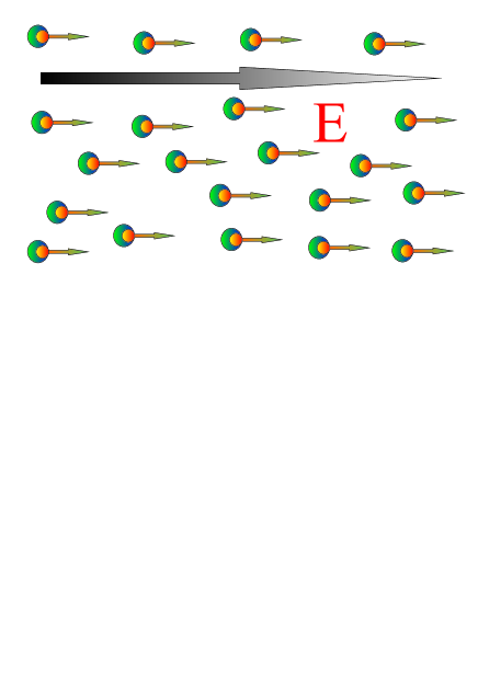
Figure 1: (Color online) The figure describes the picture of ultracold Fermi particles having electric dipole moment and obeying to the generalization of the non-linear Schrodinger equation (the analog of the Gross-Pitaevskii equation which used for polarized Bose-Einstein condensate description). This figure presents system of particles with parallel electric dipole moment. Arrow by the circle imitates particle dipole and it’s direction.

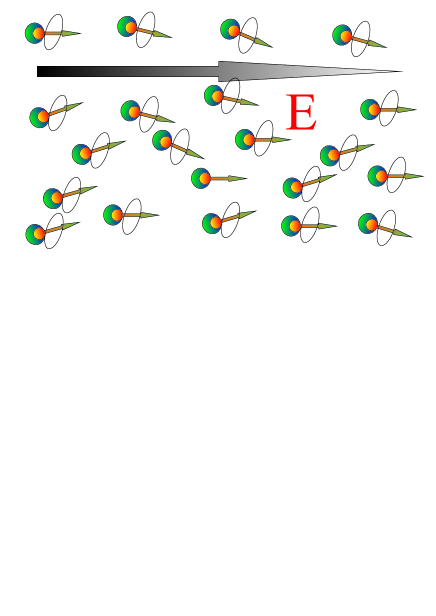
Figure 2: (Color online) The figure presents the picture of particles having electric dipole moment where direction of electric dipole moments evaluate in time (rotating or oscillating) and have different directions in different points of space (it might be caused by difference of phase at rotation). Arrow by the circle imitates particle dipole and it’s direction. Round lines around arrow minds rotation of dipoles.

At studying of ultracold electrically polarized Fermi gas, many researchers actually prefer using the kinetic equation  Sogo NJP 09 ,  Zhang PRA 09 ,  Zhang PRA 11 , which describes evolution of the distribution function $f(\textbf{r},\textbf{p},t)$ defined in the six dimensional space of coordinate $r$ and momentum $p$. The kinetic equation allows us to get a set of hydrodynamics equations for evolution of the particle concentration $n(\textbf{r},t)=\int f(\textbf{r},\textbf{p},t)d\textbf{p}$, momentum density $\textbf{j}(\textbf{r},t)=\int\textbf{p}f(\textbf{r},\textbf{p},t)d\textbf{p}$, energy and higher moments of the distribution function. However the usually used kinetic equation corresponds to the hydrodynamic equations, which do not include the equations of polarization evolution, and, so it describe polarization evolution caused by changing of particles concentration only. We believe that such approximation might be enough for getting description of collective excitation of the sample shape, but it is not enough for bulk waves description in the electrically polarized Fermi gas.

In Ref.s  Sogo NJP 09 ,  Zhang PRA 09 the kinetic equation was derived via the Wigner function with parallel dipoles without dynamics of electric dipoles direction. In Ref.  Zhang PRA 11 this equation has been used for dynamics of the dipolar Fermi gas at finite temperature. The functional renormalization group technique used in Ref.  Bhongale PRL 12 to get the zerotemperature phase diagram of dipolar fermions on a two-dimensional square lattice at half filling for the system of dipoles pointing in the same direction.

A. R. P. Lima and A. Pelster  Lima PRA 10 presented the derivation of the continuity and Euler equations for dipoles fermions considering the evolution of the one-body density matrix  Bruun PRL 99 - Ring book 04 . They considered the set of equations which is equivalents to the corresponding non-linear Schrodinger equation and describes dynamics of parallel dipoles. In QHD description these equations are only a part of the set of QHD equations. Here we present more general set of QHD equations which fully described dynamics of electrical polarization in polarized Fermi gas. The Habbard’s model is also very useful  Lu 11 arxiv ,  Gadsbolle 11 arxiv , but we are not going to discuss it here.

The set of the many-particle QHD equations obtained in Ref.s  Andreev arxiv Pol -  Andreev RPJ 12 contains four equation, which are the continuity equation, the Euler equation (the momentum balance equation), the equation of polarization evolution and the equation of polarization current evolution. These equations appear along with the equations of field, which are $\nabla\textbf{E}=-4\pi\nabla\textbf{P}$ and $\nabla\times\textbf{E}=0$, where E is the electric field, and P is the density of electric dipole moment, they are a pair of the Maxwell’s equations. This model give us possibility to study the evolution of polarization, and it’s influence on particle motion. It was found that in linear approximation where are two wave solution instead of the Bogoliubov’s mode existing in the unpolarized Bose-Einstein condensate.

In this paper we develop the many-particles QHD for the electrically polarized ultracold fermions. We derive corresponding the continuity equation, the Euler equation, the equation of polarization evolution and the equation of polarization current evolution. Expecting to obtain two wave solutions instead of one existing in the unpolarized ultracold Fermi gas we consider linear approximation of the QHD equations.

This paper is organized as follows. In Sec. II we present the derived set of the QHD equations for the electrically polarized ultracold fermions. In Sec. III we describe the method used for the solving of the QHD equations and present formula for dispersion dependence of waves in the system of the electrically polarized ultracold fermions. In Sec. IV we present numerical analysis of the dispersion dependence. In Sec. V we present the brief summary of our results.

II II. Basic equations

Here we will briefly present the set of the QHD equations for the electrically polarized ultracold Fermi gas. The method of theirs derivation described in Ref.s  Andreev arxiv 12 (2) and  Andreev PRB11 . It was done for the Bose-Einstein condensate, but the method of derivation is the same, this is why we do not present details of derivation and present resulting equations only.

The first equation of the QHD equations system is the continuity equation

$$\partial_{t}n+\partial^{\alpha}(nv^{\alpha})=0,$$ (1)

where $n$ is the particles concentration and $v^{\alpha}$ is the velocity field.

The momentum balance equation for the polarized ultracold fermions has the form

$$mn(\partial_{t}+\textbf{v}\nabla)v^{\alpha}+\frac{\hbar^{2}}{5m}(3\pi^{2})^{\frac{2}{3}}\partial^{\alpha}n^{\frac{5}{3}}$$

$$-\frac{\hbar^{2}}{4m}\partial^{\alpha}\triangle n+\frac{\hbar^{2}}{4m}\partial^{\beta}\Biggl{(}\frac{\partial^{\alpha}n\cdot\partial^{\beta}n}{n}\Biggr{)}$$

$$=-\Upsilon_{2}(\partial^{\alpha}n)\triangle n-2\Upsilon_{2}(\partial^{\alpha}\partial^{\beta}n)\partial_{\beta}n$$

$$+3\Upsilon_{2}n\partial^{\alpha}\triangle n-4(3\pi^{2})^{\frac{2}{3}}\Upsilon_{2}\partial^{\alpha}n^{\frac{8}{3}}+P^{\beta}\partial^{\alpha}E^{\beta},$$ (2)

where

$$\Upsilon_{2}\equiv\frac{\pi}{30}\int dr(r)^{5}\frac{\partial U(r)}{\partial r}.$$ (3)

In equation (2) we defined a parameter $\Upsilon_{2}$ as (3). This definition differs from the one in Ref.s  Andreev PRA08 ,  Zezyulin arxiv 12 . In left-hand side of equation we have three terms proportional to $\hbar^{2}$, first of them is the gradient of the Fermi pressure. Other two are the quantum Bohm potential, they appear as a result of using of the quantum kinematics. The first four terms in the right-hand side of equation (2) describe the short range interaction in the system of ultracold fermions appearing in the third order by the interaction radius. They occur because of taking into account of the SRI potential $U_{ij}$. The interaction potential $U_{ij}$ defines the macroscopic interaction constant $\Upsilon_{2}$. The first three terms in the right-hand side of equation contain high space derivatives of particle concentration and, thus, have something common with the quantum Bohm potential. The fourth term arises because of the dependence of the interaction on the Fermi pressure. Therefore the Fermi pressure gives contribution in two terms, kinetic and dynamical. The last term in the equation (2) describes force field which affects the dipole moments in a unit of volume as the effect of the external electrical field and the field produced by other dipoles. The last term is written using the self-consistent field approximation  Andreev PRB11 .

We have also field equations

$$\nabla\textbf{E}(\textbf{r},t)=-4\pi\nabla\textbf{P}(\textbf{r},t),$$ (4)

and

$$\nabla\times\textbf{E}(\textbf{r},t)=0.$$ (5)

Equations (4) and (5) allow us to consider longitudinal waves only, i.e. electric field of wave parallel to the direction of propagation.

In the case particles does not contain the dipole moment, the continuity equation and the momentum balance equation form a closed system of equations. When the dipole moment is taken into account in a momentum balance equation, a new physical value emerges, a polarization vector field $P^{\alpha}(\textbf{r},t)$. This causes system of equations to become incomplete.

We need next equation for investigation of the dispersion of the collective excitations is the equation of polarization evolution

$$\partial_{t}P^{\alpha}+\partial^{\beta}R^{\alpha\beta}=0,$$ (6)

$R^{\alpha\beta}(\textbf{r},t)$ is the current of polarization.

The equation (6) does not contain information about the effect of the interaction on the polarization evolution. The evolution equation of $R^{\alpha\beta}(\textbf{r},t)$ can be constructed by analogy with the above derived equations. Using a self-consistent field approximation of the dipole-dipole interaction we obtain an equation for the polarization current $R^{\alpha\beta}(\textbf{r},t)$ evolution

$$\partial_{t}R^{\alpha\beta}+\partial^{\gamma}\biggl{(}R^{\alpha\beta}v^{\gamma}+R^{\alpha\gamma}v^{\beta}-P^{\alpha}v^{\beta}v^{\gamma}\biggr{)}$$

$$+\frac{1}{m}\partial^{\gamma}r^{\alpha\beta\gamma}-\frac{\hbar^{2}}{4m^{2}}\partial_{\beta}\triangle P^{\alpha}$$

$$+\frac{\hbar^{2}}{8m^{2}}\partial^{\gamma}\biggl{(}\frac{\partial_{\beta}P^{\alpha}\partial_{\gamma}n}{n}+\frac{\partial_{\gamma}P^{\alpha}\partial_{\beta}n}{n}\biggr{)}=\frac{\sigma}{m}\frac{P^{\alpha}P^{\gamma}}{n}\partial^{\beta}E^{\gamma}.$$ (7)

Here $r^{\alpha\beta\gamma}$ is an analog of the tensor of kinetic pressure. Assuming to the fact that we consider the system of the ultracold fermions, and the pressure $p$ described by the Fermi pressure (the second term in the left-hand side of equation (2)). Therefore we suggest following equation of state for the $r^{\alpha\beta\gamma}$

$$r^{\alpha\beta\gamma}=\kappa\hbar^{2}(3\pi^{2})^{2/3}n^{2/3}P^{\alpha}\delta^{\beta\gamma}/5m,$$ (8)

where $\kappa$ is a numerical constant. Functionally $r^{\alpha\beta\gamma}$ depends on concentration $r^{\alpha\beta\gamma}\sim n^{2/3}$ and polarization $r^{\alpha\beta\gamma}\sim P^{\alpha}$. If we consider a system of particles with parallel electric dipole moments, which direct along $z$ axis, we get that $P^{\alpha}=p_{0}^{z}n\delta^{z\alpha}$, where $p_{0}^{z}$ is the constant electric dipole moment of single particle. Thus $P^{\alpha}$ changes due to change of concentration $n$ only. This approximation corresponds to using of the non-linear Schrodinger equation. In this case we also get that $R^{\alpha\beta}=p_{0}^{z}nv^{\beta}\delta^{z\alpha}$ and equation (7) reduces to the Euler equation (2) where in the last term we should put $P^{\alpha}=p_{0}^{z}n\delta^{z\alpha}$. From this comparison we conclude that $\kappa$ should be equal to $1$, but we will keep quantity $\kappa$ through the paper to trace contribution of the Fermi pressure appearing in the equation of the polarization current evolution. The last term in the formula (7) includes both external electrical field and a self-consistent field that particle dipoles create. This term contains a numerical constant $\sigma$.

Equation (7) does not contain short range interaction because the short range interaction gives no contribution in equation (7) in the first order by the interaction radius (analogously to equation (2)), and we do not consider contribution of higher order. For comparison we can admit that in the Euler equation (2) we have accounted the short range interaction up to the third order by interaction radius.

Described equations correspond to the many-particles microscopic Schrodinger equation, where for dipole-dipole interaction we have used next formula

$$H_{dd}=-\partial^{\alpha}\partial^{\beta}\frac{1}{r}\cdot d_{1}^{\alpha}d_{2}^{\beta}.$$

Which differs from usually used Hamiltonian of dipole-dipole interaction by the term proportional to the Dirac’s delta function.

We present and use the set of the QHD equations in the form it has been derived. Thus we consider equations of field (4) and (5). In Ref.  Andreev arxiv 12 transv dip BEC , at studying of electrically polarized Bose-Einstein condensate, the QHD equations was considered along with the whole set of Maxwell’s equation, what allowed consider transverse waves in polarized quantum gases. In the result it was shown that electromagnetic waves splits on two branches, and matter waves also contain transverse component that leads to anisotropy of the spectrum of collective excitations, whereas using of equations (4) and (5) allows to consider longitudinal waves only what gives no anisotropy.

III III. Elementary excitations in the electrically polarized Fermi gas

We can analyze the linear dynamics of the collective excitations in the polarized BEC using the QHD equations (1)- (8). In the beginning we consider the system is placed in the external electrical field parallel to direction of wave propagation $\textbf{E}_{0}=E_{0}\textbf{e}_{x}$. Below we will consider influence of the equilibrium external electric field $\textbf{E}_{0z}=E_{0z}\textbf{e}_{z}$, so we will have $\textbf{E}_{0}=E_{0x}\textbf{e}_{x}+E_{0z}\textbf{e}_{z}$. The values of concentration $n_{0}$ and polarization $\textbf{P}_{0}=\kappa\textbf{E}_{0}$ for the system in the equilibrium state are constant and uniform and its velocity field $v^{\alpha}(\textbf{r},t)$ and tensor $R^{\alpha\beta}(\textbf{r},t)$ values are zero.

We consider the small perturbation of equilibrium state like

$$\begin{array}[]{ccc}n=n_{0}+\delta n,&v^{\alpha}=0+v^{\alpha},&E^{\alpha}=E_{0}^{\alpha}+\delta E^{\alpha}\end{array}$$

$$\begin{array}[]{ccc}&&P^{\alpha}=P_{0}^{\alpha}+\delta P^{\alpha},R^{\alpha\beta}=0+\delta R^{\alpha\beta}.\end{array}$$ (9)

Substituting these relations into system of equations (1)- (8) and neglecting nonlinear terms, we obtain the set of linear homogeneous equations in partial derivatives with constant coefficients. Passing to the following representation for small perturbations $\delta f$ in the form of plane wave propageting in direction of $x$ axis

$$\delta f=f(\omega,k)exp(-\imath\omega t+\imath kx)$$

yields the homogeneous system of algebraic equations. The electric field strength is assumed to have a nonzero value. Expressing all the quantities entering the system of equations in terms of the electric field, we come to dispersion equation. Equation (4) gives us the dispersion equation and equation (5) gives us additional condition on $\delta E_{y}=0$, $\delta E_{z}=0$, so all quantities we express via $\delta E_{x}$. Thus, in presented model we have deal with longitudinal wave as self-consistent electric field in the wave parallel to the direction of wave propagation. Solving this equation we get despersion dependesies. Here we discuss dispersion equation emerging from evolution of $\delta n$, $\delta v_{x}$, $\delta P_{x}$, $\delta R_{xx}$ and $\delta E_{x}$.

The dispersion characteristic for collective excitations in the electrically polarized Fermi gas can be expressed in the form of

$$\omega^{2}=\frac{1}{2}\Biggl{(}\frac{\hbar^{2}k^{4}}{2m^{2}}+\biggl{(}\frac{1}{3}+\frac{\kappa}{5}\biggr{)}\frac{\hbar^{2}}{m^{2}}(3\pi^{2})^{2/3}n^{2/3}k^{2}$$

$$+\frac{3\Upsilon_{2}n_{0}k^{4}}{m}+\frac{4\pi\sigma P_{0}^{2}k^{2}}{mn_{0}}+\frac{32}{3}\frac{(3\pi^{2}n_{0})^{2/3}}{m}n_{0}k^{2}\Upsilon_{2}$$

$$\pm\Biggl{(}\biggl{(}\biggl{(}\frac{1}{3}-\frac{\kappa}{5}\biggr{)}\frac{\hbar^{2}}{m^{2}}(3\pi^{2}n_{0})^{2/3}k^{2}+\frac{3\Upsilon_{2}n_{0}k^{4}}{m}$$

$$-\frac{4\pi\sigma P_{0}^{2}k^{2}}{mn_{0}}+\frac{32}{3}(3\pi^{2}n_{0})^{2/3}\frac{n_{0}}{m}k^{2}\Upsilon_{2}\biggr{)}^{2}$$

$$+32\pi\kappa(3\pi^{2})^{2/3}\frac{\hbar^{2}}{15m^{2}}\frac{k^{4}P_{0}^{2}}{mn_{0}}\Biggr{)}^{1/2}\Biggr{)}.$$ (10)

The last term under the square root, which is the last term in formula (10), is positive. Other term under the square root is the square of sum of terms, so we have the sum of two positive quantities under the square root. This means that $\omega^{2}$ has no imaginary part for considered system of particles and we can conclude that there are no linear instabilities in this case.

For numerical analyzes of obtained formula (10) we introduce dimensionless parameters $\Omega\equiv m\omega/(\hbar n_{0}^{2/3})$, $\gamma=mn_{0}\Upsilon_{2}/\hbar^{2}$, $d=mP_{0}^{2}/(\hbar^{2}n_{0}^{5/3})$, and $\xi=k/n_{0}^{1/3}$.

Let’s rewrite formula (10) in dimensionless variables

$$\Omega^{2}=\xi^{2}\Biggl{(}\frac{1}{4}\xi^{2}+\frac{3}{2}\gamma\xi^{2}+\frac{1}{2}\biggl{(}\frac{1}{3}+\frac{\kappa}{5}\biggr{)}(3\pi^{2})^{2/3}$$

$$+2\pi\sigma d+\frac{16}{3}(3\pi^{2})^{2/3}\gamma\pm\frac{1}{2}\Biggl{(}\biggl{(}(3\pi^{2})^{2/3}\biggl{(}\frac{1}{3}-\frac{\kappa}{5}\biggr{)}$$

$$-4\pi\sigma d+\frac{32}{3}(3\pi^{2})^{2/3}\gamma+3\gamma\xi^{2}\biggr{)}^{2}$$

$$+\frac{32\pi\kappa}{15}(3\pi^{2})^{2/3}d\xi^{2}\Biggr{)}^{1/2}\Biggr{)}.$$ (11)

The first term in this formula appears from the quantum Bohm potential, the second and nine terms exist due to SRI which we account up to the third order by interaction radius. The third and sixth terms are caused by the Fermi pressure which is a part of equations (2) and (7) via kinetic terms. The fourth and seventh terms present contribution of equilibrium polarization. The fifth and eighth terms appear as consequence of contribution of the Fermi pressure in the SRI. The last term in formula (11) appears due to simultaneous account of the equilibrium polarization and the Fermi pressure.

First of all we should consider the limit of a small polarization contribution, to compare it with dispersion of unpolarized quantum Fermi gases. Making series of the square root in formula (11) on small parameter $d$ up to the linear terms we get

$$\Omega^{2}=\frac{1}{3}(3\pi^{2})^{2/3}\biggl{(}1+32\gamma\biggr{)}\xi^{2}+\biggl{(}\frac{1}{4}+3\gamma$$

$$+\frac{8\pi\kappa}{15}\frac{(3\pi^{2})^{2/3}d}{(3\pi^{2})^{2/3}\biggl{(}\frac{1}{3}-\frac{\kappa}{5}\biggr{)}+\frac{32}{3}(3\pi^{2})^{2/3}\gamma+3\gamma\xi^{2}}\biggr{)}\xi^{4},$$ (12)

for the solution with the plus infront of the square root, and

$$\Omega^{2}=\frac{1}{3}(3\pi^{2})^{2/3}\biggl{(}\frac{3\kappa}{5}+4\pi\sigma d\biggr{)}\xi^{2}+\biggl{(}\frac{1}{4}$$

$$-\frac{8\pi\kappa}{15}\frac{(3\pi^{2})^{2/3}d}{(3\pi^{2})^{2/3}\biggl{(}\frac{1}{3}-\frac{\kappa}{5}\biggr{)}+\frac{32}{3}(3\pi^{2})^{2/3}\gamma+3\gamma\xi^{2}}\biggr{)}\xi^{4},$$ (13)

for the solution with the minus infront of the square root.

For comparison we present here the dispersion of plane wave in unpolarized ultracold Fermi gas in introduced above dimensionless variables

$$\Omega^{2}=\frac{1}{3}(3\pi^{2})^{2/3}\biggl{(}1+32\gamma\biggr{)}\xi^{2}+\biggl{(}\frac{1}{4}+3\gamma\biggr{)}\xi^{4},$$ (14)

where following paper  Andreev PRA08 we include contribution of SRI between Fermi particles up to the third order by the interaction radius.

We can see that solution (12) differs from (14) by one term, the last one proportional to $d$. In the case of particles having no electric dipole moment $d=0$ we have that the solution (11) with plus infront of the square root describes well-known matter wave in ultracold Fermi gas, and formula (13) presents dispersion dependence of new wave appearing due to polarization dynamics.

Introducing the average distance between particles $l=1/\sqrt[3]{n_{0}}$ we can rewrite definition of $\xi$ in the following form $\xi=2\pi l/\lambda$, where $\lambda$ is the wavelength $\lambda=2\pi/k$. As wavelength must be at least more than two distances between particles we have that $\xi<1$ or, in more realistic cases, we should consider $\xi\sim$0.1-0.001. Thus we can admit that $\xi^{2}$ on several orders smaller than one. To get $\gamma=1$ we need $\mid\Upsilon_{2}\mid>10^{-20}$ $\sqrt{\mu g}(\mu m)^{5.5}/c$. For equilibrium particle concentration equal to $10^{14}$ cm^-3, particle mass $m=2\cdot 10^{-23}$g and electric dipole moment of particle $p=1$ Debuy we have $d=0.8$. More interesting for future experiment case when molecule has electric dipole moment equal to 100 Debuy, in this case $d\simeq 10^{4}$. Formula (11) presents two solutions, for the case when particles have large electric dipole moment for solution with the sign plus in front of square root we get

$$\Omega=\sqrt{4\pi\sigma d}\xi,$$ (15)

or in the other terms $\omega=\hbar\sqrt[3]{n_{0}}\sqrt{4\pi\sigma d}k/m$, this solution appears at neglecting all terms in comparison with two terms proportional to $\sigma d$. Let’s consider the second solution presented by formula (11) with sign minus in front of the square root. If we left two terms only, which proportional to $\sigma d$ we get $\Omega=0$. Thus, we have that two large terms reduce each other, so to get the solution we should consider other terms. Making expansion of the square root in linear on $1/d$ approximation we get dispersion of the second mode

$$\Omega^{2}=\xi^{2}\Biggl{(}\frac{1}{3}(3\pi^{2})^{2/3}\biggl{(}1+32\gamma\biggr{)}$$

$$+\biggl{(}\frac{1}{4}+3\gamma-\frac{2}{15}\frac{\kappa}{\sigma}(3\pi^{2})^{2/3}\biggr{)}\xi^{2}\Biggr{)}.$$ (16)

From comparison of formulas (14) and (16) we can see that in the limit of a large equilibrium polarization dispersion dependence of the ”second” matter wave similar to the dispersion of matter wave in unpolarized ultracold Fermi gas (14), with only difference - existence of the last term in formula (16).

Following Ref.  Andreev arxiv 12 transv dip BEC we can admit that account of contribution of the transverse electric field in dynamics of matter waves in electrically polarized ultracold Fermi gas should lead to replacement of $d$ by $d\cos^{2}\theta$. Thus, we can write that in general case we get

$$\Omega=\sqrt{4\pi\sigma d}\cdot|\cos\theta|\cdot\xi$$ (17)

instead of (15) for dispersion of the collective excitations in electrically polarized ultracold Fermi gas of molecules with large electric dipole moment. We can also admit that made replacement has no influence on solution (16).

Here we have considered dispersion dependence appearing from dynamics of $\delta n$, $\delta v_{x}$, $\delta P_{x}$, $\delta R_{xx}$ and $\delta E_{x}$. Quantities $\delta P_{y}$, $\delta R_{yx}$ and $\delta P_{z}$, $\delta R_{zx}$ give us two pair of independent sets of equations. Both of them give same dispersion relation:

$$\omega^{2}=\frac{\hbar^{2}k^{4}}{4m^{2}}+\kappa(3\pi^{2}n_{0})^{2/3}\frac{\hbar^{2}}{5m^{2}}k^{2}.$$

Taking into account $E_{0z}\neq 0$ (or $E_{0y}\neq 0$) gives no influence on evolution of $\delta n$, $\delta v_{x}$, $\delta P_{x}$, $\delta R_{xx}$ and $\delta E_{x}$. However it gives contribution in evolution $\delta P_{z}$, $\delta R_{zx}$. $\delta n$ gives influence on $\delta P_{z}$, $\delta R_{zx}$, but in this case we have not closed set of equations.

Now, we have described main properties of dispersion of collective excitation and we can pass to conclusions.

Figure 3: (Color online) The figure describes the dispersion dependence of the collective excitation in the polarized ultracold Fermi gas presented by formula (17) at $d=100$ and $\sigma=1$.

IV IV. Conclusion

We have developed the method of the many-particle QHD for the system of the ultracold electrically polarized Fermi particles. The set of the QHD equations consists of four material equations: the continuity equation (the equation of balance of the particles number), the Euler equation (the momentum balance equation), the equation of polarization evolution, and the equation of polarization current evolution, and two equations of field, which is the part of the set of the Maxwell’s equation. Due to the fact of using of the mentioned equations of field we can admit that we have deal with the longitudinal waves, i.e. direction of the electric field in the wave parallel to the direction of wave propagation.

Using the QHD equations we have studied dispersion of the plane collective excitation in the three dimensional ultracold electrically polarized Fermi gas. We have found that there are two matter waves, whose dispersion reveals no anisotropy. These two waves appear in the electrically polarized Fermi gas instead of the one matter wave existing in the unpolarized Fermi gas. Using our previous results we generalized the obtained dispersion dependencies to get anisotropic spectrum.

V Acknowledgments

The author thanks Professor L. S. Kuz’menkov for fruitful discussions.

References

- (1) M. A. Baranov, M. Dalmonte, G. Pupillo, and P. Zoller, arXiv:1207.1914.
- (2) Patrick Koberle, Holger Cartarius, Tomaz Fabcic, Jorg Main and Gunter Wunner, New Journal of Physics 11, 023017 (2009).
- (3) T. Lahaye, C. Menotti, L. Santos, M. Lewenstein and T. Pfau, Rep. Prog. Phys. 72, 126401 (2009).
- (4) Lincoln D. Carr, David DeMille, Roman V. Krems and Jun Ye, New Journal of Physics 11, 055049 (2009).
- (5) K.-K. Ni, S. Ospelkaus, D. J. Nesbitt, J. Ye and D. S. Jin, Phys. Chem. Chem. Phys. 11, 9626 (2009).
- (6) S. Yi and L. You, Phys. Rev. A, 61, 041604(R) (2000).
- (7) K. Goral, K. Rzazewski, and T. Pfau, Phys. Rev. A 61, 051601(R) (2000).
- (8) L. Santos, G.V. Shlyapnikov, P. Zoller, and M. Lewenstein, Phys. Rev. Lett. 85, 1791 (2000).
- (9) T. Sogo, L. He, T. Miyakawa, S. Yi, H. Lu, and H. Pu, New J. Phys. 11, 055017 (2009).
- (10) J.-N. Zhang, and S. Yi, Phys. Rev. A 80, 053614 (2009).
- (11) J.-N. Zhang, R.-Z. Qiu, L. He, and S. Yi, Phys. Rev. A 83, 053628 (2011).
- (12) P. A. Andreev, L. S. Kuz’menkov, Phys. Rev. A 78, 053624 (2008).
- (13) P. A. Andreev and L. S. Kuz’menkov, arXiv:1106.0822.
- (14) P. A. Andreev and L. S. Kuz’menkov, arXiv:1201.2440.
- (15) P. A. Andreev, Russian Physics Journal 54, 1360 (2012).
- (16) P. A. Andreev and L. S. Kuz’menkov, arXiv:1208.1000.
- (17) P. A. Andreev, L. S. Kuz’menkov, M. I. Trukhanova, Phys. Rev. B 84, 245401 (2008).
- (18) K. V. Zezyulin, P. A. Andreev, and L. S. Kuz menkov, arXiv:1205.1161.
- (19) S. G. Bhongale, L. Mathey, Shan-Wen Tsai, Charles W. Clark, and Erhai Zhao, Phys. Rev. Lett. 108, 145301 (2012).
- (20) A. R. P. Lima, A. Pelster, Phys. Rev. A 81, 063629 (2010).
- (21) G. M. Bruun and C.W. Clark, Phys. Rev. Lett. 83, 5415 (1999).
- (22) M. Amoruso, I. Meccoli, A. Minguzzi, and M. Tosi, Eur. Phys. J. D 7, 441 (1999).
- (23) P. Ring and P. Schuck, The Nuclear Many-Body Problem (Springer, Berlin, 2004).
- (24) Zhen-Kai Lu, G. V. Shlyapnikov, Phys. Rev. A 85, 023614 (2012).
- (25) Anne-Louise Gadsbolle, and G. M. Bruun, Phys. Rev. A 85, 021604 (2012).