Level set estimation from projection measurements: Performance guarantees and fast computation

Abstract

Estimation of the level set of a function (i.e., regions where the function exceeds some value) is an important problem with applications in digital elevation mapping, medical imaging, astronomy, etc. In many applications, the function of interest is not observed directly. Rather, it is acquired through (linear) projection measurements, such as tomographic projections, interferometric measurements, coded-aperture measurements, and random projections associated with compressed sensing. This paper describes a new methodology for rapid and accurate estimation of the level set from such projection measurements. The key defining characteristic of the proposed method, called the projective level set estimator, is its ability to estimate the level set from projection measurements without an intermediate reconstruction step. This leads to significantly faster computation relative to heuristic “plug-in” methods that first estimate the function, typically with an iterative algorithm, and then threshold the result. The paper also includes a rigorous theoretical analysis of the proposed method, which utilizes results from the literature on concentration of measure and characterizes the estimator’s performance in terms of geometry of the measurement operator and $\ell_{1}$-norm of the discretized function.

1 Introduction

Level set estimation is the process of using indirect observations of a function $f$ defined on the unit hypercube $[0,1]^{d}$ to estimate the region(s) where $f$ exceeds some critical value $\gamma$; i.e., $S^{*}\stackrel{{\scriptstyle\scriptscriptstyle\triangle}}{{=}}\left\{x\in[0,1]^{d}:f(x)>\gamma\right\}$. Accurate and efficient level set estimation plays a crucial role in a variety of scientific and engineering tasks, including the localization of “hot spots” signifying tumors in medical imaging [li2006fast, harmany2008controlling], significant photon sources in astronomy [clusterAnalysisAstronomy], and strong reflectors in remote sensing [ayed2005multiregion, marques2009target].

In this paper, we consider making observations of the form ${\bm{y}}={\bm{A}}{\bm{f}}+{\bm{n}},$ where ${\bm{f}}$ is a discretized version of $f$, ${\bm{A}}$ is a (discrete) linear operator that may not be invertible, and ${\bm{n}}$ is additive noise that corrupts our observations. For instance, ${\bm{y}}$ might correspond to tomographic projections in tomography [tomographyBook, lewitt1979processing, huang1991optical], interferometric measurements in radar interferometry [rosen2000synthetic], multiple blurred, low-resolution, dithered snapshots in astronomy [puetter2005digital], or random projections in compressed sensing systems [spm:cs08, CS:candes1, CS:candes2, CS:donoho, riceCamera]. Our goal in this ${\bm{y}}={\bm{A}}{\bm{f}}+{\bm{n}}$ setting is to perform level set estimation of the continuous-domain function $f$ without an intermediate step involving time-consuming reconstruction of ${\bm{f}}$. There are two reasons for this. First, level set estimation without reconstruction of ${\bm{f}}$ would allow design of sequential measurement schemes optimally adapted to the function of interest. For instance, in tomography we would like to estimate the level set, $S^{*}$, quickly from an initial set of observations so that additional observations focused on $S^{*}$ can be collected immediately, resulting in an overall low radiation dose [kyrieleisregion, maa2011new, JunMa2010]. Some recent works [haupt2009distilled, haupt2009compressive] have provided theoretical characterizations of the significant benefits associated with certain sequential measurement schemes; the method proposed in this paper may facilitate the use of such schemes in time-sensitive or computational-resource limited applications. Second, “plug-in” approaches that estimate ${\bm{f}}$ and threshold the estimate ${\bm{\widehat{f}}}$ to extract $S^{*}$ are notoriously difficult to characterize; the performance hinges upon the statistics of the estimation error ${\bm{\widehat{f}}}-{\bm{f}}$, which for most reconstruction methods are unknown (with the possible exception of the first moment). More generally, reconstruction methods aim to minimize the total error, integrated or averaged spatially over the entire function. This does little to control the error at specific locations of interest, such as in the vicinity of the level set boundary. Finally, the Vapnik Principle [vapnik2000nature] states that one should never solve a complex problem as an intermediate step towards solving a simple problem.

1.1 Problem formulation

In this work, we observe samples of a function $f$ supported on $[0,1]^{d}$ of the form

$${\bm{y}}={\bm{A}}{\bm{f}}+{\bm{n}}\in{{\mathbb{R}}}^{K}$$ (1)

where

• ${\bm{A}}\in{{\mathbb{R}}}^{K\times N}$ is a linear operator that is assumed to be known with $K$ often less than $N$,

• ${\bm{f}}\in{{\mathbb{R}}}^{N}$ corresponds to integration samples of $f$; i.e.,

  $$f_{i}=\frac{1}{\textrm{vol}\left(C_{i}\right)}\int_{C_{i}}f(x)dx$$ (2)

  for $i=0,1,\ldots,N-1$, where the cells $C_{i}$’s are obtained by partitioning $[0,1]^{d}$ into nonoverlapping hypercubes such that each $C_{i}$ has sidelength $N^{-1/d}$ and volume $1/N$, and

• ${\bm{n}}\in{{\mathbb{R}}}^{K}$ denotes the additive measurement noise, which is assumed to be zero-mean, subGaussian white noise in our case; i.e., $n_{i}\mathrel{\overset{\mathrm{i.i.d.}}{\scalebox{1.5}[1.0]{$\sim$}}}\text{Sub}(c_{s})$ is a zero-mean, subGaussian random variable, defined by the condition ${\left({{{\mathbb{E}}}\left[{{\left|{n_{i}}\right|}}\right]^{p}}\right)}^{1/p}\leq c_{s}\sqrt{p}$ for $p\geq 1$.

We assume without loss of generality that the columns of ${\bm{A}}$ have unit $\ell_{2}$ norms and consider $N$ to be dyadic (power of two). A $\gamma$-level set in this discrete setting can be written as $S^{*}_{N}=\{i:f_{i}>\gamma\}$ where the subscript $N$ signifies that the discrete-domain level set is a function of the $N$-dimensional discrete signal ${\bm{f}}$. Throughout this paper the dependencies of the continuous-domain level set $S^{*}$ and the discrete-domain level set $S^{*}_{N}$ on $\gamma$ are implicit.

Our main goal is to estimate the continuous-domain level set $S^{*}$ from discrete measurements ${\bm{y}}$ without reconstructing the underlying signal ${\bm{f}}$. In the discussion that follows, we propose a level set estimation method to estimate the discrete-domain level set $S^{*}_{N}$ directly from ${\bm{y}}$ and show that $S^{*}_{N}\longrightarrow S^{*}$ as $N\longrightarrow\infty$ in Sec. 3. Similar to [willett:levelset], the error metric used to measure the closeness between $S^{*}_{N}$ and a candidate estimate ${S}$ is defined as

$${\varepsilon}_{N}{{\left({{S},S^{*}_{N}}\right)}}=\frac{1}{N}\sum_{i\in\Delta(S^{*}_{N}\!,{S})}|\gamma-f_{i}|$$ (3)

where $\Delta(S^{*}_{N}\!,{S})\stackrel{{\scriptstyle\scriptscriptstyle\triangle}}{{=}}\{i\in(S^{*}_{N}\setminus{S})\cup({S}\setminus S^{*}_{N})\}$ denotes the symmetric set difference between ${S}$ and $S^{*}_{N}$. Note that (3) can be interpreted as an empirical, weighted probability of error under the counting measure where the weights depend on the amplitude of the signal relative to the level set threshold $\gamma$. Our error metric penalizes (a) the symmetric difference between a level set estimate $S$ and the true level set $S^{*}_{N}$, and (b) the errors along regions of the level set boundary corresponding to abrupt intensity variations more than the regions where the intensity varies smoothly. This performance measure is ideally suited for the level set estimation problem since, in many applications such as localizing hot-spots signifying tumor in biomedical imaging, it is more desirable for an algorithm to accurately localize regions with sharp intensity variations.

Instead of working directly with the error metric, we make use of the risk of a candidate set ${S}$, defined as

$$R_{N}({S})\stackrel{{\scriptstyle\scriptscriptstyle\triangle}}{{=}}\frac{1}{N}\sum_{i}{\ell_{i}({S})}$$ (4)

where

$$\ell_{i}({S})\stackrel{{\scriptstyle\scriptscriptstyle\triangle}}{{=}}\left(\gamma-f_{i}\right)\left[{{\mathbb{I}_{\left\{i\in{S}\right\}}}}-{{\mathbb{I}_{\left\{i\notin{S}\right\}}}}\right]$$ (5)

is the loss function and ${{\mathbb{I}_{\left\{E\right\}}}}=1$ if event $E$ is true and $0$ otherwise. The loss function in (5) measures the distance between the signal value at location $i$, $f_{i}$, and the threshold, $\gamma$, and weights this distance by $-1$ or $1$ according to whether $i\in{S}$ or not. The loss function $\ell_{i}(S_{N})$ is positive if $i\in\Delta(S^{*}_{N}\!,{S})$ and is negative otherwise. To see this, observe that for all $i\in S^{*}_{N}\setminus{S}$, ${\left({\gamma-f_{i}}\right)}\leq 0$ and $\left[{{\mathbb{I}_{\left\{i\in{S}\right\}}}}-{{\mathbb{I}_{\left\{i\notin{S}\right\}}}}\right]=-1$. A similar explanation holds for all $i\in{S}\setminus S^{*}_{N}$ as well. Note that the risk is related to the error metric defined in (3) by virtue of the fact that

$$R_{N}({S})-R_{N}(S^{*}_{N}) =\frac{1}{N}\sum_{i}\left(\gamma-f_{i}\right){\left({\left[{{\mathbb{I}_{\left\{i\in{S}\right\}}}}-{{\mathbb{I}_{\left\{i\notin{S}\right\}}}}\right]-\left[{{\mathbb{I}_{\left\{i\in S^{*}_{N}\right\}}}}-{{\mathbb{I}_{\left\{i\notin S^{*}_{N}\right\}}}}\right]}\right)}$$

$$=\frac{2}{N}\sum_{i\in\Delta(S^{*}_{N},{S})}{\left|{\gamma-f_{i}}\right|}=2{\varepsilon}_{N}{{\left({{S},S^{*}_{N}}\right)}}.$$ (6)

Finding an estimator that minimizes the excess risk error ${\varepsilon}_{N}{{\left({{S},S^{*}_{N}}\right)}}$ is thus equivalent to finding an estimator that minimizes $R_{N}({S})$ since $R_{N}(S^{*}_{N})$ is simply a constant with respect to ${S}$.

This paper presents an optimization problem for choosing an estimate of $S^{*}_{N}$ from the data ${\bm{y}}$ and theoretical characterization of ${\varepsilon}_{N}{{\left({S_{N},S^{*}_{N}}\right)}}$ when ${\bm{f}}$ consists of samples of a piecewise smooth function.

2 Our contribution and relation with previous work

In this work, we demonstrate that, subject to certain conditions on ${\bm{A}}$ and the $\ell_{1}$ norm of ${\bm{f}}$, the level set $S^{*}$ can be estimated quickly and accurately via $S^{*}_{N}$ without first reconstructing ${\bm{f}}$. For ${\bm{A}}={\bm{I}}$, [willett:levelset] provides minimax optimal, tree-based level set estimation techniques to extract $S^{*}$ from noisy observations ${\bm{y}}={\bm{f}}+{\bm{n}}\in{{\mathbb{R}}}^{N}$ without estimating ${\bm{f}}$. We cannot directly apply those results to our problem since ${\bm{A}}\neq{\bm{I}}$. Instead, we draw on the key idea of constructing proxy observations

$${\bm{z}}={\bm{A}}^{T}{\bm{y}}={\bm{f}}+\underbrace{\left({\bm{A}}^{T}{\bm{A}}-{\bm{I}}\right){\bm{f}}+{\bm{A}}^{T}{\bm{n}}}_{{\bm{n}}^{\prime}}$$ (7)

from the literature on support detection of sparse signals (see, e.g., [bajwa:jc10, fletcher:tit09, wasserman]) and then exploit some of the important insights from [willett:levelset] to address our problem. A part of this work was previously published in [krishnamurthy2011fast]. This work, however, significantly expands on the previous work and presents new and tighter theoretical bounds and extensive simulation experiments.

Before we present our estimation method, we discuss prior work on level set estimation and sparse support detection.

2.1 Previous work on level set estimation

Large volumes of research have been dedicated to the problem of estimating level sets of an unknown density or a regression function $f$ from its noisy measurements by either using plug-in estimators that find level sets of estimates of $f$ [moreno2003total, cuevas2006plug, rigollet2006fast, singh2009adaptive, mason2009asymptotic] or direct methods that do not involve an intermediate reconstruction step [tsybakovDensity, scott2006minimax, willett:levelset, scott2007regression, clayAnomaly]. Plug-in methods are easy to implement and in some cases lead to theoretical results on consistency and convergence based on some smoothness assumptions on the function of interest. For instance, [moreno2003total, cuevas2006plug, rigollet2006fast] propose plug-in methods based on kernel estimators and show that they exhibit fast rates of convergence. Mason and Polonik [mason2009asymptotic] derive the asymptotic normality of the symmetric difference between a true level set and an estimate derived using a kernel density based plug-in estimator. Singh, Scott and Nowak [singh2009adaptive] propose a plug-in method based on a regular histogram partition that minimizes the Hausdorff distance between the true and the estimated level sets. They also demonstrate that the proposed method adapts to unknown regularity parameters and achieves near minimax optimality on a wide variety of density function classes.

In the specific ${\bm{y}}={\bm{A}}{\bm{f}}+{\bm{n}}$ case studied in this paper, a number of plug-in methods can be proposed by exploiting the vast literature on ill-posed inverse problems [Kaipio.Somersalo.Book2005]. Two popular and computationally simple methods in this regard are the truncated singular value decomposition (TSVD) (also known as the pseudo-inverse solution) and Tikhonov regularization. While both these methods lead to fast plug-in approaches to level set estimation, essentially involving first an estimation of ${\bm{f}}$ from ${\bm{y}}$ and then thresholding of the resulting estimate, we do not expect these approaches to perform well in practice. This is because both TSVD and Tikhonov regularization focus on “minimum-energy solutions,” which effectively involves projecting ${\bm{y}}$ onto the principal subspace of ${\bm{A}}$. In the case of underdetermined ${\bm{A}}$, however, sparse signal processing research in the last decade or so has established the suboptimal nature of such “subspace approaches” to ill-posed inverse problems [Lu.Do.ITSP2008]. Instead, the state-of-the-art in ill-posed linear inverse problems with an underdetermined ${\bm{A}}$ involves projecting ${\bm{y}}$ onto a “union of subspaces” [Duarte.Eldar.ITSP2011], accomplished through the use of either total-variation (TV) regularization [wang2008new, rudin1992nonlinear] or $\ell_{1}$ regularization [twist].

While the aforementioned plug-in approaches to level set estimation seem attractive, they solve a much harder problem as an intermediate step to solving a set estimation problem—a problem that is simpler than function estimation. Vapnik’s principle stated earlier, together with the minimax convergence results shown in the context of classification problems in [yang] tell us that plug-in methods are often suboptimal to direct estimation methods. As a result, in our work, we focus on direct set estimation strategies.

Several researchers have considered direct set estimation methods for the case ${\bm{A}}={\bm{I}}$. In [tsybakovDensity], Tsybakov proposes a direct density level set estimation method that finds piecewise polynomial estimators of the true level set and achieves optimal minimax rates of convergence. The estimation method in [tsybakovDensity] is hard to compute and cannot be directly extended to our problem where ${\bm{A}}\neq{\bm{I}}$. In [scott2007regression], the authors show the theoretical and practical advantages of reducing a regression level set estimation problem to a cost-sensitive classification problem. Previous work by one of the coauthors [willett:levelset] draws on the relationship between classification and level set estimation frameworks, and proposes a set estimation method based on dyadic decision trees by exploiting some of the ideas from [scott2006minimax]. A closely related work is the estimation of minimum volume sets such that their masses are at least greater than some specified $\gamma$ [clayAnomaly]. In that work, the authors discuss tree-based techniques and provide universal consistency results and rates of convergence.

We briefly review the basic idea in [willett:levelset] on which our set estimation strategy is built upon. The goal in that work was to design an estimator of the form

$$\widehat{S}=\mathop{\rm arg\,min}_{S\in\mathcal{S}_{M}}\widehat{R}_{N}(S)+{{{\rm pen}}}(S),$$

where $\mathcal{S}_{M}$ is a class of candidate estimates, $\widehat{R}_{N}$ is an empirical measure of the estimator risk based on $N$ noisy observations of the signal ${\bm{f}}$, and ${{{\rm pen}}}(\cdot)$ is a regularization term which penalizes improbable level sets. That work described choices for $\widehat{R}_{N}$, ${{{\rm pen}}}(\cdot)$, and $\mathcal{S}_{M}$ that made $\widehat{S}$ rapidly computable and minimax optimal for a large class of level set problems. Specifically, it derived a regularizer ${{{\rm pen}}}(\cdot)$ using Hoeffding’s inequality for bounded random variables [hoeffding] and developed a dyadic tree-based framework to obtain $\widehat{S}$. Trees were utilized for a couple of reasons. First, they both restricted and structured the space of potential estimators in a way that allowed the global optimum to be both rapidly computable and very close to the best possible (not necessarily tree-based) estimator. Second, they allowed the estimator selection criterion to be spatially adaptive, which was critical for the formation of provably optimal estimators. Note that while we intend to build upon the insights developed in [willett:levelset], an extension of those techniques to the case of proxy observations in (7) is made nontrivial because of two reasons. First, the effective noise ${\bm{n}}^{\prime}$ is nonzero mean because of the presence of $\left({\bm{A}}^{T}{\bm{A}}-{\bm{I}}\right){\bm{f}}$. Second, and most importantly, ${\bm{n}}^{\prime}$ is correlated due to the non-unitary nature of ${\bm{A}}$, which prohibits the use of canonical Hoeffding’s inequality [hoeffding] for characterization of the penalty term.

2.2 Relationship with previous work on sparse support detection

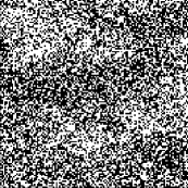
(b) Estimate obtained using the thresholding method; ${\varepsilon}_{N}=15.21$

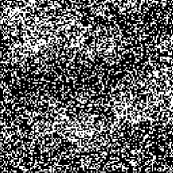
(c) Estimate obtained using the risk-optimal thresholding method; ${\varepsilon}_{N}=14.83$

(d) Estimate obtained using the wavelet-based method; ${\varepsilon}_{N}=4.824$

(e) Estimate obtained using the projective level set estimator; ${\varepsilon}_{N}=3.593$

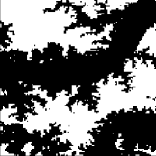
(f) Estimate obtained using the TV-based plug-in estimator; ${\varepsilon}_{N}=0.5596$

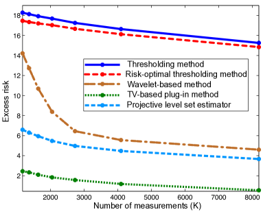
(g) Plot of excess risk as a function of $K<N=16384$ without performing the projected mean subtraction.

Figure 3: Snapshots of the simulation results obtained (without performing the projected mean subtraction) from observations of the form in (1).

Sparse support detection is the problem of detecting a set of locations $S^{*}_{N}={\left\{{i:f_{i}\neq 0}\right\}}$ corresponding to a discrete signal ${\bm{f}}\in{{\mathbb{R}}}^{N}$, given observations of the form in (1). This is a special case of level set estimation and the two are equivalent if ${\bm{f}}$ is nonnegative and $\gamma=0$. The idea of constructing proxy observations ${\bm{z}}$ to deduce certain properties of the underlying ${\bm{f}}$ has been successfully employed in recent compressed sensing and statistics literature to solve the problem of support detection of a discrete ${\bm{f}}$ having no more than $m$ non-zero entries; see, e.g., [bajwa:jc10, fletcher:tit09, wasserman, haupt2009compressive]. Specifically, it is established in [bajwa:jc10] that the support of an $m$-sparse ${\bm{f}}$ can be reliably and quickly detected from appropriately thresholded proxy observations with overwhelming probability as long as ${\bm{A}}$ satisfies a certain, easily verifiable coherence property. The success of this thresholding method stems primarily from the sparsity assumption on ${\bm{f}}$. However, when ${\bm{f}}$ is not sparse, as is the case in level set estimation, simply thresholding the proxy observations will result in numerous false positives and misses as discussed in detail in the numerical experiments in Sec. 7; see Figs. 2(a), 2(b), and Figs. 3(a) through 3(c). These results clearly suggest that we cannot simply use a support detection algorithm and an optimally chosen threshold to achieve an accurate level set estimation. In contrast, our methodology relies on a novel two-step approach that enables us to work with proxy observations without requiring ${\bm{f}}$ to be sparse.

3 Fast level set estimation from projection measurements

In order to extract the $\gamma$-level set of ${\bm{f}}$ from ${\bm{y}}$, we propose a novel two-step procedure. First, we construct a proxy of ${\bm{f}}$ according to (7), which allows us to arrive at the canonical signal plus noise observation model. Next, we perform level set estimation on the proxy observations ${\bm{z}}$, rather than on ${\bm{y}}$, using a method similar to the one derived in [willett:levelset]. We refer to the resulting estimator as the projective level set estimator. Note that for any unitary ${\bm{A}}$, ${\bm{z}}$ in (7) reduces to ${\bm{y}}={\bm{f}}+\tilde{{\bm{n}}}$ with $\tilde{{\bm{n}}}$ having independent, zero-mean entries. However, for non-unitary ${\bm{A}}$, the proxy defined in (7) creates a signal-dependent interference term $\left({\bm{A}}^{T}{\bm{A}}-{\bm{I}}\right){\bm{f}}$ and a zero-mean correlated noise term ${\bm{A}}^{T}{\bm{n}}$.

Intuitively, if we try to make a decision about each $z_{i}$ independently, then we would be vulnerable to noise (see, e.g., Figs. 3(b) and 3(c)). On the other hand, if we consider patches ${p_{j}}_{s}$ of $z_{i}$’s, defined as groups of $s$ proxy measurements ($z_{i}$’s) centered around $z_{j}$ for $s\in\{1,\ldots,N\}$, and force each patch to be wholly inside or outside the level set estimate, then we increase our robustness to noise but also increase our bias. Ideally, we want spatially adaptive patches that allow us to balance between an accurate approximation of the true level set boundary and estimator variance. It is in this vein that we theoretically analyze the impact of ${\bm{n}}^{\prime}$ on the level set estimation problem and use our analysis to develop a spatially-adaptive, dyadic, tree-based level set estimation approach that adapts to both the interference and the correlated noise term.

The algorithm we propose basically works by using ${\bm{z}}$ to find a partition of ${\bm{f}}$ into a collection of disjoint sets of “pixels.” For each set, we determine whether it is inside or outside the level set with a simple voting procedure—i.e., we determine whether the majority of the $z_{i}$’s in the set are greater than gamma. Thus searching for the optimal level set estimate amounts to searching for a good partition of ${\bm{f}}$ and then performing empirical risk minimization, defined in (9) in the sequel, on that partition. We restrict our attention to partitions defined using binary trees because they yield tractable algorithms and, in the case where ${\bm{A}}={\bm{I}}$, minimax optimality [willett:levelset].

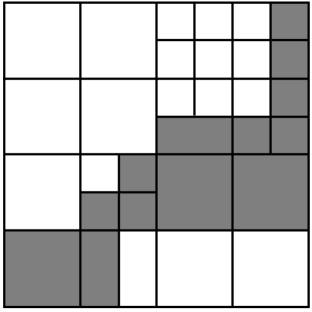
Figure 1: An example level set estimate ${S}\in\mathcal{S}_{M}$ where the domain of the underlying signal is $[0,1]^{2}$. Shaded regions are estimated to be outside the level set.

Specifically, let $\mathcal{S}_{M}$ be a collection of candidate level set estimates for a dyadic $M$ (i.e., $M=2^{q}$ for some positive integer $q$), where each ${S}\in\mathcal{S}_{M}$ is obtained by recursively partitioning the domain of ${\bm{f}}$ in dyadic intervals. The number of dyadic intervals along different coordinate directions is not required to be the same. In other words, each cell in the partition can potentially have different sidelengths and the sidelength of the smallest cell is $1/M$. An estimate ${S}\in\mathcal{S}_{M}$ is obtained by assigning each cell in the partition to be inside or outside of the level set. Fig. 1 shows one such estimate in two dimensions where the shaded regions are the partition cells that are estimated to be outside the level set. Though we do not specify $M$ in terms of $N$ here, we derive an upper bound on $M$ as a function of $N$ that achieves a certain expected excess risk in Theorem 2.

Given ${\bm{z}}$, our goal is to find a level set estimate

$$\widetilde{S}_{N}=\mathop{\rm arg\,min}_{{S}\in\mathcal{S}_{M}}R_{N}({S})-R_{N}(S^{*}_{N}){=\mathop{\rm arg\,min}_{{S}\in\mathcal{S}_{M}}R_{N}({S})}$$ (8)

where $R_{N}(\cdot)$ is defined in (4) and the second equality follows since $R_{N}(S^{*}_{N})$ is a constant. (Note that $\widetilde{S}_{N}=S^{*}_{N}$ if $S^{*}_{N}\in\mathcal{S}_{M}$.) Since ${\bm{f}}$ is unknown, $R_{N}({S})$ cannot be computed; instead, let us consider an empirical risk of the form

$$\widehat{R}_{N}({S})=\frac{1}{N}\sum_{i=1}^{N}\left(\gamma-z_{i}\right)\left[{{\mathbb{I}_{\left\{i\in{S}\right\}}}}-{{\mathbb{I}_{\left\{i\notin{S}\right\}}}}\right].$$ (9)

We show that finding an estimate that minimizes a penalized empirical risk results in an estimate that asymptotically approaches $\widetilde{S}_{N}$. Specifically, we find

$$\widehat{S}_{N}=\mathop{\rm arg\,min}_{{S}\in\mathcal{S}_{M}}\widehat{R}_{N}({S})+{{{\rm pen}}}_{N}({S}),$$ (10)

where ${{{\rm pen}}}_{N}({S})$ is an interference-dependent penalty term that yields ${\left|{R_{N}(\widehat{S}_{N})-R_{N}(\widetilde{S}_{N})}\right|}\stackrel{{\scriptstyle N\longrightarrow\infty}}{{\longrightarrow}}0$ subject to certain conditions on ${\bm{A}}$, which generally require $K\longrightarrow\infty$ as $N\longrightarrow\infty$. The penalty term plays a major role in our estimation strategy and is crucial in finding estimates that hone in on the boundary of the level set $S^{*}_{N}$. We thus focus on designing a spatially adaptive penalty ${{{\rm pen}}}_{N}({S})$ that promotes well-localized level sets with potentially non-smooth boundaries. Let $\pi({S})$ be the partition induced by an estimate ${S}\in\mathcal{S}_{M}$, i.e., $\pi({S})$ is the collection of all leaves in the estimate ${S}\in\mathcal{S}_{M}$. Fig. 1 shows a partition induced by one of the estimates ${S}\in\mathcal{S}_{M}$ where every white or gray shaded block is a leaf. We assign a label $\ell(L)$ to each leaf $L$ depending on whether $L$ is in the level set ($\ell(L)=1$) or otherwise ($\ell(L)=0$). Then the risk of ${S}$ in each of its leaf $L\in\pi({S})$ is given by

$$R_{N}(L)\stackrel{{\scriptstyle\scriptscriptstyle\triangle}}{{=}}\frac{1}{N}\sum_{i=1}^{N}\left(\gamma-f_{i}\right)\left[{{\mathbb{I}_{\left\{\ell(L)=1\right\}}}}-{{\mathbb{I}_{\left\{\ell(L)=0\right\}}}}\right]{{\mathbb{I}_{\left\{i\in L\right\}}}}.$$

Note that $R_{N}({S})=\sum_{L\in\pi({S})}R_{N}(L)$. We design a spatially adaptive penalty term by analyzing $R_{N}(L)-\widehat{R}_{N}(L)$ within each leaf separately. To facilitate our analysis, let us define

$$\widetilde{R}_{N}(L)\stackrel{{\scriptstyle\scriptscriptstyle\triangle}}{{=}}\frac{1}{N}\sum_{i=1}^{N}\left(\gamma-{{\mathbb{E}}}\left[{z_{i}}\right]\right)\left[{{\mathbb{I}_{\left\{\ell(L)=1\right\}}}}-{{\mathbb{I}_{\left\{\ell(L)=0\right\}}}}\right]{{\mathbb{I}_{\left\{i\in L\right\}}}}.$$

Then

$${\left|{R_{N}(L)-\widehat{R}_{N}(L)}\right|} ={\left|{R_{N}(L)-\widetilde{R}_{N}(L)+\widetilde{R}_{N}(L)-\widehat{R}_{N}(L)}\right|}$$

$$= {\left|{\frac{1}{N}\sum_{i=1}^{N}{\left[{\left({{\mathbb{E}}}\left[{z_{i}}\right]-f_{i}\right)+\left(z_{i}-{{\mathbb{E}}}\left[{z_{i}}\right]\right)}\right]}\left[{{\mathbb{I}_{\left\{\ell(L)=1\right\}}}}-{{\mathbb{I}_{\left\{\ell(L)=0\right\}}}}\right]{{\mathbb{I}_{\left\{i\in L\right\}}}}}\right|}$$

$$\leq \underbrace{{\left|{\frac{1}{N}\sum_{i=1}^{N}\left({{\mathbb{E}}}\left[{z_{i}}\right]-f_{i}\right)\left[{{\mathbb{I}_{\left\{\ell(L)=1\right\}}}}-{{\mathbb{I}_{\left\{\ell(L)=0\right\}}}}\right]{{\mathbb{I}_{\left\{i\in L\right\}}}}}\right|}}_{T_{1}}$$ (11)

$$+\underbrace{{\left|{\frac{1}{N}\sum_{i=1}^{N}\left(z_{i}-{{\mathbb{E}}}\left[{z_{i}}\right]\right)\left[{{\mathbb{I}_{\left\{\ell(L)=1\right\}}}}-{{\mathbb{I}_{\left\{\ell(L)=0\right\}}}}\right]{{\mathbb{I}_{\left\{i\in L\right\}}}}}\right|}}_{T_{2}}.$$

Note that while $T_{1}$ is a measure of the bias in ${\bm{z}}$, $T_{2}$ is a measure of the concentration of ${\bm{z}}$ about its mean. Since the columns of ${\bm{A}}$ are assumed to have unit $\ell_{2}$ norms, one can easily see from (7) that

$$z_{i}=f_{i}+\sum_{j=1,j\neq i}^{N}f_{j}{\left\langle{{\bm{A}}^{(i)},{\bm{A}}^{(j)}}\right\rangle}+{\left\langle{{\bm{A}}^{(i)},{\bm{n}}}\right\rangle}$$ (12)

where ${\bm{A}}^{(i)}$ denotes the ${{i^{{\rm th}}}}$ column of ${\bm{A}}$ and ${\left\langle{\cdot,\cdot}\right\rangle}$ denotes the usual innerproduct. Since ${\bm{A}}$ is given, and ${\bm{n}}$ is zero mean, the term

$${{\mathbb{E}}}\left[{z_{i}}\right]-f_{i}=\sum_{j=1,j\neq i}^{N}f_{j}{\left\langle{{\bm{A}}^{(i)},{\bm{A}}^{(j)}}\right\rangle}$$ (13)

in $T_{1}$ is the signal-dependent interference term at the ${{i^{{\rm th}}}}$ location due to the signal energies at other locations. We upper bound $T_{1}$ by the $\ell_{1}$ norm of ${\bm{f}}$ and the worst-case coherence of ${\bm{A}}$ (defined in the statement of Theorem 1), bound $T_{2}$ using a Hoeffding-like inequality for a weighted sum of independent subGaussian random variables [rudelson2013lecture], and sum the risk in each leaf of the estimate ${S}$ to arrive at the following result.

Theorem 1 (Concentration of risk around the empirical risk)

Suppose that the entries of noise ${\bm{n}}$ are subGaussian distributed with parameter $c_{s}$. Then, for $\delta\in[0,1/2]$ and $c>0$, with probability at least $1-2\delta$, the following holds for all ${S}\in\mathcal{S}_{M}$:

$${\left|{R_{N}({S})-\widehat{R}_{N}({S})}\right|}\leq \left(\frac{N-1}{N}\right)\mu({\bm{A}})\|{\bm{f}}\|_{1}+{{{\rm pen}}}_{N}({S})$$ (14)

where ${\left\|{{\bm{f}}}\right\|}_{1}=\sum_{i}{\left|{f_{i}}\right|}$ is the $\ell_{1}$ norm of ${\bm{f}}$,

$${{{\rm pen}}}_{N}({S})\stackrel{{\scriptstyle\scriptscriptstyle\triangle}}{{=}}\sum_{L\in\pi({S})}\frac{1}{N}\sqrt{\frac{\left[\log(2/\delta)+\llbracket L\rrbracket\log 2\right]{{\color[rgb]{0,0,0}c_{s}^{2}}}\sum_{i,j\in L}{\left\langle{{\bm{A}}^{(i)},{\bm{A}}^{(j)}}\right\rangle}}{2c}}$$ (15)

is the penalty term,

$$\mu({\bm{A}})\stackrel{{\scriptstyle\scriptscriptstyle\triangle}}{{=}}\max_{i,j\in\{1,\ldots,N\},i\neq j}{\left|{{\left\langle{{\bm{A}}^{(i)},{\bm{A}}^{(j)}}\right\rangle}}\right|}$$

is the worst-case coherence of ${\bm{A}}$ and $\llbracket L\rrbracket$ is the number of bits in a prefix code used to uniquely encode the position of a leaf $L$ in the tree.

The proof of this theorem is provided in Section 5.1. The above bound holds for any prefix code $\llbracket L\rrbracket$. In order to achieve the error rates in Theorem 2, we use a certain prefix code, which is discussed before the statement of Theorem 2. Note that the bounds in (14) and (15) depend on (a) the signal-dependent interference term in (7) through ${\left\|{{\bm{f}}}\right\|}_{1}$, (b) the noise statistics through $c_{s}$, (c) the choice of ${\bm{A}}$ through $\mu({\bm{A}})$, (d) the depth of each leaf through $\llbracket L\rrbracket$, (e) the size of each leaf through $\sum_{i,j\in L}{\left\langle{{\bm{A}}^{(i)},{\bm{A}}^{(j)}}\right\rangle}$ and (f) the parameter $\delta$. Ideally we would like to minimize $R_{N}({S})$ to obtain $\widetilde{S}_{N}$ in (8). Since $R_{N}({S})$ is bounded by $\widehat{R}_{N}({S})+{{{\rm pen}}}_{N}({S})$, minimizing the bound (14) will ensure that our estimate $\widehat{S}_{N}$ in (10) is as close to $\widetilde{S}_{N}$ in (8) as possible. In order to minimize the risk difference in (14), one needs to choose an estimate ${S}\in\mathcal{S}_{M}$ that has the least ${{{\rm pen}}}_{N}({S})$ in (15). The penalty term in (15) is directly proportional to the number of leaves in the partition $\pi({S})$ and the size of each leaf through the term $\sum_{i,j\in L}{\left\langle{{\bm{A}}^{(i)},{\bm{A}}^{(j)}}\right\rangle}$. As a result, searching for an estimate ${S}\in\mathcal{S}_{M}$ that minimizes (10) will favor estimates with few, deep leaves that hone in on the boundary of the level set.

The theoretical analysis of our method is significantly different from the analysis in [willett:levelset] because of the statistics of the noise term ${\bm{n}}^{\prime}$ in our problem. However, this only changes the way the penalty is defined in our setup. As a result, we can adapt the computational techniques discussed in [willett:levelset] to compute our estimator in an efficient way. Our method is computationally efficient since the proxy computation needs at most $O(KN)$ operations (fewer if ${\bm{A}}$ is structured; e.g., ${\bm{A}}$ is a Toeplitz matrix) and the level set estimation method needs $O(N\log N)$ operations, as noted in [willett:levelset].

3.1 Performance analysis

As discussed earlier in Sec. 1.1, our eventual goal is to estimate the continuous-domain level set $S^{*}$ from discrete measurements ${\bm{y}}$. In this section, we show that estimating the discrete-domain level set $S^{*}_{N}$ helps us achieve this goal by establishing that ($i$) $S^{*}_{N}\longrightarrow S^{*}$ as $N\longrightarrow\infty$ and ($ii$) providing conditions, as a function of problem parameters, under which the discrete-domain level set estimate obtained according to (10) approaches $S^{*}$. To this end, we can utilize the results of Theorem 1 to upper bound the expected excess risk ${{\mathbb{E}}}\left[{R(\widehat{S}_{N})-R(S^{*})}\right]$, taken with respect to the noise distribution, in terms of the problem parameters, where

$$R(S)=\int_{{\left[{0,1}\right]}^{d}}{\left({\gamma-f(x)}\right)}{\left[{{{\mathbb{I}_{\left\{x\in S\right\}}}}-{{\mathbb{I}_{\left\{x\notin S\right\}}}}}\right]}dx$$

is the definition of risk in continuous-domain. The expected excess risk is a measure of the effectiveness of our level set estimator. Before studying it, we make certain assumptions about the smoothness of $f$ in the vicinity of the level set boundary. Let $\partial S^{*}$ represent the level set boundary corresponding to $S^{*}={\left\{{x:f(x)>\gamma}\right\}}$. We assume that $f$ is in a box-counting function class ${\mathcal{D}}_{{{\rm BOX}}}(\kappa,\gamma,c_{1},c_{2})$ for $c_{1},c_{2}>0$ and $1\leq\kappa\leq\infty$ [willett:levelset] such that the following hold:

1. If we partition $[0,1]^{d}$ to $m^{d}$ equisized cells for $m\leq M$, with each of them having a sidelength of $1/m$ and volume $m^{-d}$, then the number of such cells intersected by the level set boundary $N_{S^{*}}(m)\leq c_{1}m^{d-1}$. This ensures that $\partial S^{*}$ varies smoothly and is not an irregular, space-filling curve.

2. For all dyadic $m$, let

   $$S_{m}^{*}=\mathop{\rm arg\,min}_{{S}\in\mathcal{S}_{m}}\lambda{\left({\Delta{\left({{S},S^{*}}\right)}}\right)}$$ (16)

   be a candidate in $\mathcal{S}_{m}$ that minimizes the symmetric difference between any $S\in\mathcal{S}_{m}$ and the true level set $S^{*}$ in terms of the Lebesgue measure $\lambda$. For this $S_{m}^{*}$, the excess risk in the continuous domain follows

   $${\varepsilon}{\left({{S_{m}^{*}},S^{*}}\right)}=R(S_{m}^{*})-R(S^{*})\stackrel{{\scriptstyle\scriptscriptstyle\triangle}}{{=}}\int_{\Delta(S^{*}\!,S_{m}^{*})}{\left|{\gamma-f(x)}\right|}dx\leq c_{2}m^{-\kappa}.$$ (17)

Parameter $\kappa$ and the assumption on the excess risk in (17) allow us to study the fluctuations of $f$ around $\partial S^{*}$ and thus examine the behavior of ${\varepsilon}{\left({{S_{m}^{*}},{S^{*}}}\right)}$ in the vicinity of the level set boundary. If $f$ exhibits a very small fluctuation around $\partial S^{*}$, then ${\varepsilon}{\left({{S_{m}^{*}},{S^{*}}}\right)}$ is small even if the symmetric difference $\Delta({S^{*}\!},S_{m}^{*})$ is very large, since the excess risk is weighted by how close is $f$ to $\gamma$. In other words, a high value of $\kappa$ indicates that $f$ varies very smoothly around the level set boundary and a low value of $\kappa$ means that there is a jump in $f$ around $\partial S^{*}$.

Recall that $S^{*}_{N}$ is obtained by partitioning the space $[0,1]^{d}$ to $N$ equisized cells of sidelengths $N^{-d}$ and assigning each cell to be inside or outside of the level set. From (17), for $m=N^{1/d}$,

$$R(S^{*}_{N})-R(S^{*})\leq c_{2}N^{-\kappa/d}.$$

Thus $S^{*}_{N}\longrightarrow S^{*}$ as $N\longrightarrow\infty$ and estimation of $S^{*}$ via $S^{*}_{N}$ is reasonable.

To achieve the results of Theorem 2 stated below, we adapt the prefix code proposed in [willett:levelset, scott2006minimax]. According to [willett:levelset, scott2006minimax], a leaf $L$ of a level set at depth $j$ of the tree can be uniquely encoded using a total of $j(\log_{2}d+2)+1$ bits. Specifically, one needs $j+1$ bits to encode the depth of the leaf, $j$ bits to encode whether each of its ancestors corresponded to a left or a right branch of the tree, and $j\log_{2}d$ bits to encode the orientation of each of the $j$ branches.

Before we state our main theorem, let us clarify the notation used in the following. For a given set of sequences $a_{n}$ and $b_{n}$, $a_{n}\preccurlyeq b_{n}$ implies that there exists a constant $C>0$ such that $a_{n}\leq Cb_{n}$ for all $n$ and $a_{n}\asymp b_{n}$ implies that there exists constants $C_{1}$ and $C_{2}$ such that $C_{1}a_{n}\leq b_{n}\leq C_{2}a_{n}$ for all $n$.

Theorem 2 (Upper bound on the expected excess risk)

If $f\in{\mathcal{D}}_{{{\rm BOX}}}(\kappa,\gamma,c_{1},c_{2})$ is discretized according to (2), $-B\leq f(x)\leq B$ for $x\in[0,1]^{d}$, $-B\leq\gamma\leq B$, and the estimate $\widehat{S}_{N}$ is chosen according to (10) with ${{{\rm pen}}}_{N}(\widehat{S}_{N})$ defined according to Theorem. 1, then, for a given ${\bm{A}}$, $d\geq 2$, and for $M\succcurlyeq{\left({\frac{N}{{\left\|{{\bm{A}}}\right\|}_{2}^{2}\log N}}\right)}^{1/d}$,

$${{\mathbb{E}}}{\left[{R(\widehat{S}_{N})-R(S^{*})}\right]} \preccurlyeq{\left({\frac{{\left\|{{\bm{A}}}\right\|}_{2}^{2}\log N}{N}}\right)}^{\frac{\kappa}{2\kappa+d-2}}+\mu({\bm{A}}){\left\|{{\bm{f}}}\right\|}_{1}$$ (18)

where the expectation is with respect to the noise distribution, ${\left\|{{\bm{A}}}\right\|}_{2}$ is the spectral norm of ${\bm{A}}$, $\|{\bm{A}}\|_{2}\stackrel{{\scriptstyle\scriptscriptstyle\triangle}}{{=}}\sqrt{\lambda_{\max}\left({\bm{A}}^{T}{\bm{A}}\right)}$, and $\mu({\bm{A}})$ is the worst-case coherence of ${\bm{A}}$.

The proof of this theorem is given in Section 5.2. This theorem tells us how the expected excess risk scales with the dimensionality $N$ of the underlying signal ${\bm{f}}$, the $\ell_{1}$ norm of ${\bm{f}}$, the choice of ${\bm{A}}$ and the smoothness of the underlying function around the level set boundary through the parameter $\kappa$. For a unitary matrix ${\bm{A}}$, ${\left\|{{\bm{A}}}\right\|}_{2}=1$ since its singular values are all equal to $1$, $\mu({\bm{A}})=0$ and ${{\mathbb{E}}}{\left[{R(\widehat{S}_{N})-R(S^{*})}\right]}\preccurlyeq{\left({\frac{\log N}{N}}\right)}^{\frac{\kappa}{2\kappa+d-2}}$, which is the minimax optimal rate derived in [willett:levelset] without the projection matrix ${\bm{A}}$. Since in practice ${\bm{A}}$ is dictated by the physics of the measurement system, it is not always unitary. In such cases, the above theorem tells us how any given ${\bm{A}}$ increases this bound. For some ${\bm{A}}$, such as the one discussed in the following section, $\mu({\bm{A}})\longrightarrow 0$ as $N$ and $K$ go to $\infty$ since ${\bm{A}}^{T}{\bm{A}}\stackrel{{\scriptstyle N,K\longrightarrow\infty}}{{\longrightarrow}}{\bm{I}}$. Note that (18) can be specified in terms of the continuous-domain function $f$ by noting that ${\left\|{{\bm{f}}}\right\|}_{1}\leq N{\left\|{f}\right\|}_{L_{1}}$, although it is a loose bound when the function $f$ is not completely positive (or negative).

Corollary 1 (Performance with random projections)

If the entries of ${\bm{A}}\in{{\mathbb{R}}}^{K\times N}$ are drawn from ${{\mathcal{N}}\left({0,1/K}\right)}$, and the columns of ${\bm{A}}$ are normalized to have unit $\ell_{2}$ norm, then

$${{\mathbb{E}}}{\left[{R(\widehat{S}_{N})-R(S^{*})}\right]}\preccurlyeq{\left({\frac{\log N}{N}}\right)}^{\frac{\kappa}{2\kappa+d-2}} {\left[{\frac{\sqrt{K}+\sqrt{N}}{\sqrt{K-\sqrt{12K\log N}}}}\right]}^{\frac{2\kappa}{2\kappa+d-2}}+$$

$$\qquad\frac{\sqrt{15\log N}}{\sqrt{K}-\sqrt{12\log N}}{\left\|{{\bm{f}}}\right\|}_{1}$$ (19)

holds with probability at least $1-{\left[{e^{-c{\left({K+N}\right)}}+N^{-2}+11N^{-1}}\right]}$ as long as $60\log N\leq K\leq\frac{N-1}{4\log N}$.

The proof of this corollary is provided in Sec. 5.3. The result above yields an upper bound on the expected excess risk as a function of the dimensions of the projection operator ${\bm{A}}$ and ${\left\|{{\bm{f}}}\right\|}_{1}$. In words, this corollary states that the expected excess risk in the case of random Gaussian projections is minimized if the number of measurements $K$ scales linearly with $N$ and increases if $K$ scales sublinearly with $N$. Dependence of the estimator’s performance on the $\ell_{1}$ norm of ${\bm{f}}$ is due to the interference term $\left({\bm{A}}^{T}{\bm{A}}-{\bm{I}}\right){\bm{f}}$ that arises during the proxy construction. The foregoing results provide key insights into ways by which we can minimize the expected excess risk and improve performance, as discussed in detail in the following section.

We conclude our discussion of Theorem 2 by pointing out that practically meaningful lower bounds for this problem are unknown at this time, but would be the subject of a future investigation. In addition, note that our focus in here has been on very fast, easily implementable methods for real-time estimation of level sets. While significantly slower methods could conceivably be developed to potentially provide lower errors, such methods would not be able to compete with our proposed approach in terms of the computational costs (see, e.g., Sec. 7).

4 Performance improvement via projected median subtraction

So far we have shown that the signal-dependent interference term in (7) leads to a penalty term proportional to ${\left\|{{\bm{f}}}\right\|}_{1}$ in (14). This implies that the interference in ${\bm{z}}$ and thus the performance of our method may worsen with the increase in ${\left\|{{\bm{f}}}\right\|}_{1}$, which is indeed confirmed by the experimental results in Sec. 7. To find a way to minimize the signal-dependent interference, let us write ${\bm{f}}={\bm{\widetilde{f}}}+\lambda\mathbbm{1}$, where $\lambda$ is a constant DC offset such that

$${\left\|{{\bm{\widetilde{f}}}}\right\|}_{1}\leq{\left\|{{\bm{f}}}\right\|}_{1}.$$ (20)

If we have access to an estimate $\widehat{\lambda}$ of $\lambda$, then we can minimize the signal-dependent interference by subtracting a projection of this constant offset to obtain

$${\bm{\widetilde{y}}} ={\bm{y}}-{\bm{A}}{\widehat{\lambda}\mathbbm{1}}={\bm{A}}{\left({{\bm{\widetilde{f}}}+\lambda\mathbbm{1}}\right)}+{\bm{n}}-{\bm{A}}\widehat{\lambda}\mathbbm{1}$$

$$={\bm{A}}{\left({{\bm{\widetilde{f}}}+{\left({\lambda-\widehat{\lambda}}\right)}\mathbbm{1}}\right)}+{\bm{n}}\approx{\bm{A}}{\bm{\widetilde{f}}}+{\bm{n}},$$

assuming that $\widehat{\lambda}\approx\lambda$. The proxy observations in this case reduce to

$$\widetilde{{\bm{z}}} ={\bm{A}}^{T}{\bm{\widetilde{y}}}\approx{\bm{A}}^{T}{\bm{A}}{\bm{\widetilde{f}}}+{\bm{A}}^{T}{\bm{A}}{\bm{n}}={\bm{\widetilde{f}}}+{\left({{\bm{A}}^{T}{\bm{A}}-{\bm{I}}}\right)}{\bm{\widetilde{f}}}+{\bm{A}}^{T}{\bm{A}}{\bm{n}}.$$

Since $S^{*}_{N}=\{i:f_{i}>\gamma\}\stackrel{{\scriptstyle\scriptscriptstyle\triangle}}{{=}}\{i:{\widetilde{f}}_{i}>\widetilde{\gamma}\}$, where $\widetilde{\gamma}=\gamma-\lambda$, we can estimate $S^{*}_{N}$ from $\widetilde{{\bm{z}}}$ using our level set estimation method discussed in the previous section.

If we let $\lambda$ to be the median of ${\bm{f}}$, then we can easily show that (20) holds for this particular choice of $\lambda$. Note that if $\lambda$ is the median of ${\bm{f}}$, then half the pixel values of ${\bm{f}}$ are below the median and half of the pixel values are above the median. Let ${\mathcal{G}}={\left\{{i:f_{i}>\lambda}\right\}}$ and ${\mathcal{G}}^{c}={\left\{{i:f_{i}<\lambda}\right\}}$. The cardinality of ${\mathcal{G}}$ is ${\left|{{\mathcal{G}}}\right|}=N/2$ for $N$ even. By the definition of median, ${\left|{{\mathcal{G}}}\right|}={\left|{{\mathcal{G}}^{c}}\right|}$. Then

$${\left\|{{\bm{\widetilde{f}}}}\right\|}_{1} ={\left\|{{\bm{f}}-\lambda\mathbbm{1}}\right\|}_{1}=\sum_{i\in{\mathcal{G}}}{\left|{f_{i}-\lambda}\right|}+\sum_{i\in{\mathcal{G}}^{c}}{\left|{f_{i}-\lambda}\right|}$$

$$=\sum_{i\in{\mathcal{G}}}{\left({f_{i}-\lambda}\right)}+\sum_{i\in{\mathcal{G}}^{c}}{\left({\lambda-f_{i}}\right)}=\sum_{i\in{\mathcal{G}}}f_{i}+\sum_{i\in{\mathcal{G}}^{c}}-f_{i}-{\left|{{\mathcal{G}}}\right|}\lambda+{\left|{{\mathcal{G}}^{c}}\right|}\lambda$$

$$=\sum_{i\in{\mathcal{G}}}f_{i}+\sum_{i\in{\mathcal{G}}^{c}}-f_{i}$$

$$\leq\sum_{i\in{\mathcal{G}}}{\left|{f_{i}}\right|}+\sum_{i\in{\mathcal{G}}^{c}}{\left|{f_{i}}\right|}={\left\|{{\bm{f}}}\right\|}_{1}.$$

In practice, however, estimation of the median of ${\bm{f}}$ from ${\bm{y}}$ might be hard, though the estimation of the mean of ${\bm{f}}$ might be tractable. For instance, if we construct ${\bm{A}}^{\prime}=\left[\begin{smallmatrix}\mathbbm{1}^{T}\\ {\bm{A}}\end{smallmatrix}\right]$ (i.e., the first row of ${\bm{A}}^{\prime}$ is $\mathbbm{1}^{T}$), then ${\bm{y}}^{\prime}={\bm{A}}^{\prime}{\bm{f}}+{\bm{n}}=\left[\begin{smallmatrix}y^{\prime}_{1}\\ {\bm{y}}\end{smallmatrix}\right]$, and $\widehat{\lambda}=y^{\prime}_{1}/N={\left({\sum_{i}f_{i}+n_{1}}\right)}/N=\lambda+n_{1}/N$. If the observation noise is negligible, or if $N$ is large, then $\widehat{\lambda}\approx\lambda$ and we can perform projected mean subtraction, instead of a projected median subtraction, to reduce the signal-dependent interference. While (20) does not always hold if $\lambda$ is the mean of ${\bm{f}}$, simulation results in Sec. 7 suggest that projected mean subtraction can result in significant improvement in performance.

5 Proofs of theorems and corollaries

This section presents the proofs of all the theorems and corollaries stated before.

5.1 Proof of Theorem 1 (Concentration of risk )

Let us begin by bounding $T_{1}$ and $T_{2}$ in (11) separately. Let $\widehat{p}_{L}=\sum_{i\in L}\frac{1}{N}$ be the ratio of the number of observations in leaf $L$ to the total number of observations $N$. From the statistics of $z$, we can bound $T_{1}$ as follows:

$$T_{1}\leq\frac{1}{N}\sum_{i,j:j\neq i}{\left|{f_{j}}\right|}{\left|{{\left\langle{{\bm{A}}^{(i)},{\bm{A}}^{(j)}}\right\rangle}}\right|}{\left|{\left[{{\mathbb{I}_{\left\{\ell(L)=1\right\}}}}-{{\mathbb{I}_{\left\{\ell(L)=0\right\}}}}\right]}\right|}{{\mathbb{I}_{\left\{i\in L\right\}}}}$$

$$\leq\frac{\mu({\bm{A}})}{N}\sum_{i\in L}\sum_{j=1:j\neq i}^{N}|f_{j}|=\frac{\mu({\bm{A}})}{N}\sum_{i\in L}\left(\sum_{j=1}^{N}{\left|{f_{j}}\right|}-{\left|{f_{i}}\right|}\right)$$

$$\leq\mu({\bm{A}})\widehat{p}_{L}\|{\bm{f}}\|_{1}-\frac{\mu({\bm{A}})}{N}\sum_{i\in L}{\left|{f_{i}}\right|},$$ (21)

where the second inequality is due to the fact that ${\left|{\left[{{\mathbb{I}_{\left\{\ell(L)=1\right\}}}}-{{\mathbb{I}_{\left\{\ell(L)=0\right\}}}}\right]}\right|}=1$ and ${\left|{{\left\langle{{\bm{A}}^{(i)},{\bm{A}}^{(j)}}\right\rangle}}\right|}\leq\mu({\bm{A}})$ for all $j\neq i$.

Rewriting $T_{2}$ in terms of (12) and (13) we have

$$T_{2} =\frac{1}{N}\sum_{i\in L}\left(\sum_{k=1}^{K}a_{k,i}n_{k}\right)\left[{{\mathbb{I}_{\left\{\ell(L)=1\right\}}}}-{{\mathbb{I}_{\left\{\ell(L)=0\right\}}}}\right]=\sum_{k=1}^{K}b_{k}n_{k}$$

where $b_{k}=\frac{1}{N}\sum_{i\in L}a_{k,i}\left[{{\mathbb{I}_{\left\{\ell(L)=1\right\}}}}-{{\mathbb{I}_{\left\{\ell(L)=0\right\}}}}\right]$. Observe that $T_{2}$ is a weighted sum of $K$ independent, zero-mean, subGaussian random variables. It then follows from a Hoeffding-like inequality for a weighted sum of independent, zero-mean subGaussian random variables [rudelson2013lecture, Theorem 3.3] that

$${{\mathbb{P}}}{\left({{\left|{\sum_{k=1}^{K}b_{k}n_{k}}\right|}\geq\epsilon}\right)}\leq 2\exp{\left({\frac{-c\epsilon^{2}}{c_{s}^{2}\sum_{k=1}^{K}b_{k}^{2}}}\right)}$$ (22)

for $\epsilon>0$, where $c>0$ is an absolute numerical constant. Let us now evaluate the term $\sum_{k=1}^{K}b_{k}^{2}$ in the above expression as follows:

$$\sum_{k=1}^{K}b_{k}^{2} =\sum_{k=1}^{K}{\left({\frac{1}{N}\sum_{i\in L}a_{k,i}\left[{{\mathbb{I}_{\left\{\ell(L)=1\right\}}}}-{{\mathbb{I}_{\left\{\ell(L)=0\right\}}}}\right]}\right)}^{2}$$

$$=\frac{1}{N^{2}}\sum_{k=1}^{K}\sum_{i\in L}a_{k,i}\left[{{\mathbb{I}_{\left\{\ell(L)=1\right\}}}}-{{\mathbb{I}_{\left\{\ell(L)=0\right\}}}}\right]\sum_{j\in L}a_{k,j}\left[{{\mathbb{I}_{\left\{\ell(L)=1\right\}}}}-{{\mathbb{I}_{\left\{\ell(L)=0\right\}}}}\right]$$

$$=\frac{1}{N^{2}}\sum_{k=1}^{K}\sum_{i\in L}\sum_{j\in L}a_{k,i}a_{k,j}=\frac{1}{N^{2}}\sum_{i\in L}\sum_{j\in L}{\left\langle{{\bm{A}}^{(i)},{\bm{A}}^{(j)}}\right\rangle}$$ (23)

where the above equation is due to the fact that $\left[{{\mathbb{I}_{\left\{\ell(L)=1\right\}}}}-{{\mathbb{I}_{\left\{\ell(L)=0\right\}}}}\right]^{2}=1$. By substituting (23) in (22) and by equating the right hand side of (22) to $\delta_{L}\in(0,1/2)$ and solving for $\epsilon$, we can show that, with probability at least $1-2\delta_{L}$,

$$T_{2}\leq\sqrt{\frac{\log(1/\delta_{L})c_{s}^{2}\sum_{i,j\in L}{\left\langle{{\bm{A}}^{(i)}{,\,}{\bm{A}}^{(j)}}\right\rangle}}{2cN^{2}}}.$$ (24)

Applying the bounds in (21) and (24) to (11) we can see that with probability at least $1-2\delta_{L}$, the following holds:

$${\left|{R_{N}(L)-\widehat{R}_{N}(L)}\right|}\leq \left(\mu({\bm{A}})\widehat{p}_{L}\|{\bm{f}}\|_{1}-\frac{\mu({\bm{A}})}{N}\sum_{i\in L}{\left|{f_{i}}\right|}\right)$$

$$+\sqrt{\frac{\log(1/\delta_{L})c_{s}^{2}\sum_{i,j\in L}{\left\langle{{\bm{A}}^{(i)}{,\,}{\bm{A}}^{(j)}}\right\rangle}}{2N^{2}}}.$$

Thus for a given ${S}\in\mathcal{S}_{M}$, the risk difference ${\left|{R_{N}({S})-\widehat{R}_{N}({S})}\right|}$ is upper bounded by summing the bound corresponding to each leaf separately. Since $\sum_{L\in\pi({S})}\widehat{p}_{L}=1$ and $\sum_{L\in\pi({S})}\sum_{i\in L}{\left|{f_{i}}\right|}={\left\|{{\bm{f}}}\right\|}_{1}$ we have

$${\left|{R_{N}({S})-\widehat{R}_{N}({S})}\right|}\leq \mu({\bm{A}})\left(\frac{N-1}{N}\right){\left\|{{\bm{f}}}\right\|}_{1}+\sum_{L\in\pi({S})}\sqrt{\frac{\log(1/\delta_{L})c_{s}^{2}\sum_{i,j\in L}{\left\langle{{\bm{A}}^{(i)}{,\,}{\bm{A}}^{(j)}}\right\rangle}}{2N^{2}}}$$

with high probability. If we let $\delta_{L}=\delta 2^{-(\llbracket L\rrbracket+1)}$ where $\llbracket L\rrbracket$ is the number of bits required to uniquely encode the position of leaf $L$, then it is straightforward to follow the proof of Lemma 2 in [willett:levelset] to show that the bound above holds for every ${S}\in\mathcal{S}_{M}$, which leads to the result of Theorem 1.

5.2 Proof of Theorem 2 (Performance analysis)

In order to analyze the performance of our estimator, we will draw upon the proof techniques and the associated performance analyses in previous works on classification and level set estimation [scott2006minimax, willett:levelset]. Note that some of the steps in our analysis that are adapted from [scott2006minimax, willett:levelset] are repeated here for readability.

The proof of this theorem follows by relating the continuous-domain risk of a level set ${S}\in\mathcal{S}_{M}$ to its discrete counterpart and exploiting the results from Theorem 1. By expanding $R(S)$ for any $S\in\mathcal{S}_{M}$ in terms of the discretization of $f$ in (2), we have,

$$R(S) =\int_{x}(\gamma-f(x)){\left[{{{\mathbb{I}_{\left\{x\in S\right\}}}}-{{\mathbb{I}_{\left\{x\notin S\right\}}}}}\right]}dx$$

$$=\sum_{i=1}^{N}\int_{C_{i}}(\gamma-f(x)){\left[{{{\mathbb{I}_{\left\{C_{i}\in S\right\}}}}-{{\mathbb{I}_{\left\{C_{i}\notin S\right\}}}}}\right]}dx$$

$$=\sum_{i=1}^{N}{\left({\gamma\textrm{vol}\left(C_{i}\right)-\textrm{vol}\left(C_{i}\right)f_{i}}\right)}{\left[{{{\mathbb{I}_{\left\{C_{i}\in S\right\}}}}-{{\mathbb{I}_{\left\{C_{i}\notin S\right\}}}}}\right]}$$

$$=\sum_{i=1}^{N}{\left({\frac{\gamma}{N}-\frac{f_{i}}{N}}\right)}{\left[{{{\mathbb{I}_{\left\{i\in S\right\}}}}-{{\mathbb{I}_{\left\{i\notin S\right\}}}}}\right]}\equiv R_{N}(S)$$

where the second equality holds since $C_{i}$ is contained either in $S$ or in the complement of $S$. Since $\widehat{S}_{N}\in\mathcal{S}_{M}$, $R(\widehat{S}_{N})=R_{N}(\widehat{S}_{N})$. Let us consider some $S_{N}^{\prime}\in\mathcal{S}_{M}$ that minimizes the penalized excess risk between any $S\in\mathcal{S}_{M}$ and the true level set $S^{*}$, i.e.,

$$S_{N}^{\prime}=\min_{S\in\mathcal{S}_{M}}{\left[{R(S)-R(S^{*})+2{{{\rm pen}}}_{N}(S)}\right]}.$$

From the definitions of $\widehat{S}_{N}$ in (10) and $S_{N}^{\prime}$, and the results of Theorem 1, the following holds with probability at least $1-2\delta$ for $\delta\in[0,1/2]$:

$$R(\widehat{S}_{N})-R(S^{*}) =R_{N}(\widehat{S}_{N})-R(S^{*})\leq\min_{S\in\mathcal{S}_{M}}{\left[{R(S)-R(S^{*})+2{{{\rm pen}}}_{N}(S)}\right]}.$$ (25)

Let $\Omega$ denote the event that (14) from Theorem 1 holds for all proxy observations ${\bm{z}}$. Since $-B\leq f(x)\leq B$ for all $x\in[0,1]^{d}$ and $-B\leq\gamma\leq B$, for $\delta=1/N$

$${{\mathbb{E}}} {\left[{R(\widehat{S}_{N})-R(S^{*})}\right]}={{\mathbb{E}}}{\left[{R_{N}(\widehat{S}_{N})-R(S^{*})}\right]}$$

$$={{\mathbb{E}}}{\left[{R_{N}(\widehat{S}_{N})-R(S^{*})|\Omega}\right]}{{\mathbb{P}}}(\Omega)+{{\mathbb{E}}}{\left[{R_{N}(\widehat{S}_{N})-R(S^{*})|\Omega^{c}}\right]}{{\mathbb{P}}}(\Omega^{c})$$

$$\leq{{\mathbb{E}}}{\left[{R_{N}(\widehat{S}_{N})-R(S^{*})|\Omega}\right]}+{{\mathbb{E}}}{\left[{R_{N}(\widehat{S}_{N})-R(S^{*})|\Omega^{c}}\right]}\frac{2}{N}$$

$$\leq\min_{S\in\mathcal{S}_{M}}\left[R(S)-R(S^{*})+2{{{\rm pen}}}_{N}(S)\right]+4B\times\frac{2}{N}$$ (26)

where the first term in (26) is due to (25) and the second term is due to the boundedness assumption on $f(x)$ and $\gamma$. Specifically,

$$R_{N}(\widehat{S}_{N})-R(S^{*}) \equiv R(\widehat{S}_{N})-R(S^{*})$$

$$=\int_{x}{\left({\gamma-f(x)}\right)}{\left[{{{\mathbb{I}_{\left\{x\in\widehat{S}_{N}\right\}}}}-{{\mathbb{I}_{\left\{x\notin\widehat{S}_{N}\right\}}}}-{{\mathbb{I}_{\left\{x\in S^{*}\right\}}}}+{{\mathbb{I}_{\left\{x\notin S^{*}\right\}}}}}\right]}dx$$

$$\leq\int_{x}4Bdx=4B$$

since $\gamma-f(x)\leq 2B$ and ${{\mathbb{I}_{\left\{x\in S\right\}}}}-{{\mathbb{I}_{\left\{x\notin S\right\}}}}\leq 1$. Rewriting (26) we have,

$${{\mathbb{E}}} {\left[{R(\widehat{S}_{N})-R(S^{*})}\right]}\leq\min_{S\in\mathcal{S}_{M}}\left[R(S)-R(S^{*})+2{{{\rm pen}}}_{N}(S)\right]+\frac{8}{N}$$ (27)

$$\leq\min_{1\leq m\leq M}\min_{S\in\mathcal{S}_{m}}\left[R(S)-R(S^{*})+2{{{\rm pen}}}_{N}(S)\right]+\frac{8}{N}$$ (28)

$$\leq\min_{1\leq m\leq M}R(S_{m}^{*})-R(S^{*})+2{{{\rm pen}}}_{N}(S_{m}^{*})+\frac{8}{N}$$ (29)

$$\leq\min_{1\leq m\leq M}m^{-\kappa}+2{{{\rm pen}}}_{N}(S_{m}^{*})+\frac{8}{N}$$ (30)

where $S_{m}^{*}$ in (29) is defined in (16) and (30) is due to (17).

Let us now bound ${{{\rm pen}}}_{N}(S_{m}^{*})$ given in (15). To this end, let us rewrite

$${{{\rm pen}}}_{N}(S_{m}^{*})=\left(\frac{N-1}{N}\right)\mu({\bm{A}})\|{\bm{f}}\|_{1}+{{{\rm pen}}}_{N}^{\prime}(S_{m}^{*})$$ (31)

where

$${{{\rm pen}}}_{N}^{\prime}(S_{m}^{*}) =\sum_{L\in\pi(S_{m}^{*})}\frac{1}{N}\sqrt{\frac{\left[\log(2N)+\llbracket L\rrbracket\log 2\right]{\left|{c_{u}-c_{\ell}}\right|}^{2}\sum_{i,j\in L}{\left\langle{{\bm{A}}^{(i)},{\bm{A}}^{(j)}}\right\rangle}}{2}}$$

and bound ${{{\rm pen}}}_{N}^{\prime}(S_{m}^{*})$.

To keep the notation simple, let ${\left|{L}\right|}={\left(\sum_{i\in L}1\right)}$ be the number of pixels in leaf $L$ and ${\bm{\widetilde{A}}}_{L}$ be a $K\times{\left|{L}\right|}$ matrix formed by collecting the columns of ${\bm{A}}$ corresponding to the indices $i\in L$. Note that ${\left|{L}\right|}={\sum_{i\in L}1}=N\widehat{p}_{L}$. Let

$$q_{L}=\left[\log(2N)+\llbracket L\rrbracket\log 2\right]{\left({{\left|{c_{u}-c_{\ell}}\right|}^{2}/2}\right)}\widehat{p}_{L}.$$ (32)

Using this notation, we can write

$${{{\rm pen}}}_{N}^{\prime}(S_{m}^{*})=\sum_{L\in\pi(S_{m}^{*})}\sqrt{\frac{\left[\log(2N)+\llbracket L\rrbracket\log 2\right]{\left|{c_{u}-c_{\ell}}\right|}^{2}{\left[{\mathbbm{1}^{T}_{{\left({{\left|{L}\right|}\times 1}\right)}}{\left({{\bm{\widetilde{A}}}_{L}^{T}{\bm{\widetilde{A}}}_{L}}\right)}\mathbbm{1}_{{\left({{\left|{L}\right|}\times 1}\right)}}}\right]}}{2N^{2}}}$$

$$=\sum_{L\in\pi(S_{m}^{*})}\sqrt{\frac{q_{L}}{N}{\left[{\frac{\mathbbm{1}^{T}_{{\left({{\left|{L}\right|}\times 1}\right)}}{\left({{\bm{\widetilde{A}}}_{L}^{T}{\bm{\widetilde{A}}}_{L}}\right)}\mathbbm{1}_{{\left({{\left|{L}\right|}\times 1}\right)}}}{N\widehat{p}_{L}}}\right]}}=\sum_{L\in\pi(S_{m}^{*})}\sqrt{\frac{q_{L}}{N}{\left[{\frac{{\left\|{{\bm{\widetilde{A}}}_{L}\mathbbm{1}_{{\left({{\left|{L}\right|}\times 1}\right)}}}\right\|}_{2}^{2}}{{\left|{L}\right|}}}\right]}}$$

$$=\sum_{L\in\pi(S_{m}^{*})}\sqrt{\frac{q_{L}}{N}}\frac{{\left\|{{\bm{\widetilde{A}}}_{L}\mathbbm{1}_{{\left({{\left|{L}\right|}\times 1}\right)}}}\right\|}_{2}}{\sqrt{{\left|{L}\right|}}}\leq\sum_{L\in\pi(S_{m}^{*})}\sqrt{\frac{q_{L}}{N}}\frac{{\left\|{{\bm{\widetilde{A}}}_{L}}\right\|}_{2}{\left\|{\mathbbm{1}_{{\left({{\left|{L}\right|}\times 1}\right)}}}\right\|}_{2}}{\sqrt{{\left|{L}\right|}}}$$ (33)

$$=\sum_{L\in\pi(S_{m}^{*})}\sqrt{\frac{q_{L}}{N}}\frac{{\left\|{{\bm{\widetilde{A}}}_{L}}\right\|}_{2}\sqrt{{\left|{L}\right|}}}{\sqrt{{\left|{L}\right|}}}=\sum_{L\in\pi(S_{m}^{*})}\sqrt{\frac{q_{L}}{N}}{\left\|{{\bm{\widetilde{A}}}_{L}}\right\|}_{2}\leq{{\left\|{{\bm{A}}}\right\|}_{2}}\sum_{L\in\pi(S_{m}^{*})}\sqrt{\frac{q_{L}}{N}}$$ (34)

where the inequality in (33) follows from the definition of the spectral norm of ${\bm{\widetilde{A}}}_{L}$ given below:

$${\left\|{{\bm{\widetilde{A}}}_{L}}\right\|}_{2} =\max_{{\bm{x}}\neq{\bm{0}}}\frac{{\left\|{{\bm{\widetilde{A}}}_{L}{\bm{x}}}\right\|}_{2}}{{\left\|{{\bm{x}}}\right\|}_{2}}\geq\frac{{\left\|{{\bm{\widetilde{A}}}_{L}\mathbbm{1}_{{\left({{\left|{L}\right|}\times 1}\right)}}}\right\|}_{2}}{{\left\|{\mathbbm{1}_{{\left({{\left|{L}\right|}\times 1}\right)}}}\right\|}_{2}}.$$

The term $\sum_{L\in\pi(S_{m}^{*})}\sqrt{q_{L}/N}$ in (34) can now be bounded from above by using the proof techniques in [scott2006minimax, willett:levelset]. Previous work [scott2006minimax] showed that for a binary tree with $N$ leaves at its finest level, $\llbracket L\rrbracket\preccurlyeq\log N$. Note that $\widehat{p}_{L}=\sum_{i\in L}\frac{1}{N}\stackrel{{\scriptstyle\scriptscriptstyle\triangle}}{{=}}\sum_{i\in L}\int_{C_{i}}dx\stackrel{{\scriptstyle\scriptscriptstyle\triangle}}{{=}}\int_{L}dx=p_{L}=2^{-j(L)}$ where $j(L)$ is the depth corresponding to leaf $L$ of the tree. By substituting these results in (32) we have

$$\sum_{L\in\pi(S_{m}^{*})}\sqrt{\frac{q_{L}}{N}} \preccurlyeq\sum_{L\in\pi(S_{m}^{*})}\sqrt{\frac{\left[\log(2N)+\log N\log 2\right]{\left({{\left|{c_{u}-c_{\ell}}\right|}^{2}/2}\right)}2^{-j(L)}}{N}}$$

$$=\sqrt{\frac{\left[\log(2N)+\log N\log 2\right]{\left({{\left|{c_{u}-c_{\ell}}\right|}^{2}/2}\right)}}{N}}\sum_{L\in\pi(S_{m}^{*})}2^{-j(L)/2}$$

$$\leq\sqrt{\frac{\left[\log(2N)+\log N\log 2\right]{\left({{\left|{c_{u}-c_{\ell}}\right|}^{2}/2}\right)}}{N}}\sum_{j=1}^{J}T_{j}\sqrt{2^{-j}}$$

$${\leq\,}{\sqrt{\frac{\log N}{N}}}cm^{d/2-1},$$ (35)

where $J=\log_{2}N$ is the deepest level of the binary tree, $T_{j}$ is the number of leaves at depth $j$ of the tree, $c$ is a constant that is a function of the upper and lower bounds, $c_{u}$ and $c_{\ell}$, on noise, and (35) follows straightforwardly from the proof of Theorem 6 in [scott2006minimax]. By substituting (35) in (34), we have the following:

$${{{\rm pen}}}_{N}^{\prime}(S_{m}^{*}) \preccurlyeq m^{d/2-1}\sqrt{\frac{\log N}{N}}{\left\|{{\bm{A}}}\right\|}_{2}.$$ (36)

From (30), (31) and (36),

$${{\mathbb{E}}} {\left[{R(\widehat{S}_{N})-R(S^{*})}\right]}\preccurlyeq\min_{1\leq m\leq M}{\left\{{m^{-\kappa}+m^{d/2-1}\sqrt{\frac{\log N}{N}}{\left\|{{\bm{A}}}\right\|}_{2}+\left(\frac{N-1}{N}\right)\mu({\bm{A}})\|{\bm{f}}\|_{1}+\frac{8B}{N}}\right\}}$$

$$\preccurlyeq\min_{1\leq m\leq M}{\left\{{m^{-\kappa}+m^{d/2-1}\sqrt{\frac{\log N}{N}}{\left\|{{\bm{A}}}\right\|}_{2}+\mu({\bm{A}})\|{\bm{f}}\|_{1}+\frac{8B}{N}}\right\}}$$

We can easily show that $m\asymp{\left({\frac{N}{{\left\|{{\bm{A}}}\right\|}_{2}^{2}\log N}}\right)}^{\frac{1}{2\kappa+d-2}}$ minimizes the expression above. Since $1\leq\kappa\leq\infty$, the bound on $m$ is largest for $\kappa=1$. Exploiting this result and the fact that $m\leq M$, we have that for $M\succcurlyeq{\left({\frac{N}{{\left\|{{\bm{A}}}\right\|}_{2}^{2}\log N}}\right)}^{\frac{1}{d}}$,

$${{\mathbb{E}}}{\left[{R(\widehat{S}_{N})-R(S^{*})}\right]} \preccurlyeq{\left({\frac{{\left\|{{\bm{A}}}\right\|}_{2}^{2}\log N}{N}}\right)}^{\frac{\kappa}{2\kappa+d-2}}+\mu({\bm{A}}){\left\|{{\bm{f}}}\right\|}_{1}.$$ (37)

5.3 Proof of Corollary 1 (Performance with random projections)

The proof of this corollary is obtained by bounding the spectral norm of ${\bm{A}}$ and the worst-case coherence of ${\bm{A}}$ with high probability. Let ${\bm{\widetilde{A}}}\in{{\mathbb{R}}}^{K\times N}$ be a matrix whose entries are i.i.d. draws from ${{\mathcal{N}}\left({0,1/K}\right)}$. Each column of ${\bm{A}}$ is then simply obtained by normalizing the columns of ${\bm{\widetilde{A}}}$, that is, ${\bm{A}}^{(i)}=\frac{{\bm{\widetilde{A}}}^{(i)}}{{\left\|{{\bm{\widetilde{A}}}^{(i)}}\right\|}_{2}}$ for $i\in{\left\{{1,\ldots,N}\right\}}$. The bound on ${\left\|{{\bm{A}}}\right\|}_{2}$ is obtained by first showing that

$${\left\|{{\bm{A}}}\right\|}^{2}_{2}\leq q{\left\|{{\bm{\widetilde{A}}}}\right\|}_{2}^{2}$$ (38)

for some constant $q$ and then bounding ${\left\|{{\bm{\widetilde{A}}}}\right\|}_{2}$ using the results from random matrix theory. In particular, [Vershynin_notes] states that the spectral norm of an $K\times N$ subgaussian matrix ${\bm{M}}$ is upper bounded by ${\left\|{{\bm{M}}}\right\|}_{2}\leq c{\left({\sqrt{K}+\sqrt{N}}\right)}$ with probability $1-\exp{\left({-c{\left({K+N}\right)}}\right)}$. This result can be straightforwardly extended to show that

$${\left\|{{\bm{\widetilde{A}}}}\right\|}_{2}^{2}\leq c^{2}{\left({\sqrt{N/K}+1}\right)}^{2}$$ (39)

with probability $1-\exp{\left({-c{\left({K+N}\right)}}\right)}$. We show that (38) holds with high probability by taking the following approach:

$${\left\|{{\bm{A}}}\right\|}_{2}^{2} =\max_{{\bm{x}}:{\|{\bm{x}}\|_{2}}=1}{\left\|{{\bm{A}}{\bm{x}}}\right\|}_{2}^{2}=\max_{{\bm{x}}:{\left\|{{\bm{x}}}\right\|}_{2}=1}\sum_{i}{\left|{\sum_{j}a_{i,j}x_{j}}\right|}^{2}=\max_{{\bm{x}}:{\left\|{{\bm{x}}}\right\|}_{2}=1}\sum_{i}{\left|{\sum_{j}\frac{\widetilde{a}_{i,j}}{{\left\|{{\bm{\widetilde{A}}}^{(j)}}\right\|}_{2}}x_{j}}\right|}^{2}$$

$$=\max_{{\bm{p}}:\sum_{j}p_{j}^{2}{\left\|{{\bm{\widetilde{A}}}^{(j)}}\right\|}^{2}_{2}=1}\sum_{i}{\left|{\sum_{j}\widetilde{a}_{i,j}p_{j}}\right|}^{2}\stackrel{{\scriptstyle\scriptscriptstyle\triangle}}{{=}}\max_{{{\bm{p}}\neq\bm{0}}}\frac{\sum_{i}{\left|{\sum_{j}\widetilde{a}_{i,j}p_{j}}\right|}^{2}}{\sum_{j}p_{j}^{2}{\left\|{{\bm{\widetilde{A}}}^{(j)}}\right\|}^{2}_{2}}$$

where $p_{j}=\frac{x_{j}}{{\left\|{{\bm{\widetilde{A}}}^{(j)}}\right\|}_{2}}$ and ${\bm{p}}=\left[\begin{smallmatrix}p_{1}&p_{2}&\ldots&p_{N}\end{smallmatrix}\right]^{T}$. Following the proofs of Lemma 1 in [laurent2000adaptive] and Theorem 8 in [bajwa2011two], we can easily show that ${\left\|{{\bm{\widetilde{A}}}^{(j)}}\right\|}_{2}^{2}\geq 1-\frac{\sqrt{12\log N}}{\sqrt{K}}$ with probability at least $1-N^{-3}$ for any $j\in{\left\{{1,\ldots,N}\right\}}$. Applying the union bound over every possible $j\in{\left\{{1,\ldots,N}\right\}}$, ${\left\|{{\bm{\widetilde{A}}}^{(j)}}\right\|}_{2}^{2}\geq 1-\frac{\sqrt{12\log N}}{\sqrt{K}}$ with probability at least $1-N^{-2}$. Using this result in the above equation we have,

$${\left\|{{\bm{A}}}\right\|}_{2}^{2} \leq\max_{{\bm{p}}}\frac{\sum_{i}{\left|{\sum_{j}\widetilde{a}_{i,j}p_{j}}\right|}^{2}}{\sum_{j}p_{j}^{2}{\left({1-\frac{\sqrt{12\log N}}{\sqrt{K}}}\right)}}\stackrel{{\scriptstyle\scriptscriptstyle\triangle}}{{=}}\frac{1}{1-\frac{\sqrt{12\log N}}{\sqrt{K}}}{\left\|{{\bm{\widetilde{A}}}}\right\|}_{2}^{2}$$ (40)

with probability exceeding $1-N^{-2}$. By substituting (39) in (40), and applying the union bound, the following holds with probability exceeding ${1-\exp{\left({-c{\left({K+N}\right)}}\right)}-N^{-2}}$:

$${\left\|{{\bm{A}}}\right\|}_{2} \leq c\frac{\sqrt{N/K}+1}{\sqrt{1-\frac{\sqrt{12\log N}}{\sqrt{K}}}}=c\frac{\sqrt{K}+\sqrt{N}}{\sqrt{K-\sqrt{12K\log N}}}.$$ (41)

The rest of the proof follows straight from Theorem 8 of [bajwa2011two] which states that

$$\mu({\bm{A}})\leq\frac{\sqrt{15\log N}}{\sqrt{K}-\sqrt{12\log N}}$$ (42)

with probability exceeding $1-11N^{-1}$ as long as $60\log N\leq K\leq\frac{N-1}{4\log N}$. The bound in (42) together with the bound in (41) and the result of Theorem 2 yields the result of Corollary 1.

6 Relationship with plug-in methods

The success of wavelet-based methods in estimating a piecewise smooth function from noisy measurements suggests a potential extension of such methods to the problem of level set estimation [donoho_hardthr]. For instance, one possible approach for level set estimation from projection measurements is to first estimate the underlying signal ${\bm{f}}$ from proxy measurements ${\bm{z}}$ using wavelet-based denoising methods and then threshold the resulting estimate at level $\gamma$. Estimating ${\bm{f}}$ from ${\bm{y}}$ through an intermediate proxy construction step is similar to the iterative hard thresholding method in compressive sensing literature with just one iteration [blumensath:acha09]. While such plug-in estimation techniques using wavelet-based methods offer practical solutions to the level set estimation problem, their estimation performances are not yet understood.

The proposed multiscale, partition based set estimation method with proxy measurements can be thought of as a combination of an iterative hard thresholding method with just one iteration, and wavelet-based denoising ideas. Specifically, our partition-based method is similar in spirit to the wavelet-based denoising ideas using the unnormalized Haar wavelet transform. Both wavelet-based methods and our method rely on the spatial homogeneity of the underlying signal ${\bm{f}}$ to perform level set estimation. The difference between the two methods stems from the way in which the wavelet coefficients are thresholded in each case. While the threshold in the wavelet-based method is chosen to minimize the mean squared error, our method thresholds the coefficients at levels that are tailored to the level set estimation problem. Since the proposed method shares similar ideas with wavelet-based methods, the proof techniques presented in this paper could potentially be extended to wavelet-based methods in order to characterize their estimation performances.

Compressive sensing theory presents a variety of algorithms such as iterative hard thresholding [blumensath:acha09], basis pursuit [chen1994bp], orthogonal matching pursuit [matchingPursuit], LASSO [tibshirani1996regression] and total-variation based methods [twist] to reliably estimate ${\bm{f}}$ from ${\bm{y}}$. One can readily use such algorithms to first estimate ${\bm{f}}$ and then threshold it or use the method in [44] to estimate the level set. However, there are a couple of issues in using these plug-in methods to perform level set estimation. First, these approaches aim to minimize the mean squared error over the entire image. This, however, does not guarantee minimization of errors close to the level set boundaries, which is critical to the characterization of level set estimation performance. Second, the iterative nature of these algorithms make them computationally intensive and time consuming.

7 Experimental results

Due to the lack of a theoretical performance comparison between plug-in methods and our method, we present an empirical comparison of these methods in this section by conducting experiments on a test image. Simulation results discussed below demonstrate that the proposed partition-based, multiscale method using proxy observations has the following advantages: (a) it is a powerful tool to perform direct level set estimation from projection measurements, (b) it allows us to exploit the spatial homogeneity of the underlying function to perform set estimation, (c) it performs an order of magnitude better than thresholding methods that obtain level set estimates by simply thresholding the proxy observations at level $\gamma$, and (d) it yields results that are comparable to the results obtained using wavelet-based thresholding approaches.

In order to test the effectiveness of our projective level set estimator, we conduct experiments on a test image of size $128\times 128$, shown in Fig. 2(a). In these experiments, we are interested in estimating $\gamma$-level set of this test image shown in Fig. 2(b) from noisy, projection measurements of the form ${\bm{y}}={\bm{A}}{\bm{f}}+{\bm{n}}\in{{\mathbb{R}}}^{K}$ for $K<N=128\times 128$, without reconstructing ${\bm{f}}$ from ${\bm{y}}$. The entries of the projection operator in these experiments are drawn from ${{\mathcal{N}}\left({0,1/K}\right)}$ and the noise is distributed as ${\bm{n}}\sim{{\mathcal{N}}\left({{\bm{0}},{\bm{I}}}\right)}$.

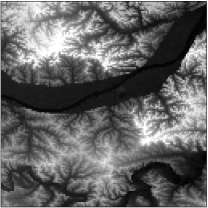
(a) True signal ${\bm{f}}\in{{\mathbb{R}}}^{128\times 128}$ such that $f_{i}\in{\left[{44,239}\right]}$. We measure $K=8192$ Gaussian random projections of this image.

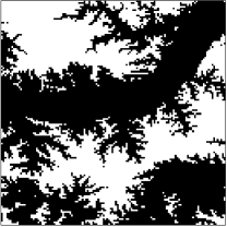
(b) Level set $S^{*}_{N}=\{i:f_{i}>125\}$ (white pixels) such that ${\left|{S^{*}_{N}}\right|}\approx 0.4285N$ where $N=128\times 128$.

Figure 2: Snapshots of the true signal and its desired level set.

We compare the performance of our method with the performances of the following approaches using the excess risk error metric defined in (3):

1. Thresholding method, where the estimate $\widehat{S}_{\gamma}$ is simply obtained by thresholding the proxy observations ${\bm{z}}$ at level $\gamma$; that is, $\widehat{S}_{\gamma}=\{i:z_{i}\geq\gamma\}$.

2. Risk-optimal thresholding method, where the estimate $\widehat{S}_{\widehat{\gamma}}$ is obtained by thresholding ${\bm{z}}$ at a level $\widehat{\gamma}$ that minimizes the excess risk; that is, $\widehat{S}_{\widehat{\gamma}}=\{i:z_{i}\geq\widehat{\gamma}\}$ where $\widehat{\gamma}=\mathop{\rm arg\,min}_{\gamma}{\varepsilon}_{N}{{\left({\widehat{S}_{\gamma},S^{*}_{N}}\right)}}$.

3. Non-iterative wavelet-based plug-in method, where the estimate $\widehat{S}_{w}$ is obtained by first estimating ${\bm{f}}$ from ${\bm{z}}$ using translation invariant wavelet denoising, and then thresholding the resulting estimate ${\bm{\widehat{f}}}$ at level $\gamma$; that is, $\widehat{S}_{w}=\{i:\widehat{f}_{i}\geq\gamma\}$. In these experiments we perform wavelet denoising using Daubechies-4 wavelets and soft thresholding, where the threshold is chosen to minimize the excess risk.

4. Total-variation (TV) based plug-in method, where the estimate $\widehat{S}_{TV}$ is obtained according to $\widehat{S}_{TV}={\left\{{i:\widehat{f}^{(TV)}_{i}\geq\gamma}\right\}}$. The estimate ${\bm{\widehat{f}}}^{(TV)}$ of the input image ${\bm{f}}$ is obtained from ${\bm{y}}$ by solving

   $${\bm{\widehat{f}}}^{(TV)}=\mathop{\rm arg\,min}_{{\bm{\widetilde{f}}}}{\left\|{{\bm{y}}-{\bm{A}}{\bm{\widetilde{f}}}}\right\|}_{2}^{2}+\tau{\left\|{{\bm{\widetilde{f}}}}\right\|}_{TV}$$

   where ${\left\|{{\bm{\widetilde{f}}}}\right\|}_{TV}$ is the total-variation norm of ${\bm{\widetilde{f}}}$, and $\tau$ is a user-defined parameter that balances the log-likelihood term and the regularization term. Algorithms such as the two-step iterative shrinkage and thresholding (TwIST) method provide a way to efficiently solve for the above optimization problem [twist]. In our experiments, $\tau$ is chosen to minimize the excess risk.

In these simulation experiments, we compute the excess risk clairvoyantly based on the knowledge of ${\bm{f}}$. We obtain the estimate $\widehat{S}$ using our projective level set estimator according to $\widehat{S}_{N}=\mathop{\rm arg\,min}_{{S}\in\mathcal{S}_{M}}\widehat{R}({S})+\tau{{{\rm pen}}}({S})$ with a scaling factor $\tau$, which is chosen to minimize ${\varepsilon}{{\left({\widehat{S}_{N},S^{*}_{N}}\right)}}$. In these experiments, we use $M=N$.

We evaluate the performance of all the competing algorithms discussed above, with and without projected mean subtraction discussed in Sec. 4. The number of observations used in these experiments is $K=N/2=8192$. Fig. 3(a) shows the proxy observations obtained without mean subtraction. Fig. 3(b) shows the level set estimate obtained by simply thresholding the proxy observations at level $\gamma$ and Fig. 3(c) shows the estimate obtained by performing the risk-optimal thresholding method. These results demonstrate that thresholding noisy, proxy observations results in several false positives and misses. Though the wavelet-based plug-in method yields better results in comparison, as shown in Fig. 3(d), the estimate is still severely oversmoothed and noisy. The estimate obtained using our projective level set estimator is shown in Fig. 3(e). This approach yields lower excess risk compared to the other three approaches discussed above, preserves some of the fine details, but still performs some oversmoothing. Fig. 3(f) shows the results obtained using the TV-based plug-in method. This method yields the best results compared to the other approaches and yields the smallest excess risk, at the expense of first estimating the signal. Fig. 3(g) plots excess risk as a function of the number of measurements $K<N=16384$ for all competing methods. These plots are obtained by averaging the results obtained over 200 different noise and projection matrix realizations.

Figs. 4(a) through 4(g) show the improvements in results obtained because of the projected mean subtraction. The improvements stem from the fact that the proxy measurements are less “noisy” after the projected mean subtraction. This subtraction operation lowers the excess risk of the estimates obtained using every method discussed above, except for the TV-based plug-in method, which performs very well in practice irrespective of mean subtraction. TV-based reconstruction is in general implemented using iterative algorithms where convergence is achieved if the mean squared error between estimates obtained in successive iterations does not change beyond a user-specified tolerance value. The TwIST algorithm used in our simulation study uses the proxy measurements to initialize the iterative process and stops iterating when convergence is achieved. As a result, only the number of iterations to achieve a specified convergence will change depending on the quality of the proxy observations and not the final estimate. This explains why the TV-based results are insensitive to projected mean subtraction.

The TV-based method seems to outperform our projective level set estimator since we evaluate the performance of these methods based solely on the excess risk and not on the computational resources required to achieve that excess risk. In that sense, this comparison is somewhat unfair. A more meaningful comparison would be to either evaluate the excess risk obtained within some unit time, or compare the time taken by different approaches to achieve a desired excess risk as the problem size $N$ changes. To make the comparison fair, we ran our projective level set estimator for different problem sizes, used $K\approx N/3$ observations to get our estimates, recorded the excess risk obtained in each case, and ran the TV-based plug-in method to achieve the same excess risk in each case. In other words, instead of using the conventional convergence strategy in TV-based reconstruction algorithm, we stop iterating if the excess risk is less than or equal to the one obtained using our method. We compare the computational time required for both these methods as a function of problem size. Figs. 5(a) and 5(b) show a $512\times 512$ image and its corresponding level set, respectively. Note that the image used in above experiments is a cropped version of the image in Fig. 5(a). We cropped this image in order to get images of different sizes. In particular, we used images of size $\ell\times\ell$ where $\ell=76,96,116,\ldots,376$. Fig. 5(c) shows the time-gap between these two methods to achieve similar excess risks, as a function of the number of pixels in the input image. These plots show that the computational time taken by TV-based plug-in method dramatically increases with problem size, where as the computation time required by our projective level set estimator increases much more gracefully with problem size.

Before concluding, it is also important to comment on the performance of our approach in relation to that of faster plug-in methods, such as those based on the SVD of ${\bm{A}}$. As noted in Sec. 2.1, we do not expect such methods to perform well in the underdetermined ($K<N$) setting for reasons outlined earlier. We have also verified this intuition through numerical experiments (not fully reported here for space reasons). Consider, for example, estimating the level set in Fig. 2(b) by thresholding either TSVD or Tikhonov regularized solution for the case of $K\approx N/2$. In this setting, the excess-risks obtained using TSVD and Tikhonov regularization-based plug-in methods are $14.26$ and $14.31$ respectively, where as the excess-risk using our proposed method is $3.593$. This rather poor performance of SVD-based plug-in methods should not be too surprising. Such methods operate on the assumption that signals lie near a subspace, but a union-of-subspaces model is known to be a better model for real-world signals [Lu.Do.ITSP2008]. In contrast to SVD-based approaches, our method performs better since the family ${S}_{m}$ over which we search for an estimate of the level set can be construed as a union-of-subspaces, with each subspace in the union being formed by a set of indices corresponding to dyadic, tree-based basis functions.

In conclusion, the experimental results indicate that estimating the underlying signal using TV regularization-based plug-in methods yields more accurate level set estimates compared to the ones obtained using our projective level set estimator. However, the real strengths of our method are two-fold. First, we can reliably perform real-time level set estimation compared to plug-in methods as shown by the time-gap versus problem size plot in Fig. 5(c). Second, we can use our level set estimate to discard regions where the levels of interest are not present and design adaptive measurement schemes to hone-in on the regions of interest. Such an adaptive measurement scheme is especially helpful in very high-dimensional settings where the cost of collecting measurements and performing reconstruction tends to be extremely high.

(a) Proxy observations

(a) Proxy observations after projected mean subtraction

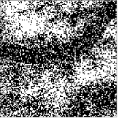
(b) Estimate obtained using the thresholding method; ${\varepsilon}_{N}=8.562$

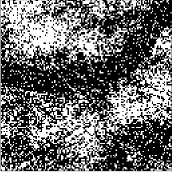
(c) Estimate obtained using the risk-optimal thresholding method; ${\varepsilon}_{N}=8.231$

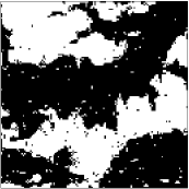
(d) Estimate obtained using the wavelet-based method; ${\varepsilon}_{N}=2.393$

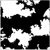
(e) Estimate obtained using the projective level set estimator; ${\varepsilon}_{N}=1.924$

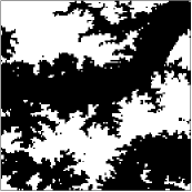
(f) Estimate obtained using the TV-based plug-in estimator; ${\varepsilon}_{N}=0.5593$

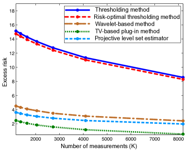
(g) Plot of excess risk as a function of $K<N=16384$ after performing mean subtraction.

Figure 4: Snapshots of the simulation results obtained (after performing projected mean subtraction) from observations of the form in (1).

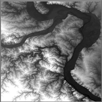
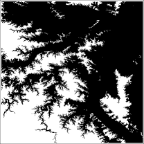
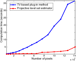
(a)	(b)	(c)

Figure 5: Comparison of the computation times of TV-based plug-in method and our projective level set estimator. (a) True signal ${\bm{f}}\in{{\mathbb{R}}}^{512^{2}}$ such that $f_{i}\in{\left[{0,239}\right]}$, (b) level set $S^{*}_{N}=\{i:f_{i}>125\}$, and (c) a plot of computation time as a function of problem size to approximately achieve the same excess risk. Images of different sizes ($76\times 76$ to $376\times 376$) cropped from (a) were used in this experiment. The plots in (c) indicate that the time it takes for the TV-based plug-in method to achieve the same excess risk obtained by the projective level set estimator increases dramatically with problem size.

8 Conclusion

This work proposes a theoretically sound and computationally efficient tree-based approach for extracting level sets of a function from projection measurements without reconstructing the underlying function. The simulation results presented in Sec. 7 suggest that the proposed method may facilitate fast and accurate level set estimates from tomographic projections in medical imaging, Fourier projections in interferometry, or coded projections in compressive optical systems. One of the key advantages of our approach is that many of the operations on the proxy data are easily parallelizable. For instance, in problems where the domain of the signal of interest is very large, we can compute the proxy observations, partition the proxy data into different patches, run our estimation algorithm on each patch separately and merge the results to identify the regions that correspond to the level set. In applications such as medical imaging, the time saved by collecting fewer projection measurements and parallelization can be significant and crucial.

Empirically, the accuracy of the projective level set estimate is comparable to that of a similar scheme based on wavelet thresholding or an iterative method with TV regularization. Currently, however, there is no theoretical support for these alternatives. Recent work studying the performance of so-called “analysis regularization” [vaiter2011robust, giryes2010rip] may lead to an improved understanding of theoretical performance bounds for the TV approach, but as we show here this iterative solution requires significantly more computational resources. Our approach is much more similar in spirit to the wavelet-based approach, and the theoretical techniques employed in our analysis may lead to an improved understanding of this and other fast, non-iterative approaches. Furthermore, adaptive sampling schemes such as the one discussed in [haupt2009compressive] suggest a potential extension of our method. Specifically, [haupt2009compressive] proposes collecting noisy measurements of a sparse signal, estimating its support and collecting more measurements based on the estimated support to adaptively focus the computational resources on regions of interest. The underlying assumption in such “distilled sensing” [haupt2009distilled] schemes is sparsity. Since our level set estimation method offers a way to estimate the level set of a function without requiring sparsity, we expect it to facilitate the development of new adaptive sampling routines that perform better than the ones proposed in earlier works.

References

- [1] Special Issue on Compressive Sampling, IEEE Signal Processing Magazine, 25 (2008).
- [2] I. Ayed, A. Mitiche, and Z. Belhadj, Multiregion level-set partitioning of synthetic aperture radar images, IEEE Transactions on Pattern Analysis and Machine Intelligence, (2005), pp. 793–800.
- [3] W. U. Bajwa, R. Calderbank, and S. Jafarpour, Why Gabor frames? Two fundamental measures of coherence and their role in model selection, J. Commun. Netw., (2010), pp. 289–307.
- [4] W. U. Bajwa, R. Calderbank, and D. G. Mixon, Two are better than one: Fundamental parameters of frame coherence, Appl. Comput. Harmon. Anal., 33 (2012), pp. 58–78.
- [5] J. Bioucas-Dias and M. Figueiredo, A New TwIST: Two-Step Iterative Shrinkage/Thresholding Algorithms for Image Restoration, IEEE Transactions on Image Processing, 16 (2007), pp. 2992 –3004.
- [6] T. Blumensath and M. Davies, Iterative hard thresholding for compressed sensing, Applied and Computational Harmonic Analysis, 27 (2009), pp. 265–274.
- [7] E. Candès, J. Romberg, and T. Tao, Robust uncertainty principles: Exact signal reconstruction from highly incomplete frequency information, IEEE Transactions on Information Theory, 52 (2006), pp. 489 – 509.
- [8] E. Candés and T. Tao, Near optimal signal recovery from random projections: Universal encoding strategies, IEEE Transactions on Information Theory, 52 (2006), pp. 5406–5425.
- [9] S. Chen and D. Donoho, Basis pursuit, in Signals, Systems and Computers, 1994. 1994 Conference Record of the Twenty-Eighth Asilomar Conference on, vol. 1, Oct-2 Nov 1994, pp. 41–44 vol.1.
- [10] A. Cuevas, W. González-Manteiga, and A. Rodríguez-Casal, Plug-in estimation of general level sets, Australian & New Zealand Journal of Statistics, 48 (2006), pp. 7–19.
- [11] D. Donoho, Compressed sensing, IEEE Transactions on Information Theory, 52 (2006), pp. 1289–1306.
- [12] D. Donoho and I. Johnstone, Ideal spatial adaptation by wavelet shrinkage, Biometrika, 81 (1994), pp. 425–455.
- [13] M. F. Duarte and Y. C. Eldar, Structured compressed sensing: From theory to applications, IEEE Trans. Signal Processing, 59 (2011), pp. 4053–4085.
- [14] A. Fletcher, S. Rangan, and V. Goyal, Necessary and sufficient conditions for sparsity pattern recovery, IEEE Transactions on Information Theory, (2009), pp. 5758–5772.
- [15] C. Genovese, J. Jin, and L. Wasserman, Revisiting marginal regression, Arxiv preprint arXiv:0911.4080, (2009).
- [16] R. Giryes and M. Elad, RIP-based near-oracle performance guarantees for SP, CoSaMP, and IHT, IEEE Trans. Signal Processing, 60 (2012), pp. 1465–1468.
- [17] Z. Harmany, R. Willett, A. Singh, and R. Nowak, Controlling the error in FMRI: Hypothesis testing or set estimation?, in 5th IEEE International Symposium on Biomedical Imaging: From Nano to Macro, IEEE, 2008, pp. 552–555.
- [18] J. Haupt, R. Baraniuk, R. Castro, and R. Nowak, Compressive distilled sensing: Sparse recovery using adaptivity in compressive measurements, in Forty-Third Asilomar Conference on Signals, Systems and Computers, IEEE, 2009, pp. 1551–1555.
- [19] J. Haupt, R. Castro, and R. Nowak, Distilled sensing: Selective sampling for sparse signal recovery, in Proc. 12th International Conference on Artificial Intelligence and Statistics (AISTATS), Citeseer, 2009, pp. 216–223.
- [20] G. Herman, Image Reconstruction from Projections, The Fundamentals of Computerized Tomography, New York Academic Press, 1980.
- [21] W. Hoeffding, Probability inequalities for sums of bounded random variables, J. Amer. Statist. Assoc., 58 (1963), pp. 713–721.
- [22] D. Huang, E. A. Swanson, C. P. Lin, J. S. Schuman, W. G. Stinson, W. Chang, M. R. Hee, T. Flotte, K. Gregory, C. A. Puliafito, et al., Optical coherence tomography, Science, 254 (1991), pp. 1178–1181.
- [23] W. Jang and M. Hendry, Cluster analysis of massive datasets in astronomy, Statistics and Computing, 17 (2007), pp. 253–262.
- [24] J. Kaipio and E. Somersalo, Statistical and Computational Inverse Problems, Springer, New York, NY, 2005.
- [25] K. Krishnamurthy, W. Bajwa, R. Willett, and R. Calderbank, Fast level set estimation from projection measurements, in Statistical Signal Processing Workshop (SSP), 2011 IEEE, IEEE, 2011, pp. 585–588.
- [26] A. Kyrieleis, V. Titarenko, M. Ibison, T. Connolley, and P. Withers, Region-of-interest tomography using filtered backprojection: Assessing the practical limits, Journal of Microscopy, (2010).
- [27] B. Laurent and P. Massart, Adaptive estimation of a quadratic functional by model selection, Annals of Statistics, (2000), pp. 1302–1338.
- [28] R. M. Lewitt, Processing of incomplete measurement data in computed tomography, Medical physics, 6 (1979), p. 412.
- [29] C. Li, C. Xu, K. Konwar, and M. Fox, Fast distance preserving level set evolution for medical image segmentation, in Proc. 9th Intl. Conf. Control, Automation, Robotics and Vision, IEEE, 2006, pp. 1–7.
- [30] Y. Lu and M. Do, A theory for sampling signals from a union of subspaces, IEEE Trans. Signal Processing, 56 (2008), pp. 2334–2345.
- [31] J. Ma, Iterative region of interest reconstruction in emission tomography, in IEEE International Symposium on Biomedical Imaging: From Nano to Macro,, April 2010, pp. 604 –607.
- [32] C. Maaß, M. Knaup, and M. Kachelrieß, New approaches to region of interest computed tomography, Medical Physics, 38 (2011), p. 2868.
- [33] R. Marques, F. De Medeiros, and D. Ushizima, Target detection in SAR images based on a level set approach, Systems, Man, and Cybernetics, Part C: Applications and Reviews, IEEE Transactions on, 39 (2009), pp. 214–222.
- [34] D. Mason and W. Polonik, Asymptotic normality of plug-in level set estimates, The Annals of Applied Probability, 19 (2009), pp. 1108–1142.
- [35] A. Moreno, Total error in a plug-in estimator of level sets, Statistics and Econometrics Working Papers, (2003).
- [36] R. Puetter, T. Gosnell, and A. Yahil, Digital image reconstruction: Deblurring and denoising, Annual Reviews on Astronomy and Astrophysics, 43 (2005), pp. 139–194.
- [37] P. Rigollet and R. Vert, Fast rates for plug-in estimators of density level sets, Bernoulli, 15 (2009), pp. 1154–1178.
- [38] P. Rosen, S. Hensley, I. Joughin, F. Li, S. Madsen, E. Rodriguez, and R. Goldstein, Synthetic aperture radar interferometry, Proceedings of the IEEE, 88 (2000), pp. 333–382.
- [39] M. Rudelson, Lecture notes on non-asymptotic theory of random matrices, arXiv preprint arXiv:1301.2382, (2013).
- [40] L. I. Rudin, S. Osher, and E. Fatemi, Nonlinear total variation based noise removal algorithms, Physica D: Nonlinear Phenomena, 60 (1992), pp. 259–268.
- [41] C. Scott and M. Davenport, Regression level set estimation via cost-sensitive classification, IEEE Transactions on Signal Processing, 55 (2007), pp. 2752–2757.
- [42] C. Scott and R. Nowak, Learning minimum volume sets, Journal of Machine Learning Research, 7 (2006), pp. 665–704.
- [43] C. Scott and R. Nowak, Minimax-optimal classification with dyadic decision trees, IEEE Transactions on Information Theory, 52 (2006), pp. 1335–1353.
- [44] A. Singh, C. Scott, and R. Nowak, Adaptive Hausdorff estimation of density level sets, The Annals of Statistics, 37 (2009), pp. 2760–2782.
- [45] D. Takhar, J. Laska, M. Wakin, M. Duarte, D. Baron, S. Sarvotham, K. Kelly, and R. Baraniuk, A new compressive imaging camera architecture using optical-domain compression, in SPIE, vol. 6065, 2006.
- [46] R. Tibshirani, Regression shrinkage and selection via the lasso, Journal of the Royal Statistical Society. Series B (Methodological), (1996), pp. 267–288.
- [47] J. Tropp and A. Gilbert, Signal recovery from random measurements via orthogonal matching pursuit, Information Theory, IEEE Transactions on, 53 (2007), pp. 4655 –4666.
- [48] A. Tsybakov, On nonparametric estimation of density level sets, Annals of Statistics, 25 (1997), pp. 948–969.
- [49] S. Vaiter, G. Peyré, C. Dossal, and J. Fadili, Robust sparse analysis regularization, Arxiv preprint arXiv:1109.6222, (2011).
- [50] V. Vapnik, The nature of statistical learning theory, Springer Verlag, 2000.
- [51] R. Vershynin, Norm of a random matrix. Lecture notes on Non-asymptotic theory of random matrices, 2006-2007.
- [52] Y. Wang, J. Yang, W. Yin, and Y. Zhang, A new alternating minimization algorithm for total variation image reconstruction, SIAM Journal on Imaging Sciences, 1 (2008), pp. 248–272.
- [53] R. Willett and R. Nowak, Minimax optimal level set estimation, IEEE Transactions on Image Processing, (2007), pp. 2965–2979.
- [54] Y. Yang, Minimax nonparametric classification-Part I: Rates of convergence, IEEE. Transactions on Information Theory, 45 (1979), pp. 2271–2284.