The Impact of Frequency Standards on Coherence in VLBI at the Highest Frequencies

Abstract

We have carried out full imaging simulation studies to explore the impact of frequency standards in millimeter and sub-millimeter Very Long Baseline Interferometry (VLBI), focusing on the coherence time and sensitivity. In particular, we compare the performance of the H-maser, traditionally used in VLBI, to that of ultra-stable cryocooled sapphire oscillators over a range of observing frequencies, weather conditions and analysis strategies. Our simulations show that at the highest frequencies, the losses induced by H-maser instabilities are comparable to those from high quality tropospheric conditions. We find significant benefits in replacing H-masers with cryocooled sapphire oscillator based frequency references in VLBI observations at frequencies above 175 GHz in sites which have the best weather conditions; at 350 GHz we estimate a 20-40% increase in sensitivity, over that obtained when the sites have H-masers, for coherence losses of 20-10%, respectively. Maximum benefits are to be expected by using colocated Water Vapour Radiometers for atmospheric correction. In this case, we estimate a 60-120% increase in sensitivity over the H-maser at 350 GHz.

1 Introduction

Pushing Very Long Baseline Interferometry (VLBI) observations to higher frequencies is a desirable approach to increase angular resolution and to target new and unique fields of science investigation. Nevertheless, the observations become increasingly challenging as the wavelengths get shorter. VLBI at millimeter and sub-millimeter wavelengths (hereafter mm-VLBI) suffer from low sensitivity which makes operations extremely difficult and dramatically restrict the scope of application. Thus mm-VLBI observations have been very limited. While wider bandwidths and increased recording rates will help alleviate the problems, the major breakthrough to improve sensitivity will come from directly addressing the causes. The sensitivity issues have their origin in the large coherence losses induced by the fast phase fluctuations imposed on the astronomical signal, which arise from atmospheric propagation of the radio waves and instrumental noise contributions, such as from the frequency standards (Thompson et al., 2007). These fast fluctuations impose short coherence times, which in turn increases the minimum detectable flux. To a lesser extent, the attenuation of the signal from atmospheric transmission also contributes. Moreover, in the high frequency regime the sensitivity of radio telescopes is reduced, the receiver noise is increased, and the intrinsic source strength is generally lower.

The reason for the atmospheric propagation issues lies in the variations in its refractive index, mainly due to inhomogeneities in the distribution of tropospheric water vapour in the turbulent atmosphere. These variations result in changes in the electrical path length through the atmosphere, which introduces phase fluctuation errors on spatio-temporal scales in the observed phase of the astronomical signal, degrading the sensitivity by reducing the coherence time. The fractional frequency stability contribution of a typical atmosphere to the received signal has been determined to have an Allan Standard Deviation (ADEV) of $\sim$10^-13s/s up to 100 seconds (Rogers et al., 1984; Rogers & Moran, 1981). Given the non dispersive nature of the troposphere, the induced temporal phase fluctuations scale linearly with observing frequency. Hence, to mitigate the fundamental limitation imposed by atmospheric propagation, it is essential to select a site with exceptionally stable and transparent atmospheric conditions; dry high altitude sites. In addition, the potential of using inferred corrections estimated from measurements of sky brightness temperatures using co-located Water Vapour Radiometers (WVR) is a long term on-going effort. Currently, the ALMA (Atacama Large Millimeter Array ) project is developing state-of-the-art WVRs to compensate for tropospheric fluctuations. Preliminary observations with these instruments show promising performance, with progress towards their nominal specification (98% compensation of the fluctuations) (nic_wvn). WVR’s application to VLBI holds the promise of a significant breakthrough in dealing with current tropospheric limitations (Honma, 2012; Matsushita et al., 2012).

In mm-VLBI, the other dominant error contribution to the residual phase fluctuations arises from the instabilities of the frequency standard traditionally used in VLBI, the Hydrogen (H)-maser. The aim of the work presented here is to assess the benefits of replacing a H-maser with an ultra-stable cryoCooled Sapphire Oscillator (CSO), whose stability is more than 1 order of magnitude better at the short timescales of interest in this field, as an option for mm-VLBI.

Previous studies of Doeleman and collaborators investigated a liquid helium cooled Sapphire Oscillator, along with the estimated performance of a 10 MHz synthesized signal, and showed a moderate benefit at 350 GHz. The next generation of CSOs has become a very robust, low maintenance, long term operational alternative to the H-maser as an ultra-stable frequency standard, now that the device operates with a low vibration pulse-tube cryocooler (Wang & Hartnett, 2010; Hartnett et al., 2010; Hartnett & Nand, 2010). The CSO’s performance is well established and the measured frequency stability for both short and long term timescales is better than that achieved with the liquid helium cooled version (Doeleman et al., 2011; Nand et al., 2011; Hartnett et al., 2012). Additionally, the new version generates a 100-MHz synthesized signal which has significantly better performance (Nand et al., 2011). The Doeleman study was completed before these improvements to the CSO were implemented and were largely analytic, being based on the standard expressions for coherence. We have completed full imaging simulations which are much more sensitive to the cumulative effects of different error sources. Furthermore, only a limited analysis of the effect of WVR was included in Doeleman’s studies, which we have considerably advanced.

In this paper we present the results from full imaging simulations to explore the performance of VLBI observations using a H-maser versus a CSO under a variety of conditions, to answer the questions of whether, and under which circumstances, the CSO could be expected to provide benefits over a H-maser. Our simulation studies also explore the potential of various analysis strategies to enhance the coherence time, in particular using simultaneous dual frequency observations and the use of collocated WVRs to correct for tropospheric fluctuations.

This is the first step in the process to fully test the application of ultra-stable CSOs to facilitate mm-VLBI observations. The results obtained from these simulation studies will serve as a guideline for an empirical demonstration with actual observations. In this paper, a description of the simulation procedure is presented in Section 2. The results are presented in Section 3, and discussion of results in Section 4.

2 The Method

In this section we describe the procedure followed in our full imaging simulation studies to explore the benefits of replacing a H-maser with a CSO, along with the potential of different analysis strategies, in mm-VLBI. First, we used an updated version of ARIS (Asaki et al., 2007) to generate the synthetic datasets which replicate the interferometric visibilities obtained from a correlator for a given observing configuration, i.e. coordinates of the telescopes and the celestial target, observing frequencies, bandwidth, atmospheric conditions, etc. ARIS is a versatile software tool which includes complete two dimensional geometric and atmospheric phase screen models, and has been used in previous simulation studies for ground and space VLBI (Asaki et al., 2007; Rioja et al., 2011). We have found it reproduces the results from actual observations extremely well (Asaki et al., 2010). Among the functionalities added in order to carry out this project are the options to incorporate the noise contributions from the station frequency standards (i.e. clock errors), for both H-masers and CSOs, to select ALMA-site type weather conditions (i.e. Very Good), and to generate WVR corrected tropospheres, in simulations at frequencies up to 350 GHz.

Table 1 lists the parameter space explored in our simulations. These comprise of observations at frequencies between 86 to 350 GHz, using H-maser and CSO clocks, for a range of weather conditions classified as: Very Good, Good, Typical and Poor, using different telescope networks, and realistic errors for the model parameters. We also explore the case of having WVR-corrected atmospheres. These simulations are mainly concerned with the relative impact of tropospheric and clock instabilities. Therefore, in order to avoid bias effects introduced by observations of weak sources, the simulations were all run with strong signals and are thermal noise free.

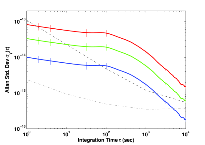
Figure 1: Plot of the Allan Standard Deviations for the atmospheres and the frequency standards from ARIS. Shown in solid lines are the Good (in red, upper most), the Very Good (in green) and the WVR-corrected (blue, lowest) atmospheres. The dash line is the ADEV for a KVARZ H-maser and the dot-dash for the CSO-100 MHz. The atmosphere values are extracted from the mean of repeated runs of independent model generation in ARIS, with error bars marking the $\pm$1-$\sigma$ standard deviation from the mean.

ARIS implements the clock and tropospheric fluctuations by generating a time series of random values which are statistical realizations of models in the code. The functional forms of the time standard noise used are polynomial expansions of the ADEV which follow Nand et al. (2011) and represent the observed CSO behaviour and the quoted behaviour of the Russian KVARZ H-maser. The simulated fluctuations of the atmospheric path can be generated for a choice of four weather conditions, i.e. Very Good (V), Good (G), Typical (T) and Poor (P), adjusting the modified coefficient of the spatial structure function of the troposphere to values 0.5, 1, 2 and $4\times 10^{-7}m^{-1/3}$, respectively, with the assumption of Kolmogorov turbulence (Asaki et al., 2007; Beasley & Conway, 1995). For example, the “Very Good” weather corresponds to an rms excess path length of 100 microns for a 100-m baseline (ca. 50-percentile tropospheric condition at Chajnantor Observatory site (Chile)) (Asaki et al., 2005). Larger fluctuations correspond to more unstable tropospheric conditions. The option for WVR phase correction (W) implemented in ARIS matches empirical results from ALMA commissioning and science verification observations, with ALMA WVRs at 183 GHz (for 600-m baselines) (Matsushita et al., 2012), which typically result in the rms phase reduced to 30-40%. Hence, the W option reduces the rms phase of Very Good weather by a factor of 3, keeping the assumption of Kolmogorov turbulence and adds a WVR path length measurement Gaussian noise to each antenna (1-$\sigma$ equal to 4 microns, for 10 seconds average data).

Figure 1 shows the model frequency stability, characterized in terms of the ADEV, for the clock (for CSO and H-maser) and atmospheric (W, V, and G) errors with ARIS. We have confirmed that the behaviour of the atmospheric models in ARIS are consistent with known approximations and published results. The driver for our detailed examination was that the coherence times we derived appeared to be in excess of the established limits. These resolved themselves into differences in the definition of loss limits deemed acceptable or in the procedures followed. Different authors use different cutoffs for the coherence losses, and these lead naturally to different coherence times. We have used the maximal value for the allowed phase rms of 1 radian, corresponding to an approximately 40% signal loss, following the discussions in Thompson et al. (2007) (Eq. 9.119). On the other hand, setting limits of 10% signal loss translate into a phase rms of 0.4 radians. We have calculated the coherence factor at 86 GHz with Eq. 7 of Nand et al. (2011) assuming the standard ADEV of ‘Good’ tropospheric conditions. We find identical losses as a function of integration time as those derived from the ARIS model atmospheres. The matching coherence times were obtained both by direct averaging, and the similar approach of phase-only calibration (with CALIB in AIPS (Greisen, 2003)).

We have performed all our simulations in the strong signal domain, assuming that the next generation telescopes making up the Event Horizon Telescope (Doeleman, 2010) will be highly sensitive with excellent performance and wide bandwidths. Therefore we used a 10 Jy model source and no thermal noise was added. In the strong signal domain one can use coherent methods (i.e. fringe finding for delays and rates as well as phase) and direct imaging, as opposed to forming closure products with incoherently derived delays and model fitting the data. This allows us to extend the coherence time well beyond the values obtained following the methods above. As the ADEV of our model atmospheres follow those of observed atmospheres, we are confident that fringe-fitted real data will show similar behaviour. We find our simulated results compare with the coherence quoted in papers on VLBI observations at 86 GHz (e.g. Middelberg et al. (2005)).

The simulated datasets comprise all combinations of tropospheric conditions and clock types for observations at each frequency (i.e. 86, 175 and 350 GHz), and for simultaneous dual-frequency observations (i.e. 43/86GHz; 87/175GHz; 175/350GHz). In addition, datasets with a single noise contribution, either atmospheric or clock errors, have been used to explore the individual signatures and their dependence on observing frequency. Table 2 summarizes the 5 simulation cases presented in this paper. The output of ARIS are standard uv-FITS files with corrupted visibilities, as described in Table 2 for each configuration, ready for processing with AIPS.

Each synthetic dataset was analysed using calibration and imaging procedures in AIPS to produce images. The analysis was carried out following different calibration strategies, listed in Table 2:
1) standard VLBI self-calibration procedures for the analysis of single frequency datasets (i.e. Cases 1,2,3). For each dataset, we repeated the analysis with different FRING solution intervals in the range from 0.1 to 6 minutes to explore coherence losses;
2) frequency phase transfer calibration (FPT) procedures (Rioja & Dodson, 2011) for the simultaneous dual-frequency datasets. That is, the high frequency data are calibrated using the scaled self-calibration estimates from the lower frequency (i.e. Case 4). The FPT calibration compensates all non-dispersive errors, but long timescale ionospheric errors, and in general any dispersive error, still remains.
3) a hybrid calibration with FPT and self-calibration (i.e. Case 5). That is, same as 2) combined with a further cycle of self-calibration with a much longer solution interval in FRING to correct for the dispersive terms.

In all cases, the calibrated complex visibility samples were Fourier transformed, and deconvolved, using standard imaging procedures with the AIPS task IMAGR, to produce an image. And finally, the map peak flux was measured using the AIPS task JMFIT. The fractional flux recovery (FFR) quantity, defined as the ratio between the peak flux in the map divided by the source model flux (in ARIS), was used as the figure of merit to evaluate and compare the coherence losses for each configuration. The values presented here are the mean and rms of the FFR measured from 5 simulation runs for each configuration, each with independently generated noise time series for the model errors in ARIS. Larger values of the FFR correspond to smaller coherence losses, which in turn lead to higher sensitivity. This comparison is ultimately used to assess the benefits of replacing the H-maser with CSOs.

Table 1: Parameter space of our simulations with ARIS

GEOMETRY(1):
Array	VLBA
Source	Compact and Strong
PROPAGATION MEDIA(2):
Ionosphere	Error: 6 TECU
	Fluctuations: Nominal
Troposphere	Error: 3 cm
	Fluctuations: WVR-corrected, V, G, T, P
FREQUENCY STANDARD:	H-maser, CSO-100 MHz
OBSERVING FREQUENCY:
Single Frequency	86, 175, 350 GHz
Dual Frequency	43/86 GHz, 87/175 GHz, 175/350 GHz

(1): VLBA: Very Long Baseline Array. The telescope and source coordinates are simply used to generate the tracks, i.e. sampling of the uv-plane.
(2): See Asaki et al. (2007) for detailed information.

Table 2: Description of the simulation study cases presented in this paper, based on the nature of the error contributions to the synthetic datasets generated with ARIS, and the data analysis procedure with AIPS.

		Simulation Cases
		Case 1	Case 2	Case 3	Case 4	Case 5
ERRORS
	GEO errors			X
	CLOCK noise
	H-maser; CSO	X		X	X	X
	ATM noise
	V;G;T;P		X	X	X	X
	WVR-corrected (W)		X	X
	Obs. FRQ (GHz)	86	86	86	43/86	43/86
		175	175	175	87/175	87/175
		350	350	350	175/350	175/350
ANALYSIS
	SC1	X	X	X
	FPT2				X
	FPT + SC3					X

(1): Self-Calibration
(2): Frequency Phase Transfer, using dual-frequency observations.
(3): A combination of the two above.

3 Results

The final products of our simulations are images, and the FFR values measured from them. We use FFR as the figure of merit to compare performance, that is the associated coherence losses, for the simulated configurations. In this section we present the results from our simulations following a classification similar to that shown in Table 2. The interpretation of these results in terms of sensitivity is addressed in section 4.

3.1 Case 1: Clock Errors Only (Atmosphere Noise-Free)

Figure 2 shows the FFR values from simulations with clock noise only at 86, 175 and 350 GHz, for a range of integration times in the self-calibration analysis with AIPS. The coherence losses associated with the H-maser instabilities significantly increase with the observing frequency, and for a given frequency at longer integration times. In comparison, the coherence losses from the CSO are negligible, at all frequencies and for the same range of integration times. Our simulations with clock noise only show that the instabilities from a H-maser result in $\sim 10\%$ losses in 0.5-1 minutes at 350 GHz, and $\sim 20\%$ losses in $\sim 2$ minutes. The corresponding losses for the same integration times in the case of the CSO are $\leq 0.5\%$.

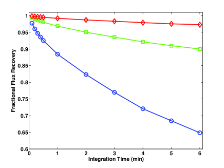
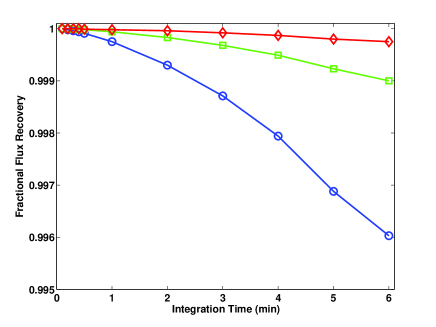
Figure 2: Left: Coherence losses, plotted as the Fractional Flux Recovered, introduced by the H-maser clock instabilities as a function of the integration time, in observations at 86 (red diamond), 175 (green square) and 350 (blue circle) GHz; Right: same, for CSO-100 MHz.

3.2 Case 2: Atmospheric Errors Only (Clock Noise-Free)

Figure 3 shows the results from simulations involving only atmospheric instabilities (i.e. the clock-noise free case). At a given frequency, the FFR decreases with increasing integration times, and with worsening weather conditions, being highest for V and lowest for P for each integration time value, as expected from increasing signal coherence losses. For example, at 350 GHz these simulations result in peak flux losses of $\sim 20\%$ on timescales of $\sim 1$ minute, under V weather conditions, and $\sim 0.5$, 0.2 and 0.1 minutes with G, T and P weather conditions, respectively. Also, for a given weather and integration time, the coherence losses are increasingly large at higher frequencies. This is in agreement with the well recognized importance of selecting sites with excellent weather conditions for VLBI at the highest frequencies. Best results at all frequencies are found when using WVR-corrected atmospheres; for example, at 350 GHz, these simulations result in peak flux losses of $\sim 20\%$ on much longer timescales of $\sim 5$ minutes.

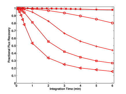
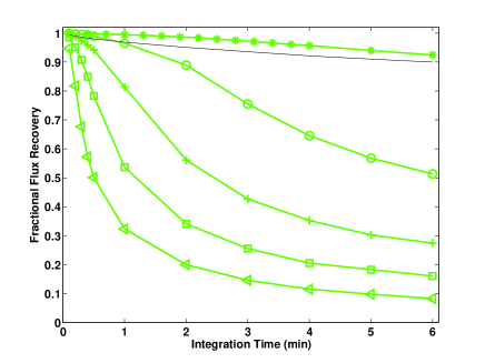
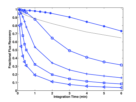
Figure 3: Atmospheric-induced coherence losses, plotted as the Fractional Flux Recovered, versus integration time estimated for a range of weather conditions (V (circle), G (plus), T (square), P (diamond)) and for WVR-corrected atmospheres, W (star), at 86 (upper left), 175 (upper right) and 350 (lower left) GHz. At each frequency, the sequence of lines starting from the uppermost correspond to W,V,G,T,P weather conditions. The rms errors are smaller than the symbol size. For illustration, a light black line indicates the losses due entirely to a H-maser (shown in Figure 2).

3.3 Comparison of Case 1 and Case 2

Figure 4 shows the superimposed results from the simulation cases above: with only clocks and with only tropospheric noise contributions. The point at which the losses from the H-maser and the tropospheric instabilities are equal increases in significance with the observing frequency and the quality of weather conditions. For sufficiently short timescales ($<$1 minute) the H-maser losses dominate under V weather conditions, with contributions of up to 15% at 350 GHz, but are negligible at 86 and 175 GHz; these timescales are much longer ($>$6 minutes) for WVR-corrected atmospheres, with H-maser losses up to $>$10% and 35%, at 175 and 350 GHz, respectively. Note that the coherence losses with the CSO-only are negligible ($<0.5\%$) in all cases, and have not been included in the plots.

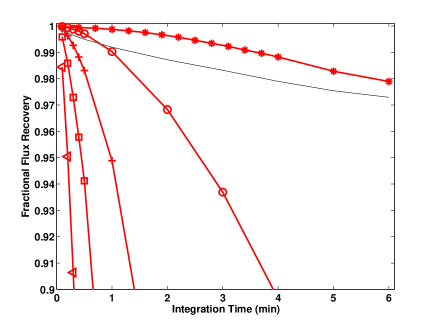
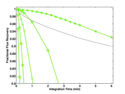
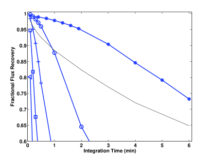
Figure 4: Zoomed versions of Figure 3, focusing in on the short timescales at which the H-maser losses are greater than, or a significant fraction of, the atmospheric contributions. As in Figure 3, the atmospheric-induced coherence losses (the Fractional Flux Recovered) estimated for a range of weather conditions (V,G,T,P) and for WVR-corrected atmospheres (W), are plotted versus integration time at 86 (upper left), 175 (upper right) and 350 (lower left) GHz. At each frequency, the sequence of lines starting from the uppermost correspond to W,V,G,T,P weather conditions. A light black line indicates the losses due entirely to a H-maser.

3.4 Case 3: Clock and Atmospheric Noise

In complete simulations, with joint tropospheric and clock instabilities, the estimated losses are the combination of the corresponding individual ones. Hence, the significance of the H-maser noise is expected to increase at higher frequencies and with better weather conditions, while the CSO noise remains negligible in all circumstances.

Figures 5, 6 and 7 show the results from realistic simulations with clock and atmospheric instabilities. Figure 5 shows superimposed the FFR measured for the case of WVR-corrected atmospheres both with a H-maser and with a CSO at all frequencies. Figures 6 and 7 are equivalent to Figure 5, but for V and G weather conditions, respectively. Additionally, Figures 5 to 7 include the fractional change between the FFR estimated from both simulation cases, with the H-maser and the CSO, at the corresponding frequency and weather conditions, as a function of integration time.

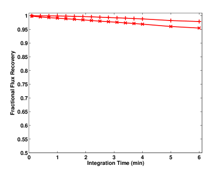
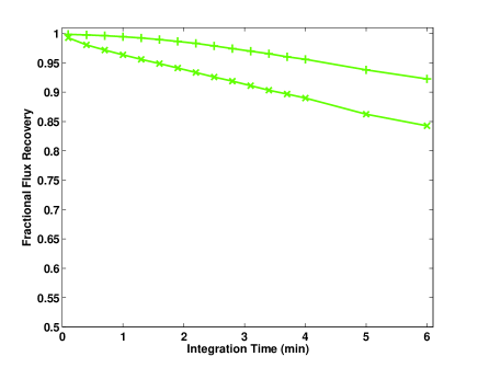
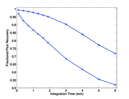
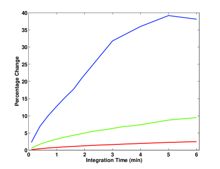
Figure 5: The fractional flux recovered with WVR-corrected tropospheric atmospheric models plus clock (CSO ‘+’; H-maser ‘x’) instabilities, versus integration time, at 86 (red, upper left), 175 (green, upper right) and 350 (blue, lower left) GHz. The rms errors are smaller than the symbol size. Additionally, the lower right plot shows the fractional increase in coherence loss when using a H-maser in place of a CSO, versus integration time, for the three frequencies. The frequencies run from the highest at the top to the lowest at the bottom.

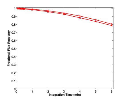
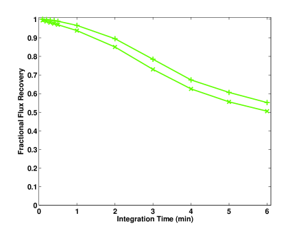
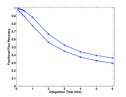
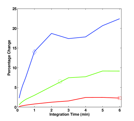
Figure 6: The fractional flux recovered with Very Good (V) tropospheric atmospheric models plus clock (CSO ‘+’; H-maser ‘x’) instabilities, versus integration time, at 86 (red, upper left), 175 (green, upper right) and 350 (blue, lower left) GHz. The rms errors are smaller than the symbol size. Additionally, the lower right plot shows the fractional increase in coherence loss when using a H-maser in place of a CSO, versus integration time, for the three frequencies as in Figure 5. For each frequency a symbol (a diamond for 350 GHz, a circle for 175 GHz and a square for 86 GHz) marks the point corresponding to losses of 20% in the H-maser simulations.

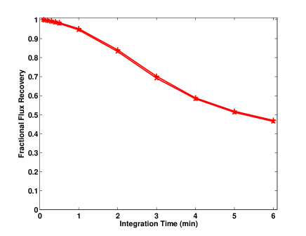
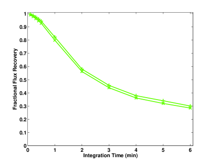
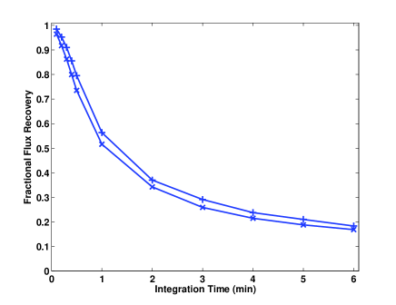
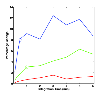
Figure 7: The fractional flux recovered with Good (G) tropospheric atmospheric models plus clock (CSO ‘+’; H-maser ‘x’) instabilities, versus integration time, at 86 (red, upper left), 175 (green, upper right) and 350 (blue, lower left) GHz. The rms errors are smaller than the symbol size. Additionally, the lower right plot shows the fractional increase in coherence loss when using a H-maser in place of a CSO, versus integration time, for the three frequencies as in Figure 5. For each frequency a symbol (a diamond for 350 GHz, a circle for 175 GHz and a square for 86 GHz) marks the point corresponding to losses of 20% in the H-maser simulations.

3.5 Cases 4 and 5: Dual-Frequency Observations

This set of simulations explores the use of dual-frequency observations to alleviate the limited coherence time problem in mm-VLBI. The results using simultaneous dual frequency observations following FPT analysis are presented for the following pairs of frequencies: 43/86GHz, 87/175 GHz, 175/350GHz. Note that keeping an integer frequency ratio reduces the problems related to phase ambiguities in the analysis (Rioja & Dodson, 2011).

For each frequency pair, the coherence losses (at the higher frequency) are greatly reduced by a two step procedure. First, using the scaled ‘first step’ calibration from the lower frequency to provide compensation for the non-dispersive fast fluctuations, combined with ‘second step’ self-calibration analysis with a much longer scan span, which removes the remaining dispersive residuals. The non-dispersive terms comprise the tropospheric and frequency standard instabilities; among the dispersive, the ionospheric and instrumental terms. The residual ionospheric contributions in the higher frequency FPT-calibrated dataset are those at the lower frequency, magnified by the frequency ratio. Even for the highest frequency pairs these are many cycles of phase that would prevent imaging. The coherence timescales have been observed to be $\sim$30 minutes at 86 GHz and would be expected to be even longer at higher frequencies.

Figure 8 shows the FFR values measured from the images at the higher frequencies, using the scaled calibration estimated from the lower (i.e. FPT), for each pair of frequencies, and for a range of scan integration times (case 4) for V and G weathers. Note that the FFR values are larger for the higher frequency pairs, due to the smaller ionospheric residual errors in the FPT analysis at higher frequencies. The results from a hybrid analysis comprising a FPT pre-calibration (with 30 sec integration time) followed by a run of self-calibration at the high frequency (with 3 and 6 minutes integration time), for each pair of frequencies (case 5) are also shown in the same Figure.

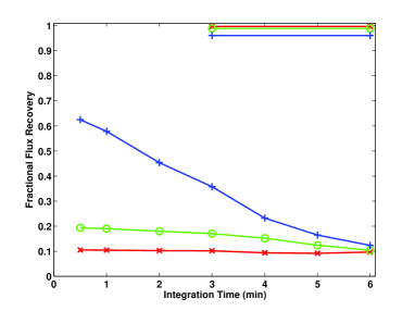
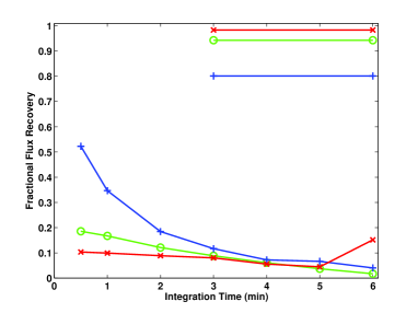
Figure 8: The fractional flux recovered versus integration time for the Frequency Phase Transfer (FPT) analysis of realistic simultaneous observations of pairs of frequencies, at 43/86 GHz (red; cross), 87/175 GHz (green; circle), and 175/350 GHz (blue; plus) under Very Good (Left), and Good (Right) weather conditions. The rms errors are smaller than the symbol size. Also shown in the top right are the values obtained using FPT plus a further self calibration iteration, following the same color and symbol codes.

4 Discussion

4.1 Comparative Performances

VLBI traditionally uses H-masers as frequency standards. Nevertheless, the short coherence times in observations at mm-VLBI can turn the H-maser instabilities into a significant limitation. We have carried out simulation studies to explore and compare the performance of H-masers and ultra stable CSOs in mm-VLBI observations, and quantify the impact with respect to that from the tropospheric fluctuations, under a variety of circumstances. Our simulations show that, in most situations, the tropospheric fluctuations constitute the dominant contribution to the coherence losses at mm and sub-mm wavelength observations; its impact increases with the observing frequency and/or worsening weather conditions, which in turn limits the coherence time and sensitivity. Hence, selecting sites with stable weather conditions is an essential step towards increasing the sensitivity of high frequency observations, as is well known. The impact of the coherence losses resulting from instabilities in the time standards in high frequency VLBI has been less explored. Its impact can be expected to be larger at higher frequencies. Our simulations show that at the highest frequencies, the losses induced by the H-maser instabilities are comparable to those from quality tropospheric conditions, for timescales comparable to the coherence times. For comparison, the corresponding losses for CSO instabilities are negligible ($<$0.5%). Hence, benefits from replacing the H-maser with a CSO for observations at the highest frequencies can be expected. In the other cases, the tropospheric fluctuations are the limiting contribution and there is little difference whether ones uses a H-maser or a CSO.
Figures 6 and 7 show the percent changes between the coherence losses for the H-maser and the CSO simulations as a function of integration time, in V and G weather conditions. For example, those are $\sim 2$, 7 and 14% at 86, 175 and 350 GHz, respectively, for $\sim 20\%$ coherence loss in the H-maser simulations with V weather conditions; and $\sim 1$, 3, 8% with G weather conditions. We conclude that the benefits, estimated by the reduction in coherence losses for the same integration time, of replacing the H-maser with a CSO are significant and $\geq 10\%$ for frequencies above 175 GHz (without WVR).

4.2 CSOs in VLBI Sites with Collocated WVRs

The use of co-located WVR in VLBI sites has the potential to greatly compensate the phase fluctuations induced by the tropospheric propagation into the astronomical signals. The measured effectiveness of the ALMA 183 GHz WVRs promises to provide a breakthrough for mm-VLBI observations (Honma, 2012; Matsushita et al., 2012) by enabling longer coherence times and hence higher sensitivity even at the highest frequencies and under a wider range of weather conditions. Its effect is roughly equivalent to an upgrade in the array weather conditions, which is dominated by the site with the poorest conditions, and will lead to the realization of a sub-mm VLBI array comprising multiple telescopes with ALMA-type weather conditions (i.e. upgraded from G to V).

The superior tropospheric compensation provided by co-located WVRs increases the significance of the H-maser instabilities and turn them into the dominant limitation in a much wider range of circumstances than shown in our simulations without WVR: i.e. over longer timescales, under more normal weather conditions, and for observations at lower frequencies. Maximum benefits are to be obtained from the combined operation of WVR and CSO at sub-mm VLBI sites.

Figure 9 shows the relative impact estimated for improved weather conditions as a result of using WVRs, for the more precise frequency standard, and for the combined effect of WVR and CSO in observations at 350 GHz. We estimate $\sim 10-20\%$ improved performance (i.e. reduced coherence loss) for observations under G weather conditions in a range of integration times from ten to a few tens of seconds, the typical coherence times found in VLBI observations at 1.3 mm with H-masers and no WVR corrections (Doeleman et al., 2011). Note that longer coherence times are expected as a result of the WVR atmospheric phase compensation and the ultra stable CSO, which result in an increase of the sensitivity. For comparison, at 175 GHz, a similar improvement is estimated for 0.5 to 1 minute timescales. Hence, we estimate significant benefits in combining WVRs and CSOs for VLBI observations at frequencies $\geq 175$ GHz.

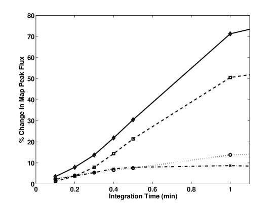
Figure 9: Comparative performances (i.e. percent change of coherence losses) of VLBI observations at 350 GHz versus integration times under different combinations of clocks and weather conditions: 1) impact of clock, using CSO instead of H-maser: CSO/G vs H-maser/G (dot-dash line) and CSO/V vs H-maser/V (dotted line); 2) impact of weather, using WVR to upgrade G to V conditions: H-maser/V vs H-maser/G (dash line); 3) combined effect of ultra stable clock and WVR: CSO/V vs. H-maser/G (solid line).

4.3 Increased Sensitivity Derived from Ultra Stable Frequency Standards.

In this section we take a different approach to compare the performances of H-maser and CSO in VLBI observations, in terms of sensitivity. Rather than comparing the coherence losses as a function of the integration time, here we compare the integration times that lead to identical losses, with the CSO and H-maser respectively, as a function of the coherence loss. The increase in sensitivity can be calculated as the square root of their ratio. Figure 10 shows the necessary CSO versus H-maser integration times for selected coherence losses between 2.5–40%, measured from simulations at 175 and 350 GHz under a variety of weather conditions. The locus of points for each of the frequency-weather combinations share similarities: the points are distributed, approximately, along lines parallel to y=x (the bottom-left to top-right diagonal); the total span is shorter for higher frequencies and worse weather conditions; the offset of each dataset from the diagonal increases with the quality of the weather conditions. For each point this offset is the difference between the integration times, for the CSO and H-maser cases, to reach an equal coherence loss. The sensitivity gain is the square root of the ratio of these integration times, as is indicated in the plot by the symbol size. Following this criterion, the increased sensitivity obtained from the CSO with respect to the H-maser in observations at 175 GHz with best (V) weather conditions are estimated to be 9% and 13%, for coherence losses of 20% and 10%, respectively; the equivalent values for good (G) weather conditions are 5% and 8%, respectively. At 350 GHz, the estimated increased sensitivity values are 22% and 41%, respectively, in V weather conditions. For G weather these are 11% and 18%. Maximum values of increased sensitivities are estimated for the case of WVR-corrected atmospheres (W) at 350 GHz, equal to 60% and 120%, for coherence losses of 20% and 10%, respectively. In all cases, the estimated values for increased sensitivities are larger for lower acceptable coherence losses. We conclude that there are significant sensitivity benefits, resulting from increased integration time, from replacing the H-maser with a ultra stable CSO, for observations at frequencies $\geq 175$ GHz, and that maximum benefits are obtained from using collocated WVRs to compensate for tropospheric fluctuations.

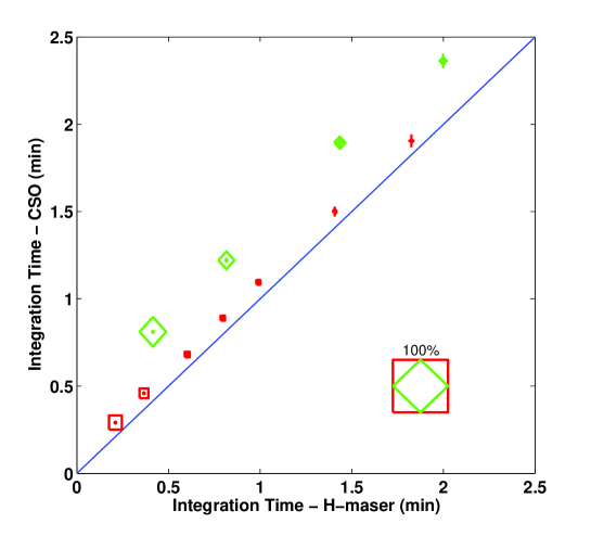
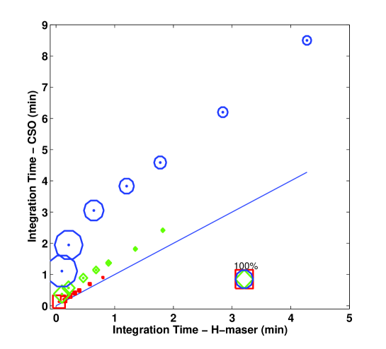
Figure 10: Comparison of integration times for matching coherence losses in complete simulations with CSO (y-axis) and H-maser (x-axis), under Very good (green diamond) and Good (red square)) weather conditions at 175 GHz (Upper), and additionally for WVR-corrected atmospheres (blue circle) at 350 GHz (Lower). Range of coherence losses displayed is: 2.5, 5, 10, 15, 20, 30, 40%; the points line up in the same order, with increasing distance from the origin. For each point, the size of the symbol corresponds to the log of the increased sensitivity value estimated from the use of the CSO compared to the H-maser for the corresponding coherence loss.

4.4 Application of CSOs in Space VLBI

Our simulations show the tendency for increasingly significant benefits to be gained from using CSOs (instead of H-masers) in VLBI observations at higher frequencies and under best weather conditions. Following these lines, space mm-VLBI, with no atmospheric propagation issues (at least for the space segment), provides the optimum case. Asaki & Miyoshi (2009) has proposed a low earth orbit satellite constellation, which provides excellent uv-coverage and highest angular resolution. This would observe at 350 GHz, focusing on studies of black hole environments. Based on our studies those advantages can be expected to be further increased, in terms of sensitivity, when combined with CSOs as time standards.

4.5 Dual-Frequency Observations and Analysis Strategies

Our simulations comprise the exploration of dual-frequency observations and phase transfer analysis to be used in mm-VLBI. Simultaneous dual-frequency observations are most desirable in the high frequency regime, in order to prevent the losses associated with switching. Our estimates show that even at 350 GHz, very small coherence losses (5% for V) can be obtained with integration times of many minutes, if the data are pre-calibrated using observations at 175 GHz. An alternative option to the self-calibration step is to include dual-frequency observations of a second source, with interleaving observations every few minutes; this is the basis of the Source Frequency Phase Referencing analysis (Rioja & Dodson, 2011), which provides spectral astrometry between the two frequency bands along with the increased coherence time for detection of weak sources. In both scenarios, the impact of tropospheric and clock instabilities, being of non-dispersive nature, are mitigated by the pre-calibration derived from the lower frequency. But fluctuations on timescales shorter than the pre-calibration integration times will remain. Here too benefits are to be gained by installation of WVR, to continuously correct for those errors arising from the troposphere. The benefits in terms of sensitivity are very significant, but should be considered along with the downside of the magnification of the noise, which sets limits on the minimum signal-to-noise ratio for observations of weak sources.

4.6 Extrapolation of Results to Higher Frequencies

We can extrapolate the results from our simulations at 86, 175 and 350 GHz to even higher frequencies using the trends shown in Figure 10. At frequencies $>350$ GHz, with best (V) weather conditions, the locus of points corresponding to the same range of coherence losses will spread along a line whose length will be shorter than that shown in the plot at 350 GHz, and the corresponding percentage increase in the sensitivities by use of CSOs with respect to H-masers will be larger. Using co-located WVRs, which will probably be mandatory at this frequency regime, will result in a vertical shift of this line in the plot, and in a net increase in the benefits of replacing the H-maser with a CSO. Hence, these results make a compelling case for use of CSOs in VLBI observations at the highest frequencies, beyond those in our simulations.

4.7 Possible Improvement of CSO Time Standards

The current CSO performance has potential for improvement. Both the 100 MHz and 10 MHz signals are synthesised from the microwave frequency of the oscillator which is determined by the natural resonance of the sapphire crystal (11.2-GHz). Due to the intrinsic phase noise of the hardware components that synthesize these frequencies, the 100 MHz is produced with much less degradation of the signal quality. Thus it is the recommended reference signal and is the frequency that has been used in these studies. Ongoing research also indicates that 1 GHz signals can be synthesized with even less degradation and such reference signals can now be transmitted over long distances with fiber techniques (e.g. Wilcox et al. (2009)). Thus the time standards no longer need to be on-site. Hence, should it be necessary in the future to further improve the CSO reference for the very highest observation frequencies there is still room for improvement. However we note that even in the best conditions, with WVR corrections, the atmospheric contributions are much greater than those from the CSO.

5 Conclusions

We have simulated realistic mm-VLBI data to address the importance of improving the frequency standards. We have extended the simulation tool ARIS to include H-maser and CSO instabilities, and allow for best quality and WVR-corrected atmospheric conditions. These simulated datasets reproduce well the expected behaviours from observational data. We have also explored the potential of dual-frequency observations to increase the coherence time at the higher frequencies in mm-VLBI observations. We conclude that, even at the highest frequencies, further calibration, such as Self-Calibration or SFPR, is required to produce useful results.

We have compared the coherence losses as a function of integration time using the simulations with H-maser and CSO, also we have estimated the improved sensitivity resulting from the increased integration time for a given allowable signal loss. We find that CSOs make a significant improvement at frequencies $\geq$175 GHz, under the best weather conditions. Using colocated WVRs to compensate for tropospheric fluctuations, we find the improvement to be even greater, and for a wider range of weather conditions.

References

- Asaki et al. (2010) Asaki, Y., Deguchi, S., Imai, H., et al. 2010, ApJ, 721, 267
- Asaki & Miyoshi (2009) Asaki, Y., & Miyoshi, M. 2009, in Astronomical Society of the Pacific Conference Series, Vol. 402, Approaching Micro-Arcsecond Resolution with VSOP-2: Astrophysics and Technologies, ed. Y. Hagiwara, E. Fomalont, M. Tsuboi, & M. Yasuhiro, 431
- Asaki et al. (2005) Asaki, Y., Saito, M., Kawabe, R., et al. 2005, Simulation Series of a Phase Calibration Scheme with Water Vapor Radiometers for the Atacama Compact Array, Tech. Rep. 535, ALMA,
- Asaki et al. (2007) Asaki, Y., Sudou, H., Kono, Y., et al. 2007, PASJ, 59, 397
- Beasley & Conway (1995) Beasley, A. J., & Conway, J. E. 1995, in Astronomical Society of the Pacific Conference Series, Vol. 82, Very Long Baseline Interferometry and the VLBA, ed. J. A. Zensus, P. J. Diamond, & P. J. Napier, 327
- Doeleman (2010) Doeleman, S. 2010, in 10th European VLBI Network Symposium and EVN Users Meeting: VLBI and the New Generation of Radio Arrays, 53
- Doeleman et al. (2011) Doeleman, S., Mai, T., Rogers, A. E. E., et al. 2011, PASP, 123, 582
- Greisen (2003) Greisen, E. W. 2003, Information Handling in Astronomy - Historical Vistas, 285, 109
- Hartnett & Nand (2010) Hartnett, J. G., & Nand, N. R. 2010, IEEE Transactions on Microwave Theory Techniques, 58, 3580
- Hartnett et al. (2012) Hartnett, J. G., Nand, N. R., & Lu, C. 2012, Applied Physics Letters, 100, 183501
- Hartnett et al. (2010) Hartnett, J. G., Nand, N. R., Wang, C., & Le Floch, J.-M. 2010, IEEE Trans on Ultrason. Ferro. Freq. Control, 57, 1034
- Honma (2012) Honma, M. 2012, Estimate of amplitude decorrelation based on band 6 data, Tech. Rep. CSV-1415, ALMA
- Matsushita et al. (2012) Matsushita, S., Morita, K., Barkats, D., et al. 2012, in Ground-based and Airborne Telescopes IV, 125 No. 8444 (Proceedings of SPIE)
- Middelberg et al. (2005) Middelberg, E., Roy, A. L., Walker, R. C., & Falcke, H. 2005, A&A, 433, 897
- Nand et al. (2011) Nand, N. R., Hartnett, J. G., Ivanov, E. N., & Santarelli, G. 2011, Microwave Theory and Techniques, 59, 2978
- Nikolic, et al. (2009) Nikolic, B., Richer, J., & Hills, R. 2009, USNC/URSI Annual Meeting
- Rioja & Dodson (2011) Rioja, M., & Dodson, R. 2011, AJ, 141, 114
- Rioja et al. (2011) Rioja, M., Dodson, R., Malarecki, J., & Asaki, Y. 2011, AJ, 142, 157
- Rogers et al. (1984) Rogers, A. E. E., Moffet, A. T., Backer, D. C., & Moran, J. M. 1984, Radio Science, 19, 1552
- Rogers & Moran (1981) Rogers, A. E. E., & Moran, Jr., J. M. 1981, IEEE Transactions on Instrumentation Measurement, 30, 283
- Thompson et al. (2007) Thompson, A. R., Moran, J. M., & Swenson, G. W. 2007, Interferometry and Synthesis in Radio Astronomy (John Wiley & Sons)
- Wang & Hartnett (2010) Wang, C., & Hartnett, J. 2010, Cryogenics
- Wilcox et al. (2009) Wilcox, R., Byrd, J. M., Doolittle, L., Huang, G., & Staples, J. W. 2009, Opt. Lett., 34, 3050