Time correlations and persistence probability of a Brownian particle in a shear flow.

Abstract

In this article, results have been presented for the two-time correlation functions for a free and a harmonically confined Brownian particle in a simple shear flow. For a free Brownian particle, the motion along the direction of shear exhibit two distinct dynamics, with the mean-square-displacement being diffusive at short times while at late times scales as $t^{3}$. In contrast the cross-correlation $\left\langle\left.x(t)y(t)\right.\right\rangle$ scales quadratically for all times. In the case of a harmonically trapped Brownian particle, the mean-square-displacement exhibits a plateau determined by the strength of the confinement and the shear. Further, the analysis is extended to a chain of Brownian particles interacting via a harmonic and a bending potential. Finally, the persistence probability is constructed from the two-time correlation functions.

1 Introduction

The phenomenon of persistence has been well studied over the past decade, both theoretically and experimentally Majumdar1999 ; Ray2004 . Persistence is the probability that a stochastic variable $x(t)$ retains a particular property up to the observation time interval $t$ – the property being either the sign of the variable or the crossing of the origin Ray2004 ; Majumdar1996 ; Bhattacharya2007 . The later definition of $p(t)$ is synonymous with the survival probability of the stochastic process, and the problem can also be approached using the backward Fokker-Planck equation. For a wide class of non-equilibrium systems, the asymptotic decay of $p(t)$ exhibits a power-law decay with a non-trivial exponent $\theta$. This algebraic decay, and the exponent, has been investigated for a wide class of non-interacting as well as interacting systems including the overdamped Brownian walker in an infinite Sire2000 ; Majumdar1999 and finite medium Chakraborty2007 , diffusion equation with random initial conditions Majumdar1996 ; Newman1998 , advection of a passive scalar Chakraborty2009 , fluctuating interfaces Krug1997 ; Toroczkai1999 ; Constantin2004 , critical dynamics Majumdar1996b , granular media Swift1999 ; Burkhardt2000 , disordered environments Fischer1998 ; Doussal1999 ; Chakraborty2008 and polymer dynamics Bhattacharya2007 . The probability $p(t)$ acts as a dynamic probe, indicating how the system retains the memory of its initial configuration as it evolves in time, and is also an indirect test for the two-time correlation functions for a non-stationary process. However, the estimation of the persistence probability is notoriously difficult and an exact analytical prediction for $p(t)$ at all times can be made only when the stochastic process is Gaussian and Markovian, such as, for an overdamped Brownian particle.

When the stochastic dynamics is a Gaussian Markovian process, the non-stationary process $x(t)$ can be mapped to a stationary Ornstein-Uhlenbeck process $\overline{X}(T)$, for which, the stationary correlator $C(T)\equiv\left\langle\left.\overline{X}(T)\overline{X}(0)\right.\right\rangle$ is exponentially decaying at all times. Asymptotically, the survival probability of the stationary Ornstein-Uhlenbeck process is proportional to $C(T)$ and $p(t)$ can be obtained by the inverse time transformation applied to $\overline{X}$ Majumdar1999 ; Slepian1962 . For a wide class of systems, the stationary correlator $C(T)$ is often non-exponential and this straight-forward method can no longer be applied. Using the classification of Slepian Slepian1962 , a correlator is of class $\alpha$, if $C(T)\sim 1-\mathcal{O}(T^{\alpha})$ in the limit of $T\to 0$. The behavior of $C(T)$ near zero characterizes the density of zero crossings $\rho$ of the stochastic process $\overline{X}$ Majumdar1996 ; Slepian1962 ; Rice1945 . When $\alpha=2$, the number of zero crossings is finite and the Independent Interval Approximation can be used to predict the exponent $\theta$ Majumdar1996 . If however, $\alpha<2$, the stochastic process has infinte number of zero crossings and a perturbative expansion gives a fairly good estimate for $\theta$ Krug1997 .

The case of a free Brownian particle, in the overdamped limit, is particularly simple and illustrates how the persistence probability can be determined for a Gaussian Markov process Slepian1962 . We define the persistence probability as the probability that the particle has not crossed the origin during the observation time interval $t$. Even though the system under consideration is very simple, its application is abundant in quantitative science Frey2005a . The two-time correlation function for the non-stationary process $x(t)=\int_{0}^{t}\eta(t^{\prime})\mathrm{d}t^{\prime}$, where $\eta$ is a Gaussian stochastic noise, can be transformed into a stationary Ornstein-Uhlenbeck process using the successive transformations $\overline{X}\equiv x/\sqrt{\left\langle\left.x^{2}(t)\right.\right\rangle}$ and $T=\ln t$. The stationary correlator of $\overline{X}$ is then given by $e^{-T/2}$, and following Ref.Slepian1962 , the persistence probability in the transformed variable decays exponentially – $P(T)\sim e^{-T/2}$. Using the reverse transformation, the decay of $p(t)$ in real time becomes algebraic with an exponent $\theta=1/2$.

In this article, we investigate the persistence probability of a free and confined Brownian particle in a shear flow and that of an interacting chain of Brownian particles. The work is motivated on one hand by the extensive theoretical SanMiguel1979 ; Taylor1953 ; Yoshishige1996 ; Kienle2011 ; Bammert2010 and experimental Orihara2011 study of Brownian motion in a linear shear flow and their importance in microfluidic applications, and on the other hand, due to the rich dynamics exhibited by such systems as a result of an interplay of thermal fluctuations and the imposed velocity gradient Perkins1997 ; Groisman2001 ; Groisman2000 . The investigation of the survival probability for a free Brownian particle in a deterministic flow field $v(x)$ has been previously investigated Bray2006 ; Bray2005 ; Bray2004 , and is known that for all odd functions of $v(x)$ the survival probability decays as $t^{-1/4}$. However, all of these approaches use the Fokker-Planck equation to determine the survival probability. In the present work, we emphasize on the two-time correlation function and present explicit results for them for the case of a free and harmonically confined Brownian particle in a transverse flow field. In the case of a chain of Brownian particles harmonically bounded to its nearest neighbors, we impose an additional bending potential to mimic the case of a semi-flexible polymer chain.

The rest of the article is organized as follows: the model system is introduced in sec:simple_shear. The relevant results for the two-time correlation functions and the persistence probability for a free Brownian particle is presented in sec:simple_shear, and for a confined Brownian particle, in sec:harmonically_bound. We extend the analysis presented in the previous sections to a chain of interacting Brownian particles and present the results in sec:interacting_chain.

2 Brownian particle in a shear flow

The stochastic dynamics of a Brownian particle can be looked at from different levels of coarse-graining. Typically, if the measurement time intervals of the position and momenta of a colloid are well separated, the Markovian Langevin equation in the overdamped limit faithfully reproduces the dynamics. In reality, however, the dynamics of a Brownian particle exhibit a far more rich physics. As opposed to the Markovian Langevin equation, characterized by a single relaxation time, the actual dynamics of Brownian particle is characterized by a set of time-scales determined by sound propagation, vorticity diffusion and the inertia of the colloid. As a consequence, the motion of the Brownian particle no longer remains Markovian and the generalized Markovian equation with a memory dependent friction and a correlated noise is used to describe the dynamics. With this increasing level of complexity, an analytically tractable result becomes difficult and one has to resort to a numerical integration of the equations of motion. In the following, however, we consider the overdamped Langevin equation to describe the dynamics, neglecting the effects of solvent and the inertia of the Brownian particle.

We consider the motion of a Brownian particle, with a unit mass, in an unbounded solvent moving in a two-dimensional planar geometry. Following SanMiguel1979 , we consider a stationary distribution of velocity,

$$\mathbf{u}=(0,ax).$$ (1)

The force on the Brownian particle, due to the imposed flow is given by $\mathbf{F}=-\zeta(\mathbf{v}-\mathbf{u})$, where $\mathbf{v}$ is the instantaneous velocity of the particle and $\zeta$ is the Stokes’s friction on the colloid. The Langevin equation for the position of a colloid $\mathbf{r}\equiv(x,y)$, in the overdamped limit, takes the form

$$\frac{\mathrm{d}x}{\mathrm{d}t}=\eta_{x}(t)\quad\quad\quad\textrm{and}\quad\quad\quad\frac{\mathrm{d}y}{\mathrm{d}t}=ax+\eta_{y}(t),$$ (2)

with $\boldsymbol{\eta}\equiv(\eta_{x},\eta_{y})$ as a Gaussian white noise with correlations

$$\left\langle\left.\boldsymbol{\eta}(t)\right.\right\rangle=0\quad\quad\quad\textrm{and}\quad\quad\quad\left\langle\left.\boldsymbol{\eta}(t)\otimes\boldsymbol{\eta}(t^{\prime})\right.\right\rangle=2D\mathbf{I}\delta(t-t^{\prime}),$$ (3)

where $\mathbf{I}$ is the identity matrix and $\otimes$ denote the outer product of a vector quantity. The strength of the noise correlations is given by the diffusion constant $D=k_{\rm B}T/\zeta$. The two-time correlation functions from eq:langevin becomes,

$$\left\langle\left.x(t_{1})x(t_{2})\right.\right\rangle=\int_{0}^{t_{1}}\mathrm{d}t_{1}^{\prime}\int_{0}^{t_{2}}\mathrm{d}t_{2}^{\prime}\left\langle\left.\eta_{x}(t_{1}^{\prime})\eta_{x}(t_{2}^{\prime})\right.\right\rangle$$ (4)

and

$$\left\langle\left.y(t_{1})y(t_{2})\right.\right\rangle=\int_{0}^{t_{1}}\mathrm{d}t_{1}^{\prime}\int_{0}^{t_{2}}\mathrm{d}t_{2}^{\prime}\;\left\langle\left.\eta_{y}(t_{1}^{\prime})\eta_{y}(t_{2}^{\prime})\right.\right\rangle\\ +a^{2}\int_{0}^{t_{1}}\mathrm{d}t_{1}^{\prime}\int_{0}^{t_{2}}\mathrm{d}t_{2}^{\prime}\;\left\langle\left.x(t_{1}^{\prime})x(t_{2}^{\prime})\right.\right\rangle.$$ (5)

Assuming $t_{1}>t_{2}$, eq:twotimex yields $\left\langle\left.x(t_{1})x(t_{2})\right.\right\rangle=2Dt_{2}$ and

$$\left\langle\left.y(t_{1})y(t_{2})\right.\right\rangle=2Dt_{2}+a^{2}\int_{0}^{t_{1}}\mathrm{d}t_{1}^{\prime}\int_{0}^{t_{2}}\mathrm{d}t_{2}^{\prime}\min(t_{1}^{\prime},t_{2}^{\prime}).$$ (6)

The integral on the right-hand-side of eq:twotimey1 evaluates to

$$\left\langle\left.y(t_{1})y(t_{2})\right.\right\rangle=2Dt_{2}+a^{2}D\left(t_{1}t_{2}^{2}-\frac{t_{2}^{3}}{3}\right).$$ (7)

Similarly, the cross-correlation functions $\left\langle\left.x(t_{1})y(t_{2})\right.\right\rangle$ and $\left\langle\left.y(t_{1})x(t_{2})\right.\right\rangle$ can be constructed as,

$$\left\langle\left.x(t_{1})y(t_{2})\right.\right\rangle=a\int_{0}^{t_{1}}\mathrm{d}t_{1}^{\prime}\int_{0}^{t_{2}}\mathrm{d}t^{\prime}_{2}\;\,\left\langle\left.\eta_{x}(t^{\prime}_{1})x(t_{2}^{\prime})\right.\right\rangle\\ +\int_{0}^{t_{1}}\mathrm{d}t_{1}^{\prime}\int_{0}^{t_{2}}\mathrm{d}t^{\prime}_{2}\;\,\left\langle\left.\eta_{x}(t^{\prime}_{1})\eta_{y}(t_{2}^{\prime})\right.\right\rangle,$$ (8)

and

$$\left\langle\left.y(t_{1})x(t_{2})\right.\right\rangle=a\int_{0}^{t_{1}}\mathrm{d}t_{1}^{\prime}\int_{0}^{t_{2}}\mathrm{d}t^{\prime}_{2}\;\,\left\langle\left.x(t^{\prime}_{1})\eta_{x}(t^{\prime}_{2})\right.\right\rangle\\ +\int_{0}^{t_{1}}\mathrm{d}t_{1}^{\prime}\int_{0}^{t_{2}}\mathrm{d}t^{\prime}_{2}\;\,\left\langle\left.\eta_{x}(t^{\prime}_{1})\eta_{y}(t_{2}^{\prime})\right.\right\rangle.$$ (9)

The second terms in both of the above equation are zero due to the choice of the noise correlations in eq:noisecorr. Further, using the solution $x(t)=\int_{0}^{t}\mathrm{d}t^{\prime}\eta_{x}(t^{\prime})$, the correlation function in eq:cross_corr_xy becomes,

$$\left\langle\left.x(t_{1})y(t_{2})\right.\right\rangle=a\int_{0}^{t_{2}}\mathrm{d}t^{\prime}_{2}\int_{0}^{t_{1}}\mathrm{d}t_{1}^{\prime}\int_{0}^{t^{\prime}_{2}}\mathrm{d}t^{\prime\prime}_{2}\;\,\left\langle\left.\eta_{x}(t^{\prime}_{1})\eta(t^{\prime\prime}_{2})\right.\right\rangle=Dat_{2}^{2},$$ (10)

and the correlation function in eq:cross_corr_yx evaluates to,

$$\begin{split}\left\langle\left.y(t_{1})x(t_{2})\right.\right\rangle&=a\int_{0}^{t_{1}}\mathrm{d}t_{1}^{\prime}\int_{0}^{t_{2}}\mathrm{d}t^{\prime}_{2}\int_{0}^{t^{\prime}_{1}}\mathrm{d}t^{\prime\prime}_{1}\;\,\left\langle\left.\eta_{x}(t^{\prime\prime}_{1})\eta_{x}(t^{\prime}_{2})\right.\right\rangle\\ &=2Da\int_{0}^{t_{1}}\mathrm{d}t^{\prime}_{1}\min(t_{2},t^{\prime}_{1})=2Da\left(t_{1}t_{2}-\frac{t_{2}^{2}}{2}\right).\end{split}$$ (11)

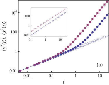
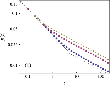
Figure 1: (a) Mean-square displacement of a Brownian particle in a simple shear along the $y$ direction for $a=1.00$ ( $\bullet$) and $5.00$ ( $\blacksquare$). The corresponding mean-square displacement along the $x$-direction is shown for $a=1.00$ ( $\circ$) only. The solid lines are the plots of eq:msdy for the respective values of $a$ and the dot-dashed line is the plot of $\left\langle\left.x^{2}(t)\right.\right\rangle=2Dt$. Inset: Plot of $\left\langle\left.x(t)y(t)\right.\right\rangle$ for $a=1.00$ ( $\vartriangle$) and $5.00$ ( $\triangledown$). The dashed line are the plots of eq:xyt. (b) Persistence probability of a Brownian particle in a simple shear for ( $\bullet$), $5.00$ ( $\blacksquare$) and $10.0$ ( $\blacktriangle$). The dashed line is plot of $t^{-1/2}$ corresponding to that of a free Brownian particle, while the dot dashed line is a plot of $t^{-1/4}$.

Using the two-time correlation functions evaluated above, we can construct the corresponding mean-square displacements by simply substituting $t_{2}=t_{1}=t$. Along the $x$-direction the motion remains purely diffusive, while the mean-square-displacement of the particle along the $y$-direction becomes,

$$\left\langle\left.y^{2}(t)\right.\right\rangle=2Dt+\frac{2}{3}a^{2}Dt^{3}.$$ (12)

For short times, $t<<a^{-1}$, the motion of the Brownian particle along the $y$-direction is purely diffusive, while in the asymptotic regime of $t>>a^{-1}$ the mean-square-displacement scales as $t^{3}$ – similar to that of a randomly accelerated particle.

The cross-correlation function $\left\langle\left.x(t)y(t)\right.\right\rangle$, however, has two contributions and adding up eq:corr_xy_1 and eq:corr_yx_1 gives,

$$\left\langle\left.x(t)y(t)\right.\right\rangle=Dat^{2}.$$ (13)

Our aim is to extract the persistence probability of the Brownian particle using the correlation function defined in eq:twotimey2. To this end, we define it as the probability that the $y$-component of the particle position has not crossed zero. The fundamental idea is to map the non-stationary process $y(t)$ to a stationary Ornstein-Uhlenbeck (O-U) process $\overline{Y}$. The stationary correlator $C(T)$ for $\overline{Y}$ decays exponentially for all times and the persistence probability can be shown to decay as $P(T)\sim\frac{2}{\pi}\sin^{-1}[C(T)]$ Slepian1962 ; Majumdar2001 . The mapping to the stationary O-U process is done using two transformations, first normalizing the stochastic variable by the root-mean-square displacement and then a suitable transformation in time. For the correlation function in eq:twotimey2, the transformation $\overline{Y}=y(t)/\sqrt{\left\langle\left.y^{2}(t)\right.\right\rangle}$ yields,

$$\left\langle\left.\overline{Y}(t_{1})\overline{Y}(t_{2})\right.\right\rangle=\dfrac{2Dt_{2}+a^{2}D\left(t_{1}t_{2}^{2}-\dfrac{t_{2}^{3}}{3}\right)}{\left(2Dt_{1}+\frac{2}{3}a^{2}Dt_{1}^{3}\right)^{1/2}\left(2Dt_{1}+\frac{2}{3}a^{2}Dt_{1}^{3}\right)^{1/2}}$$ (14)

A suitable time transformation which converts eq:Y1Y2 to a stationary process for all times is non-trivial. However, we can extract persistence probability by considering the limiting behaviors of eq:Y1Y2. As noted above, for $t\ll a^{-1}$, the motion of the colloid is purely diffusive and neglecting the $\mathcal{O}(t^{3})$ terms gives,

$$\left\langle\left.\overline{Y}(t_{1})\overline{Y}(t_{2})\right.\right\rangle=\sqrt{\dfrac{t_{2}}{t_{1}}}.$$ (15)

In the opposite limit of $t\gg a^{-1}$, the linear term can be neglected and the correlation function for the normalized variable becomes,

$$\left\langle\left.\overline{Y}(t_{1})\overline{Y}(t_{2})\right.\right\rangle=\frac{3}{2}\left(\frac{t_{2}}{t_{1}}\right)^{1/2}-\frac{1}{2}\left(\frac{t_{2}}{t_{1}}\right)^{3/2}$$ (16)

Using the time transformation $e^{T}=t$, eq:Y1Y2_short and eq:Y1Y2_long are transformed to a Gaussian stationary process with correlations,

$$C(T)=\begin{cases}e^{-T/2}&\mbox{for }t\ll a^{-1}\\ \frac{3}{2}e^{-T/2}-\frac{1}{2}e^{-3T/2}&\mbox{for }t\gg a^{-1}.\end{cases}$$ (17)

Since the stationary correlator for $t<a^{-1}$ is exponentially decaying, the persistence probability in the transformed variable $T$ is given by $P(T)\sim e^{-T/2}$ and in real time $p(t)\sim t^{-1/2}$. In the asymptotic regime, the correlation function corresponds to that of a randomly accelerated particle and the persistence probability is known from the works of Sinai and Burkhardt Sinai1992 ; Burkhardt2000 to decay as $p(t)\sim t^{-1/4}$.

To validate the results presented above, numerical simulations were done by integrating eq:langevin using the Euler scheme with an integration time step of $\mathrm{d}t=0.001$. From this numerical integration, the position of the particle in the subsequent time steps were measured and the mean-square-displacement along and perpendicular to the direction of the applied shear, as well as the cross-correlation functions were computed. The results of the numerical simulation is presented in the left panel of fig:msdplot_freebm and compared to the analytical results of eq:msdy and eq:xyt. The measured data were averaged over $10^{5}$ independent configurations. In all of these simulation runs, the particle was started in the neighborhood of zero, so that the sign of $y(0)$ is defined and subsequently the sign of $y(t)$ was followed. The fraction of particles for which the sign of $y(t)$ did not change quantified the persistence probability. The measured persistence probability for the Brownian particle in the direction of the applied shear is shown in the right panel of fig:msdplot_freebm. The measured probability exhibits two distinct regimes of decay, for $t<<a^{-1}$ a decay of $t^{-1/2}$ and for $t>>a^{-1}$ a decay of $t^{-1/4}$.

3 Harmonically confined Brownian particle in a shear flow

In this section we study the dynamics of a tracer in a simple shear flow which is also confined by a harmonic potential. The harmonic confinement occurs naturally in the experiments when a tracking of a tracer is done using an optical tweezers. The equations of motion for the position of a colloid which is subjected to a harmonic confinement $U(r)=\frac{1}{2}\kappa r^{2}$ and the stationary velocity profile of eq:velprf are,

$$\frac{\mathrm{d}x}{\mathrm{d}t}=-\kappa x+\eta_{x}(t)\;\;\;\textrm{and}\;\;\;\frac{\mathrm{d}y}{\mathrm{d}t}=-\kappa y+ax+\eta_{y}(t),$$ (18)

together with the noise correlations of eq:noisecorr. The time evolution of the coordinates is given by,

$$\begin{split}x(t)=\int_{0}^{t}\mathrm{d}t^{\prime}e^{-\kappa(t-t^{\prime})}\eta_{x}(t^{\prime})\;\;\mbox{and}\;\;\\ y(t)=\int_{0}^{t}\mathrm{d}t^{\prime}e^{-\kappa(t-t^{\prime})}\left[x(t^{\prime})+\eta_{y}(t^{\prime})\right].\end{split}$$ (19)

Assuming that $t_{1}>t_{2}$, the two-time correlation function for the variable $x(t)$ is straightforward and gives,

$$\left\langle\left.x(t_{1})x(t_{2})\right.\right\rangle=\frac{D}{\kappa}\left[e^{-\kappa(t_{1}-t_{2})}-e^{-\kappa(t_{1}+t_{2})}\right]$$ (20)

while for $y(t)$ we have,

$$\begin{split}\left\langle\left.y(t_{1})y(t_{2})\right.\right\rangle=\frac{a^{2}D}{\kappa}e^{-\kappa(t_{1}+t_{2})}\int_{0}^{t_{1}}\mathrm{d}t^{\prime}_{1}\int_{0}^{t_{2}}\mathrm{d}t^{\prime}_{2}\;\,e^{\kappa(t^{\prime}_{1}+t^{\prime}_{2})}\left[e^{-\kappa|t^{\prime}_{1}-t^{\prime}_{2}|}-\right.\\ \left.e^{-\kappa(t^{\prime}_{1}+t^{\prime}_{2})}\right]+\int_{0}^{t_{1}}\mathrm{d}t^{\prime}_{1}\int_{0}^{t_{2}}\mathrm{d}t^{\prime}_{2}\;\,\left\langle\left.\eta_{y}(t^{\prime}_{1})\eta_{y}(t^{\prime}_{2})\right.\right\rangle.\end{split}$$ (21)

The integral over $t^{\prime}_{1}$ and $t^{\prime}_{2}$ yields,

$$\left\langle\left.y(t_{1})y(t_{2})\right.\right\rangle=\frac{a^{2}D}{2\kappa^{3}}\left[\left(e^{-\kappa(t_{1}-t_{2})}-e^{-\kappa(t_{1}+t_{2})}\right)\right.\\ -\kappa\left((t_{1}+t_{2})e^{-\kappa(t_{1}+t_{2})}-(t_{1}-t_{2})e^{-\kappa(t_{1}-t_{2})}\right)\\ -\left.2\kappa^{2}\;t_{1}t_{2}e^{-\kappa(t_{1}+t_{2})}\right]+\frac{D}{\kappa}\left[e^{-\kappa(t_{1}-t_{2})}-e^{-\kappa(t_{1}+t_{2})}\right]$$ (22)

The mean-square displacement for $y(t)$ immediately follows from eq:two_time_hc_y1 via a substitution $t_{1}=t_{2}=t$,

$$\left\langle\left.y^{2}(t)\right.\right\rangle=\frac{a^{2}D}{2\kappa^{3}}\left[\left(1-e^{-2\kappa t}\right)+2\kappa te^{-2\kappa t}-2\kappa^{2}t^{2}e^{-2\kappa t}\right]\\ +\frac{D}{\kappa}\left[1-e^{-2\kappa t}\right].$$ (23)

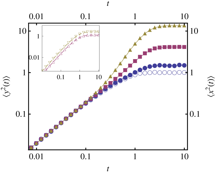
Figure 2: Mean-square displacement of a Brownian particle in a simple shear along the $y$ direction for $a=1.00$ ( $\bullet$), $2.50$ ( $\blacksquare$) and $5.00$ ( $\blacktriangle$). The corresponding mean-square displacement along the $x$-direction is shown for $a=1.00$ ( $\circ$) only. The solid lines are the plots of eq:msd_hc_y for the respective values of $a$ and the dot-dashed line is the plot of $\left\langle\left.x^{2}(t)\right.\right\rangle=2Dt$. Inset: Plot of $\left\langle\left.x(t)y(t)\right.\right\rangle$ for $a=2.50$ ( $\vartriangle$) and $5.00$ ( $\triangledown$). The dashed line are the plots of eq:hc_xy_t.

Further, the cross-correlation functions $\left\langle\left.x(t_{1})y(t_{2})\right.\right\rangle$ and
$\left\langle\left.y(t_{1})x(t_{2})\right.\right\rangle$ is given by,

$$\left\langle\left.x(t_{1})y(t_{2})\right.\right\rangle=\int_{0}^{t_{2}}\mathrm{d}t^{\prime}_{2}\;\;e^{-\kappa(t_{2}-t^{\prime}_{2})}\left\langle\left.x(t_{1})x(t^{\prime}_{2})\right.\right\rangle\\ =\frac{aD}{2\kappa^{2}}\left[e^{-\kappa(t_{1}-t_{2})}-e^{-\kappa(t_{1}+t_{2})}-2\kappa t_{2}e^{-\kappa(t_{1}+t_{2})}\right]$$ (24)

$$\left\langle\left.y(t_{1})x(t_{2})\right.\right\rangle=\int_{0}^{t_{1}}\mathrm{d}t^{\prime}_{1}\;\;e^{-\kappa(t_{1}-t^{\prime}_{1})}\left\langle\left.x(t^{\prime}_{1})x(t_{2})\right.\right\rangle\\ =\frac{aD}{\kappa}\int_{0}^{t_{1}}\mathrm{d}t^{\prime}_{1}\;\;e^{-\kappa(t_{1}-t^{\prime}_{1})}\left[e^{-\kappa|t^{\prime}_{1}-t_{2}|}-e^{-\kappa(t^{\prime}_{1}+t_{2})}\right]$$ (25)

The integral over $t^{\prime}_{1}$ in eq:corr_hc_yx gives,

$$\left\langle\left.y(t_{1})x(t_{2})\right.\right\rangle=\frac{aD}{2\kappa^{2}}\left[e^{-\kappa(t_{1}-t_{2})}-e^{-\kappa(t_{1}+t_{2})}+2\kappa(t_{1}-t_{2})e^{-\kappa(t_{1}-t_{2})}\right.\\ \left.-2\kappa t_{1}e^{-\kappa(t_{1}+t_{2})}\right]$$ (26)

The cross-correlation function $\left\langle\left.x(t)y(t)\right.\right\rangle$ is obtained by adding eq:corr_hc_xy and eq:corr_hc_yx1 and the substitution $t_{1}=t_{2}=t$ which gives,

$$\left\langle\left.x(t)y(t)\right.\right\rangle=\frac{aD}{2\kappa^{2}}\left[1-e^{-2\kappa t}-2\kappa te^{-2\kappa t}\right]$$ (27)

A Taylor expansion of eq:msd_hc_y for $t<\kappa^{-1}$, shows that the dynamics at short times scales as $2Dt+(2/3)a^{2}Dt^{3}$, while in the asymptotic regime, the mean-square displacement saturates to a value $D/\kappa+a^{2}D/\kappa^{3}$. To determine the persistence probability, we follow the steps outlined in the previous section. However, an expression for the persistence probability valid at all times is once again not feasible. Even in the asymptotic regime, a suitable time transformation does not exist which converts the process $y(t)$ to a Gaussian stationary process. Progress can only be made in the time domain which is smaller than $\kappa^{-1}$, where the two-time correlation function is identical to eq:twotimey2. Accordingly, the persistence probability shows an initial decay of $t^{-1/2}$, followed by a decay of $t^{-1/4}$. The mean-square-displacement of the harmonically confined Brownian particle in a simple shear flow is shown in fig:msd_hc. Once again, the integration of eq:langevin_harmonic was carried out using the Euler scheme with an integration time step of $\mathrm{d}t=0.001$. The measured mean-square-displacement is compared to the analytical prediction of eq:msd_hc_y in the main figure, while the inset depicts the cross-correlation function $\left\langle\left.x(t)y(t)\right.\right\rangle$ for two different values of $a$, defined in eq:velprf.

4 Interacting chain of Brownian particles

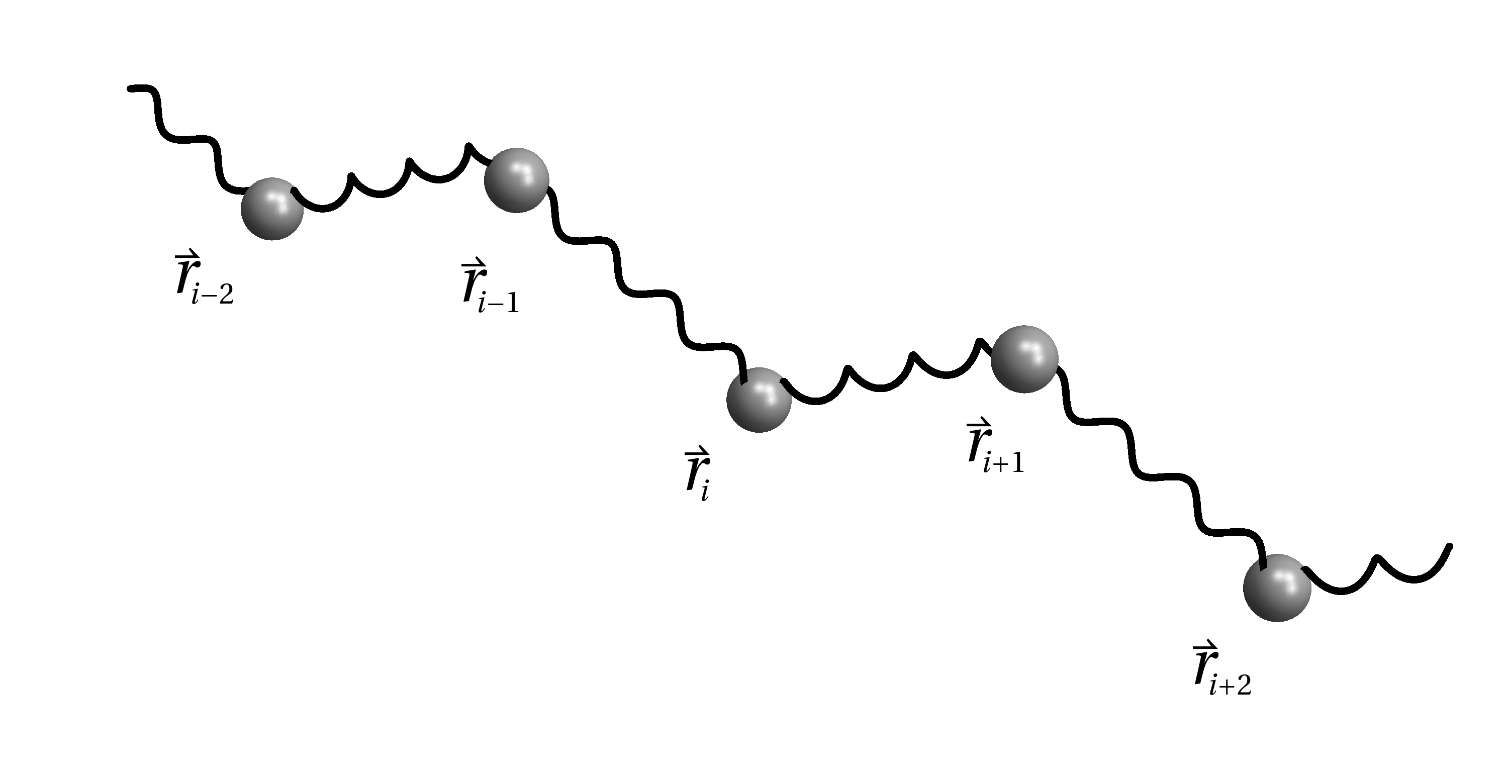
Figure 3: Artistic illustration of a bead-spring model of a polymer. In addition to the harmonic confinement between the beads, an angular confinement is also implemented.

In this section, we investigate the persistence probability of an interacting chain of $N$ Brownian particles, in a two-dimensional planar solvent subjected to the stationary flow of eq:velprf. In addition to the harmonic confinement $U(r)=\frac{1}{2}\kappa(r-R_{0})^{2}$ of a particle to its nearest neighbors, we impose a bending potential

$$U^{\;\textrm{bend}}(\theta)=\sum_{j=2}^{N-1}\frac{\kappa_{\theta}}{2}(1+\mathbf{\hat{u}}_{j}\mathbf{\hat{u}}_{j-1})^{2},$$ (28)

where $\mathbf{\hat{u}}_{i}=\mathbf{r}_{i+1}-\mathbf{r}_{i}/|\mathbf{r}_{i+1}-\mathbf{r}_{i}|$. This discrete model of a chain of Brownian particle is often used in simulations to model semi-flexible polymer chains Pham2008 ; Manghi2006 . In the absence of the bending potential, the model corresponds to that of a Rouse chain and the persistence probability of such a chain in a simple shear flow has been studied by Bhattacharya et al.Bhattacharya2007 . The resulting expression for the bending force takes the form,

$$\mathbf{f}^{\;\textrm{bend}}_{i}=-\kappa_{\theta}\sum_{j=2}^{N-1}(1+\mathbf{\hat{u}}_{j}\mathbf{\hat{u}}_{j-1})\dfrac{\partial}{\partial\mathbf{r}_{i}}\mathbf{\hat{u}}_{j}\mathbf{\hat{u}}_{j-1}$$ (29)

Using the explicit form of $\mathbf{\hat{u}}_{i}$, and assuming that the confinement strength of the harmonic force and the bending rigidity is sufficiently large so that we are in weakly bending limit, such that $|\mathbf{\hat{u}}(i+1)-\mathbf{\hat{u}}(i)|\ll 1$ Morse1998 , the force on particle $i$ becomes,

$$\mathbf{f}^{\;\textrm{bend}}_{i}=-2\frac{\kappa_{\theta}}{R_{0}^{4}}(-\mathbf{r}_{i-2}+4\mathbf{r}_{i-1}-6\mathbf{r}_{i}+4\mathbf{r}_{i+1}-\mathbf{r}_{i+2}),$$ (30)

with $R_{0}$ as the inter-particle separation. Note that in this approximation, the force due to the harmonic confinement can be neglected. The equation of a Brownian particle then becomes,

$$\begin{split}\frac{\mathrm{d}x_{i}}{\mathrm{d}t}&=-2\frac{\kappa_{\theta}}{R_{0}^{4}}(-x_{i-2}+4x_{i-1}-6x_{i}+4x_{i+1}-x_{i+2})+\eta_{x}(i,t)\\ \frac{\mathrm{d}y_{i}}{\mathrm{d}t}&=-2\frac{\kappa_{\theta}}{R_{0}^{4}}(-y_{i-2}+4y_{i-1}-6y_{i}+4y_{i+1}-y_{i+2})+ax_{i}(t)+\eta_{y}(i,t)\end{split}$$ (31)

The above equations are only valid for $N-4$ particles, and the $4$ particles at the boundary will have different equations of motion. However, for an infinitely long chain, the monomer dynamics at late times is not sensitive to the boundary conditions and accordingly a continuum version of the equations can be formulated by replacing $i$ with a continuous variable $s$,

$$\begin{split}\frac{\partial}{\partial t}\!\!\!\genfrac{}{}{0.0pt}{}{x(s,t)}{}&=-\overline{\kappa}\;\frac{\partial^{4}}{\partial s^{4}}\!\!\!\genfrac{}{}{0.0pt}{}{x(s,t)}{}+\eta_{x}(s,t)\\ \\ \frac{\partial}{\partial t}\!\!\!\genfrac{}{}{0.0pt}{}{y(s,t)}{}&=-\overline{\kappa}\;\frac{\partial^{4}}{\partial s^{4}}\!\!\!\genfrac{}{}{0.0pt}{}{y(s,t)}{}+ax(t)+\eta_{y}(s,t)\end{split}$$ (32)

Fourier transforming the above equations leads to,

$$\frac{\partial\tilde{x}}{\partial t}=-\overline{\kappa}\;k^{4}\;\tilde{x}(k,t)+\tilde{\eta}_{x}(k,t)\\$$ (33)

$$\frac{\partial\tilde{y}}{\partial t}=-\overline{\kappa}\;k^{4}\;\tilde{y}(k,t)+a\tilde{x}(k,t)$$ (34)

We have dropped the stochastic noise term in eq:langevin_ft_y, since at late-times the second term $ax(t)$ becomes the dominant term compared to the stochastic force. The formal solutions of eq:langevin_ft_x and eq:langevin_ft_y are given by,

$$\tilde{x}(k,t)=\int_{0}^{t}\;\mathrm{d}t^{\prime}\;e^{-\overline{\kappa}\;k^{4}\;(t-t^{\prime})}\;\tilde{\eta}_{x}(k,t^{\prime})$$ (35)

$$\tilde{y}(k,t)=\int_{0}^{t}\;\mathrm{d}t^{\prime}\;e^{-\overline{\kappa}\;k^{4}\;(t-t^{\prime})}\;\tilde{x}(k,t^{\prime}).$$ (36)

Using the noise correlation for $\left\langle\left.\tilde{\eta}_{x}(k,t)\tilde{\eta}_{x}(k^{\prime},t)\right.\right\rangle=2D\delta(k+k^{\prime})\delta(t-t^{\prime})$, the two-time correlation function for $\tilde{x}$ reads,

$$\left\langle\left.\tilde{x}(k,t_{1})\tilde{x}(k^{\prime},t_{2})\right.\right\rangle =\frac{D}{\overline{D}(k)}\delta(k+k^{\prime})e^{-\overline{D}(k)(t_{1}+t_{2})}\left[e^{2\overline{D}(k)\min(t_{1},t_{2})}-1\right]$$

$$=\frac{D}{\overline{D}(k)}\delta(k+k^{\prime})\left[e^{-\overline{D}(k)(t_{1}-t_{2})}-e^{-\overline{D}(k)(t_{1}+t_{2})}\right],$$ (37)

where $\overline{D}(k)=\overline{\kappa}k^{4}$ is the diffusion coefficient of a mode $k$. The second line of eq:two_time_x assumes $t_{1}>t_{2}$. Similarly, the two-time correlation function for the $y(s,t)$ can be constructed from eq:two_time_x,

$$\left\langle\left.y(s,t_{1})y(s,t_{2})\right.\right\rangle=a^{2}\int\frac{\mathrm{d}k_{1}}{2\pi}\int\frac{\mathrm{d}k_{2}}{2\pi}e^{-(k_{1}+k_{2})s}\int_{0}^{t_{1}}\mathrm{d}t^{\prime}_{1}\int_{0}^{t_{2}}\mathrm{d}t^{\prime}_{2}\\ e^{-\overline{D}(k_{1})(t_{1}-t^{\prime}_{1})}e^{-\overline{D}(k_{2})(t_{2}-t^{\prime}_{2})}\left\langle\left.\tilde{y}(k_{1},t^{\prime}_{1})\tilde{y}(k_{2},t^{\prime}_{2})\right.\right\rangle$$ (38)

Substituting eq:two_time_x in the equation above and subsequently integrating over the delta function and renaming the dummy variable $k_{1}$ we arrive at,

$$\left\langle\left.y(s,t_{1})y(s,t_{2})\right.\right\rangle=a^{2}\int\frac{\mathrm{d}k}{2\pi}\int_{0}^{t_{1}}\mathrm{d}t^{\prime}_{1}\int_{0}^{t_{2}}\mathrm{d}t^{\prime}_{2}\;e^{-\overline{D}(k)(t_{1}+t_{2})}\;\\ \frac{D}{\overline{D}(k)}\;\left[e^{2\overline{D}(k)\min(t^{\prime}_{1},t^{\prime}_{2})}-1\right]\\ =\frac{a^{2}D}{\overline{\kappa}}\int_{0}^{t_{1}}\mathrm{d}t^{\prime}_{1}\int_{0}^{t_{2}}\mathrm{d}t^{\prime}_{2}\left[\int\frac{\mathrm{d}k}{2\pi}\frac{1-e^{-\overline{\kappa}k^{4}(t_{1}+t_{2})}}{k^{4}}\right.\\ \left.-\int\frac{\mathrm{d}k}{2\pi}\frac{1-e^{-\overline{\kappa}k^{4}(t_{1}+t_{2}-2\min(t^{\prime}_{1},t^{\prime}_{2}))}}{k^{4}}\right].$$ (39)

The integral over $k$ yields,

$$\left\langle\left.y(s,t_{1})y(s,t_{2})\right.\right\rangle=\frac{a^{2}D}{\overline{\kappa}}\int_{0}^{t_{1}}\mathrm{d}t^{\prime}_{1}\int_{0}^{t_{2}}\mathrm{d}t^{\prime}_{2}\;\left[(t_{1}+t_{2})^{\frac{3}{4}}\right.\\ \left.-(t_{1}+t_{2}-2\min(t^{\prime}_{1},t^{\prime}_{2}))^{\frac{3}{4}}\right]$$ (40)

The integral over the $t^{\prime}_{1}$ and $t^{\prime}_{2}$ finally yields,

$$\left\langle\left.y(s,t_{1})y(s,t_{2})\right.\right\rangle=\frac{2a^{2}D\Gamma(\tfrac{1}{4})}{3\overline{\kappa}}\left[t_{1}t_{2}(t_{1}+t_{2})^{\frac{3}{4}}-\frac{2}{11}(t_{1}+t_{2})^{\frac{11}{4}}\right.\\ \left.+\frac{2}{11}(t_{1}-t_{2})^{\frac{11}{4}}\right]$$ (41)

Note that the correlation function is independent of $s$, and this translational invariance is a consequence of taking the limit of an infinitely long chain. We shall, henceforth, drop the continuous variable from the notations. At this point, we justify dropping the stochastic noise term in eq:langevin_ft_y. The inclusion of this term leads to an additional term $\mathcal{O}(t^{3/4})$, which can be neglected compared to the terms in correlation functions in eq:two_time_y3, which are of $\mathcal{O}(t^{11/4})$.

The transformation to a stationary process is done using the identical procedure as outlined in the previous sections. Defining the normalized variable $\overline{Y}=y(t)/\sqrt{\left\langle\left.y^{2}(t)\right.\right\rangle}$ and the transformation $e^{T}=t$ yields a stationary correlation function,

$$C(T)\equiv\left\langle\left.\overline{Y}(0)\overline{Y}(T)\right.\right\rangle=\frac{11}{3}\left[\cosh\left(\frac{T}{2}\right)\right]^{\frac{3}{4}}-\frac{8}{3}\left[\cosh\left(\frac{T}{2}\right)\right]^{\frac{11}{4}}\\ +\frac{8}{3}\left[\sinh\left(\frac{T}{2}\right)\right]^{\frac{11}{4}}.$$ (42)

Since the correlation function is not exponentially decaying, the simple route to determine the persistence probability can not applied here. A Taylor expansion of $C(T)$ in the neighborhood of zero gives,

$$C(T)=1-\frac{55}{96}T^{2}+\mathcal{O}(T^{11/4}),$$ (43)

demonstrating that $\overline{Y}$ is a smooth process with a finite number of zero crossings. The density of zero crossings is given by Slepian1962 ; Rice1945 , $\rho\equiv\sqrt{-C^{\prime\prime}(0)}/\pi=\frac{1}{\pi}\sqrt{\frac{55}{48}}$ and the mean interval size $\left\langle\left.T\right.\right\rangle$ is given by $\left\langle\left.T\right.\right\rangle=1/\rho$. To determine the exponent $\theta$ we use the Independent Interval approximation Majumdar1996 , where the intervals between successive zero crossings are assumed to be independent. The distribution $P(T)$ of the intervals between the successive zeros can be related to the stationary correlator $C(T)$ in the Laplace domain as Bhattacharya2007 ,

$$\tilde{P}(s)=\frac{1-\tfrac{\left\langle\left.T\right.\right\rangle s}{2}(1-s\tilde{C}(s))}{1+\tfrac{\left\langle\left.T\right.\right\rangle s}{2}(1-s\tilde{C}(s))},$$ (44)

where the tildes refer to the Laplace transforms of the corresponding quantities. Finally, the estimation of the exponent $\theta$ from the interval size distribution translates to the determination of the simple pole of $\tilde{P}(s)$, that is, the root of the denominator in eq:distribution_of_zeros Bhattacharya2007 ; Majumdar1996 ,

$$F(s)=1+\frac{\left\langle\left.T\right.\right\rangle s}{2}\left[1-s\int_{0}^{\infty}\mathrm{d}Te^{-sT}\left(\frac{11}{3}\left[\cosh\left(\frac{T}{2}\right)\right]^{\frac{3}{4}}\right.\right.\\ \left.\left.-\frac{8}{3}\left[\cosh\left(\frac{T}{2}\right)\right]^{\frac{11}{4}}+\frac{8}{3}\left[\sinh\left(\frac{T}{2}\right)\right]^{\frac{11}{4}}\right)\right]$$ (45)

The numerical estimation of the root of $F(s)$ yields a value of $\theta=0.29695$. To verify this result, we performed numerical integration of eq:langevin_chain_continuous by discretizing the equation on a lattice with $1024$ lattice points,

$$x_{i}(t_{m+1})=x_{i}(t_{m})-\Delta t\overline{\kappa}\left[-x_{i-2}(t_{m})+4x_{i-1}(t_{m})-6x_{i}(t_{m})\right.\\ \left.+4x_{i+1}(t_{m})-x_{i+2}(t_{m})\right]+\sqrt{2D\Delta t}\mathcal{N}_{i}(t_{m})\\ y_{i}(t_{m+1})=y_{i}(t_{m})-\Delta t\overline{\kappa}\left[-y_{i-2}(t_{m})+4y_{i-1}(t_{m})-6y_{i}(t_{m})\right.\\ \left.+4y_{i+1}(t_{m})-y_{i+2}(t_{m})\right]+ax_{i}(t_{m}),$$ (46)

where $\mathcal{N}_{i}(t_{m})$ is a Gaussian random number with zero mean and unit variance and $\Delta t=0.01$ is the integration time step. The free boundary conditions were implemented by choosing $\mathbf{r}(0)=\mathbf{r}(1)=\mathbf{r}(2)$ and $\mathbf{r}(N)=\mathbf{r}(N-1)=\mathbf{r}(N-2)$. In the course of the simulation, the sign of the variable $y_{i}(t)$ were monitored and the persistence probability was defined as the fraction of the lattice points for which the sign of $y_{i}(t_{m})$ was same as that of $y_{i}(0)$. Further, the measured persistence probability was averaged over $500$ independent configurations. The asymptotic of the probability decays as a power law with an exponent close to the prediction of IIA (see fig:perprob_semi).

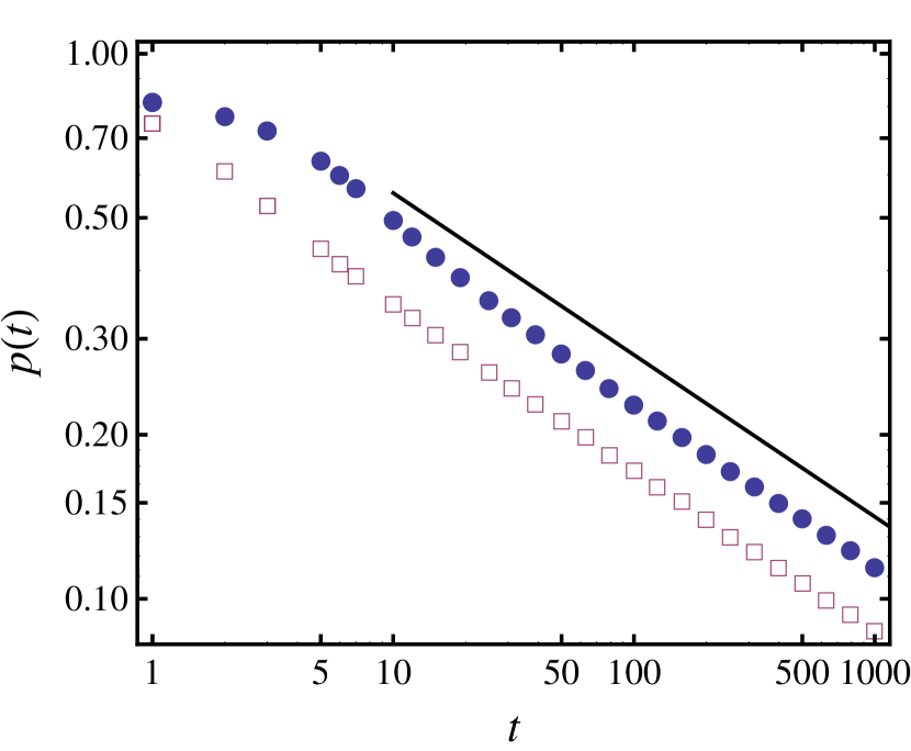
Figure 4: Persistence probability of a semi-flexible polymer in a shear flow for values of $a=0.1$ ( $\bullet$) and $0.50$ ( $\square$). The solid black line is a plot of $t^{-\theta}$, with $\theta=0.29695$, the prediction of IIA. A power law fit to the asymptotic of the data yields $\theta=0.306236$ for $a=0.1$ and $\theta=0.297205$ for $a=0.5$.

5 Conclusion

In conclusion, we have presented results for the two-time correlation functions of a single free and confined Brownian particle in a simple shear flow. The confinement of the Brownian particle is modeled as a harmonic trap, often encountered in trapping and tracking experiments. The persistence probability, defined as the probability that the sign of the stochastic observable has not changed sign up to time $t$ is constructed from the correlation function. The probability shows two distinct algebraic decays. For short times $t<<a^{-1}$, when the particle does not feel the effect of the shear, the motion is found to be purely diffusive while at late times the motion is super ballistic with the mean-square-displacement along the direction of shear scaling as $t^{3}$. We have also extended the analysis to a chain of Brownian particles interacting via a harmonic potential and a bending potential. The asymptotic of the persistence probability is found to decay as a power law with as exponent in close agreement with that of the predictions from Independent Interval Approximations.

References

- (1) S.N. Majumdar, Current Science 77, 370 (1999)
- (2) P. Ray, Phase Transitions 77(5-7), 563 (2004)
- (3) S.N. Majumdar, C. Sire, A.J. Bray, S.J. Cornell, Phys. Rev. Lett. 77, 2867 (1996)
- (4) S. Bhattacharya, D. Das, S.N. Majumdar, Phys. Rev. E 75, 061122 (2007)
- (5) C. Sire, S.N. Majumdar, A. Rüdinger, Phys. Rev. E 61, 1258 (2000)
- (6) D. Chakraborty, J.K. Bhattacharjee, Phys. Rev. E 75, 011111 (2007)
- (7) T. Newman, Z. Toroczkai, Physical Review E 58(3), R2685 (1998)
- (8) D. Chakraborty, Phys. Rev. E 79, 031112 (2009)
- (9) J. Krug, H. Kallabis, S.N. Majumdar, S.J. Cornell, A.J. Bray, C. Sire, Phys. Rev. E 56, 2702 (1997)
- (10) Z. Toroczkai, T.J. Newman, S. Das Sarma, Phys. Rev. E 60, R1115 (1999)
- (11) M. Constantin, C. Dasgupta, P.P. Chatraphorn, S.N. Majumdar, S. Das Sarma, Phys. Rev. E 69, 061608 (2004)
- (12) S.N. Majumdar, A.J. Bray, S.J. Cornell, C. Sire, Phys. Rev. Lett. 77, 3704 (1996)
- (13) M.R. Swift, A.J. Bray, Phys. Rev. E 59, R4721 (1999)
- (14) T.W. Burkhardt, Journal of Physics A: Mathematical and General 33(45), L429 (2000)
- (15) D.S. Fisher, P. Le Doussal, C. Monthus, Phys. Rev. Lett. 80, 3539 (1998)
- (16) P. Le Doussal, C. Monthus, D.S. Fisher, Phys. Rev. E 59, 4795 (1999)
- (17) D. Chakraborty, The European Physical Journal B - Condensed Matter and Complex Systems 64, 263 (2008), 10.1140/epjb/e2008-00300-1
- (18) D. Slepian, Bell System Tech. J 41(2), 463 (1962)
- (19) S.O. Rice, Bell System Tech. J 24, 46 (1945)
- (20) E. Frey, K. Kroy, Annalen der Physik 14(1-3), 20 (2005)
- (21) M.S. Miguel, J. Sancho, Physica A: Statistical Mechanics and its Applications 99(1–2), 357 (1979)
- (22) G. Taylor, Proceedings of the Royal Society of London. Series A. Mathematical and Physical Sciences 219(1137), 186 (1953)
- (23) Y. Katayama, R. Terauti, European Journal of Physics 17(3), 136 (1996)
- (24) D. Kienle, J. Bammert, W. Zimmermann, Phys. Rev. E 84, 042102 (2011)
- (25) J. Bammert, W. Zimmermann, Phys. Rev. E 82, 052102 (2010)
- (26) H. Orihara, Y. Takikawa, Phys. Rev. E 84, 061120 (2011)
- (27) T.T. Perkins, D.E. Smith, S. Chu, Science 276(5321), 2016 (1997)
- (28) A. Groisman, V. Steinberg, Nature 410(6831), 905 (2001)
- (29) A. Groisman, V. Steinberg, Nature 405(6782), 53 (2000)
- (30) A.J. Bray, S.N. Majumdar, Journal of Physics A: Mathematical and General 39(45), L625 (2006)
- (31) A.J. Bray, P. Gonos, Journal of Physics A: Mathematical and General 38(25), 5617 (2005)
- (32) A.J. Bray, P. Gonos, Journal of Physics A: Mathematical and General 37(30), L361 (2004)
- (33) S. Majumdar, A. Bray, G. Ehrhardt, Physical Review E 64(1) (2001)
- (34) Y.G. Sinai, Theoretical and Mathematical Physics 90, 219 (1992), 10.1007/BF01036528
- (35) T. Pham, P. Sunthar, J. Prakash, Journal of Non-Newtonian Fluid Mechanics 149(1-3), 9 (2008)
- (36) M. Manghi, X. Schlagberger, Y.W. Kim, R.R. Netz, Soft Matter 2(8), 653 (2006)
- (37) D.C. Morse, Macromolecules 31(20), 7030 (1998)