Measurement of Mixing and Violation in
Two-Body Decays
J. P. Lees
V. Poireau
V. Tisserand
Laboratoire d’Annecy-le-Vieux de Physique des Particules (LAPP), Université de Savoie, CNRS/IN2P3, F-74941 Annecy-Le-Vieux, France
J. Garra Tico
E. Grauges
Universitat de Barcelona, Facultat de Fisica, Departament ECM, E-08028 Barcelona, Spain
A. PalanoabINFN Sezione di Baria; Dipartimento di Fisica, Università di Barib, I-70126 Bari, Italy
G. Eigen
B. Stugu
University of Bergen, Institute of Physics, N-5007 Bergen, Norway
D. N. Brown
L. T. Kerth
Yu. G. Kolomensky
G. Lynch
Lawrence Berkeley National Laboratory and University of California, Berkeley, California 94720, USA
H. Koch
T. Schroeder
Ruhr Universität Bochum, Institut für Experimentalphysik 1, D-44780 Bochum, Germany
D. J. Asgeirsson
C. Hearty
T. S. Mattison
J. A. McKenna
R. Y. So
University of British Columbia, Vancouver, British Columbia, Canada V6T 1Z1
A. Khan
Brunel University, Uxbridge, Middlesex UB8 3PH, United Kingdom
V. E. Blinov
A. R. Buzykaev
V. P. Druzhinin
V. B. Golubev
E. A. Kravchenko
A. P. Onuchin
S. I. Serednyakov
Yu. I. Skovpen
E. P. Solodov
K. Yu. Todyshev
A. N. Yushkov
Budker Institute of Nuclear Physics, Novosibirsk 630090, Russia
M. Bondioli
D. Kirkby
A. J. Lankford
M. Mandelkern
University of California at Irvine, Irvine, California 92697, USA
H. Atmacan
J. W. Gary
F. Liu
O. Long
G. M. Vitug
University of California at Riverside, Riverside, California 92521, USA
C. Campagnari
T. M. Hong
D. Kovalskyi
J. D. Richman
C. A. West
University of California at Santa Barbara, Santa Barbara, California 93106, USA
A. M. Eisner
J. Kroseberg
W. S. Lockman
A. J. Martinez
B. A. Schumm
A. Seiden
University of California at Santa Cruz, Institute for Particle Physics, Santa Cruz, California 95064, USA
D. S. Chao
C. H. Cheng
B. Echenard
K. T. Flood
D. G. Hitlin
P. Ongmongkolkul
F. C. Porter
A. Y. Rakitin
California Institute of Technology, Pasadena, California 91125, USA
R. Andreassen
Z. Huard
B. T. Meadows
M. D. Sokoloff
L. Sun
University of Cincinnati, Cincinnati, Ohio 45221, USA
P. C. Bloom
W. T. Ford
A. Gaz
U. Nauenberg
J. G. Smith
S. R. Wagner
University of Colorado, Boulder, Colorado 80309, USA
R. Ayad
Now at the University of Tabuk, Tabuk 71491, Saudi Arabia
W. H. Toki
Colorado State University, Fort Collins, Colorado 80523, USA
B. Spaan
Technische Universität Dortmund, Fakultät Physik, D-44221 Dortmund, Germany
K. R. Schubert
R. Schwierz
Technische Universität Dresden, Institut für Kern- und Teilchenphysik, D-01062 Dresden, Germany
D. Bernard
M. Verderi
Laboratoire Leprince-Ringuet, Ecole Polytechnique, CNRS/IN2P3, F-91128 Palaiseau, France
P. J. Clark
S. Playfer
University of Edinburgh, Edinburgh EH9 3JZ, United Kingdom
D. BettoniaC. BozziaR. CalabreseabG. CibinettoabE. FioravantiabI. GarziaabE. LuppiabM. MuneratoabL. PiemonteseaV. SantoroaINFN Sezione di Ferraraa; Dipartimento di Fisica, Università di Ferrarab, I-44100 Ferrara, Italy
R. Baldini-Ferroli
A. Calcaterra
R. de Sangro
G. Finocchiaro
P. Patteri
I. M. Peruzzi
Also with Università di Perugia, Dipartimento di Fisica, Perugia, Italy
M. Piccolo
M. Rama
A. Zallo
INFN Laboratori Nazionali di Frascati, I-00044 Frascati, Italy
R. ContriabE. GuidoabM. Lo VetereabM. R. MongeabS. PassaggioaC. PatrignaniabE. RobuttiaINFN Sezione di Genovaa; Dipartimento di Fisica, Università di Genovab, I-16146 Genova, Italy
B. Bhuyan
V. Prasad
Indian Institute of Technology Guwahati, Guwahati, Assam, 781 039, India
C. L. Lee
M. Morii
Harvard University, Cambridge, Massachusetts 02138, USA
A. J. Edwards
Harvey Mudd College, Claremont, California 91711, USA
A. Adametz
U. Uwer
Universität Heidelberg, Physikalisches Institut, Philosophenweg 12, D-69120 Heidelberg, Germany
H. M. Lacker
T. Lueck
Humboldt-Universität zu Berlin, Institut für Physik, Newtonstr. 15, D-12489 Berlin, Germany
P. D. Dauncey
Imperial College London, London, SW7 2AZ, United Kingdom
U. Mallik
University of Iowa, Iowa City, Iowa 52242, USA
C. Chen
J. Cochran
W. T. Meyer
S. Prell
A. E. Rubin
Iowa State University, Ames, Iowa 50011-3160, USA
A. V. Gritsan
Z. J. Guo
Johns Hopkins University, Baltimore, Maryland 21218, USA
N. Arnaud
M. Davier
D. Derkach
G. Grosdidier
F. Le Diberder
A. M. Lutz
B. Malaescu
P. Roudeau
M. H. Schune
A. Stocchi
G. Wormser
Laboratoire de l’Accélérateur Linéaire, IN2P3/CNRS et Université Paris-Sud 11, Centre Scientifique d’Orsay, B. P. 34, F-91898 Orsay Cedex, France
D. J. Lange
D. M. Wright
Lawrence Livermore National Laboratory, Livermore, California 94550, USA
C. A. Chavez
J. P. Coleman
J. R. Fry
E. Gabathuler
D. E. Hutchcroft
D. J. Payne
C. Touramanis
University of Liverpool, Liverpool L69 7ZE, United Kingdom
A. J. Bevan
F. Di Lodovico
R. Sacco
M. Sigamani
Queen Mary, University of London, London, E1 4NS, United Kingdom
G. Cowan
University of London, Royal Holloway and Bedford New College, Egham, Surrey TW20 0EX, United Kingdom
D. N. Brown
C. L. Davis
University of Louisville, Louisville, Kentucky 40292, USA
A. G. Denig
M. Fritsch
W. Gradl
K. Griessinger
A. Hafner
E. Prencipe
Johannes Gutenberg-Universität Mainz, Institut für Kernphysik, D-55099 Mainz, Germany
R. J. Barlow
Now at the University of Huddersfield, Huddersfield HD1 3DH, UK
G. Jackson
G. D. Lafferty
University of Manchester, Manchester M13 9PL, United Kingdom
E. Behn
R. Cenci
B. Hamilton
A. Jawahery
D. A. Roberts
University of Maryland, College Park, Maryland 20742, USA
C. Dallapiccola
University of Massachusetts, Amherst, Massachusetts 01003, USA
R. Cowan
D. Dujmic
G. Sciolla
Massachusetts Institute of Technology, Laboratory for Nuclear Science, Cambridge, Massachusetts 02139, USA
R. Cheaib
D. Lindemann
P. M. Patel
S. H. Robertson
McGill University, Montréal, Québec, Canada H3A 2T8
P. BiassoniabN. NeriaF. PalomboabS. StrackaabINFN Sezione di Milanoa; Dipartimento di Fisica, Università di Milanob, I-20133 Milano, Italy
L. Cremaldi
R. Godang
Now at University of South Alabama, Mobile, Alabama 36688, USA
R. Kroeger
P. Sonnek
D. J. Summers
University of Mississippi, University, Mississippi 38677, USA
X. Nguyen
M. Simard
P. Taras
Université de Montréal, Physique des Particules, Montréal, Québec, Canada H3C 3J7
G. De NardoabD. MonorchioabG. OnoratoabC. SciaccaabINFN Sezione di Napolia; Dipartimento di Scienze Fisiche, Università di Napoli Federico IIb, I-80126 Napoli, Italy
M. Martinelli
G. Raven
NIKHEF, National Institute for Nuclear Physics and High Energy Physics, NL-1009 DB Amsterdam, The Netherlands
C. P. Jessop
J. M. LoSecco
W. F. Wang
University of Notre Dame, Notre Dame, Indiana 46556, USA
K. Honscheid
R. Kass
Ohio State University, Columbus, Ohio 43210, USA
J. Brau
R. Frey
N. B. Sinev
D. Strom
E. Torrence
University of Oregon, Eugene, Oregon 97403, USA
E. FeltresiabN. GagliardiabM. MargoniabM. MorandinaM. PosoccoaM. RotondoaG. SimiaF. SimonettoabR. StroiliabINFN Sezione di Padovaa; Dipartimento di Fisica, Università di Padovab, I-35131 Padova, Italy
S. Akar
E. Ben-Haim
M. Bomben
G. R. Bonneaud
H. Briand
G. Calderini
J. Chauveau
O. Hamon
Ph. Leruste
G. Marchiori
J. Ocariz
S. Sitt
Laboratoire de Physique Nucléaire et de Hautes Energies, IN2P3/CNRS, Université Pierre et Marie Curie-Paris6, Université Denis Diderot-Paris7, F-75252 Paris, France
M. BiasiniabE. ManoniabS. PacettiabA. RossiabINFN Sezione di Perugiaa; Dipartimento di Fisica, Università di Perugiab, I-06100 Perugia, Italy
C. AngeliniabG. BatignaniabS. BettariniabM. CarpinelliabAlso with Università di Sassari, Sassari, Italy
G. CasarosaabA. CervelliabF. FortiabM. A. GiorgiabA. LusianiacB. OberhofabE. PaoloniabA. PerezaG. RizzoabJ. J. WalshaINFN Sezione di Pisaa; Dipartimento di Fisica, Università di Pisab; Scuola Normale Superiore di Pisac, I-56127 Pisa, Italy
D. Lopes Pegna
J. Olsen
A. J. S. Smith
A. V. Telnov
Princeton University, Princeton, New Jersey 08544, USA
F. AnulliaR. FacciniabF. FerrarottoaF. FerroniabM. GasperoabL. Li GioiaM. A. MazzoniaG. PireddaaINFN Sezione di Romaa; Dipartimento di Fisica, Università di Roma La Sapienzab, I-00185 Roma, Italy
C. Bünger
O. Grünberg
T. Hartmann
T. Leddig
H. Schröder
C. Voss
R. Waldi
Universität Rostock, D-18051 Rostock, Germany
T. Adye
E. O. Olaiya
F. F. Wilson
Rutherford Appleton Laboratory, Chilton, Didcot, Oxon, OX11 0QX, United Kingdom
S. Emery
G. Hamel de Monchenault
G. Vasseur
Ch. Yèche
CEA, Irfu, SPP, Centre de Saclay, F-91191 Gif-sur-Yvette, France
D. Aston
D. J. Bard
R. Bartoldus
J. F. Benitez
C. Cartaro
M. R. Convery
J. Dorfan
G. P. Dubois-Felsmann
W. Dunwoodie
M. Ebert
R. C. Field
M. Franco Sevilla
B. G. Fulsom
A. M. Gabareen
M. T. Graham
P. Grenier
C. Hast
W. R. Innes
M. H. Kelsey
P. Kim
M. L. Kocian
D. W. G. S. Leith
P. Lewis
B. Lindquist
S. Luitz
V. Luth
H. L. Lynch
D. B. MacFarlane
D. R. Muller
H. Neal
S. Nelson
M. Perl
T. Pulliam
B. N. Ratcliff
A. Roodman
A. A. Salnikov
R. H. Schindler
A. Snyder
D. Su
M. K. Sullivan
J. Va’vra
A. P. Wagner
W. J. Wisniewski
M. Wittgen
D. H. Wright
H. W. Wulsin
C. C. Young
V. Ziegler
SLAC National Accelerator Laboratory, Stanford, California 94309 USA
W. Park
M. V. Purohit
R. M. White
J. R. Wilson
University of South Carolina, Columbia, South Carolina 29208, USA
A. Randle-Conde
S. J. Sekula
Southern Methodist University, Dallas, Texas 75275, USA
M. Bellis
P. R. Burchat
T. S. Miyashita
E. M. T. Puccio
Stanford University, Stanford, California 94305-4060, USA
M. S. Alam
J. A. Ernst
State University of New York, Albany, New York 12222, USA
R. Gorodeisky
N. Guttman
D. R. Peimer
A. Soffer
Tel Aviv University, School of Physics and Astronomy, Tel Aviv, 69978, Israel
P. Lund
S. M. Spanier
University of Tennessee, Knoxville, Tennessee 37996, USA
J. L. Ritchie
A. M. Ruland
R. F. Schwitters
B. C. Wray
University of Texas at Austin, Austin, Texas 78712, USA
J. M. Izen
X. C. Lou
University of Texas at Dallas, Richardson, Texas 75083, USA
F. BianchiabD. GambaabS. ZambitoabINFN Sezione di Torinoa; Dipartimento di Fisica Sperimentale, Università di Torinob, I-10125 Torino, Italy
L. LanceriabL. VitaleabINFN Sezione di Triestea; Dipartimento di Fisica, Università di Triesteb, I-34127 Trieste, Italy
F. Martinez-Vidal
A. Oyanguren
IFIC, Universitat de Valencia-CSIC, E-46071 Valencia, Spain
H. Ahmed
J. Albert
Sw. Banerjee
F. U. Bernlochner
H. H. F. Choi
G. J. King
R. Kowalewski
M. J. Lewczuk
I. M. Nugent
J. M. Roney
R. J. Sobie
N. Tasneem
University of Victoria, Victoria, British Columbia, Canada V8W 3P6
T. J. Gershon
P. F. Harrison
T. E. Latham
Department of Physics, University of Warwick, Coventry CV4 7AL, United Kingdom
H. R. Band
S. Dasu
Y. Pan
R. Prepost
S. L. Wu
University of Wisconsin, Madison, Wisconsin 53706, USA
Abstract
We present a measurement of mixing and violation
using the ratio of lifetimes simultaneously extracted from
a sample of mesons produced through the flavor-tagged
process , where decays to ,
, or , along with the untagged decays
and . The lifetimes of the
-even, Cabibbo-suppressed modes and are
compared to that of the -mixed mode in order to measure and .
We obtain
and
,
where constrains possible violation.
The result excludes the null mixing hypothesis at significance.
This analysis is based on an integrated luminosity of
collected with the BABAR detector at the PEP-II asymmetric-energy
collider.
One manifestation of mixing is differing decay time
distributions for decays to different eigenstates Liu:1994ea .
We present a measurement of charm mixing using the ratio of lifetimes obtained from the decays of neutral mesons to -even
and -mixed two-body final states.
We also present a search for indirect violation arising from a difference in and partial decay widths to -even
eigenstates. Recently the LHCb Collaboration has reported evidence for in the difference of the time-integrated asymmetries
in and decays Aaij:2011in .
This measurement is primarily sensitive to direct .
As explained in Appendix A, we are not sensitive to effects of direct violation at the level of the result reported by LHCb,
and we therefore assume no direct in our baseline model.
We measure the effective lifetimes in three different
two-body final states: , , and .
We make no distinction between the
Cabibbo-favored and doubly Cabibbo-suppressed
modes; in other words, we analyze and describe them together.
Given the current experimental evidence indicating a small mixing rate,
the lifetime distribution for all two-body final states is exponential
to a good approximation.
Decays in the mode are to a -mixed final state, and are
assumed to be described by the average width .
The singly Cabibbo-suppressed decays () to the -even and
final states are described by the partial decay rate (),
where indicates the of the final state.
We present in Appendix A a discussion of the
mixing formalism leading to the expressions that
are used to extract the mixing parameter and the
parameter ,
(1)
(2)
from the experimentally measured -mixed and -even lifetimes.
This definition of is opposite in sign to that in our previous measurement Aubert:2007en and is now consistent with that used by the Heavy Flavor Averaging Group Asner:2010qj .
We use mesons from tagged
decays CC:2008 , as well as untagged decays where
no parent is found.
The charge of the is used to split the and samples into those originating from and from mesons in order to measure the -violating parameter .
The requirement of a parent strongly suppresses backgrounds; hence untagged decays are reconstructed only in and because of the relatively poor signal-to-background ratio in the untagged final state.
In summary we study seven modes, two untagged and five tagged.
In addition to the increased integrated luminosity of the new dataset compared to that used in our earlier results Aubert:2007en ; Aubert:2009ai ,
this analysis benefits from improved particle identification and charged-particle track reconstruction, and a more inclusive and optimized event selection.
We implement an improved background model, and we simultaneously fit both the tagged and untagged datasets.
II Event Reconstruction and Selection
We use of colliding-beam data recorded at, and slightly
below, the resonance ( center-of-mass [CM] energy )
with the BABAR detector Aubert:2001tu
at the SLAC National Accelerator Laboratory PEP-II asymmetric-energy Factory.
To avoid potential bias, we finalize our data selection criteria,
as well as the procedures for fitting, extracting statistical limits,
and determining systematic uncertainties, prior to examining the results.
We reconstruct charged tracks and vertices with a 5-layer, double-sided silicon vertex tracker (SVT)
and a 40-layer drift chamber (DCH). We select candidates by pairing oppositely charged tracks,
requiring each track to satisfy particle identification criteria based on specific ionization energy loss ()
from the SVT and DCH, and Cherenkov angle measurements from a ring-imaging Cherenkov detector (DIRC).
We then refit the daughter tracks, requiring them to originate from a common vertex.
To reduce contributions from ’s
produced via -meson decay to a negligible level,
we require each to have momentum in the CM frame .
For tagged decays, we reconstruct candidates by combining a candidate with a
slow pion track , requiring them to originate
from a common vertex constrained to the interaction region.
We require the momentum
to be greater than in the laboratory frame and less than
in the CM frame.
We reject a positron that fakes a candidate
by using information and veto
any candidate that may have originated from a reconstructed
photon conversion or Dalitz decay.
The distribution of the difference between the reconstructed and
masses peaks near . Backgrounds are
suppressed by retaining only tagged candidates in the range .
To determine the proper time and its error for each candidate,
we perform a combined fit to the production and decay vertices. We constrain the
production point to be within the interaction region, which we
determine using Bhabha and di-muon events from triggers close in time to any given signal candidate event.
We retain only candidates with a -based probability
for the fit , and with
and .
For tagged decays, this fit does not
incorporate any information in order
to ensure that the lifetime resolution models for tagged and untagged
signal decays are very similar.
The most probable value of for signal events
is of the nominal lifetime Nakamura:2010zzi .
If an event contains a tagged decay, we exclude all untagged candidates from that event in the final sample.
For a given final state, when multiple (for the untagged modes) or (for the tagged modes)
candidates in an event share one or more tracks, we retain only the candidate with the highest
. The fraction of events with multiple candidates with overlapping
daughter tracks is for all final states.
III Invariant Mass Fits
We characterize the invariant mass () distribution for each of the seven modes with an extended unbinned
maximum likelihood fit to and samples.
We allow the parameters governing the shapes of the probability density functions (PDFs),
as well as the expected signal and background candidate yields, to vary in the fits.
For the tagged -even modes we fit the and samples simultaneously, sharing all parameters except for the
expected signal and background candidate yields.
We fit the tagged invariant mass distribution in the fit range
using a sum of two Gaussians with independent means and widths for the signal PDF,
along with a first-order Chebychev polynomial for the total background.
The fit model for the tagged invariant mass distribution is similar to ,
except that the fit range is ,
and the signal PDF is the sum of two independent Gaussians
and a modified Gaussian with a power-law tail Oreglia:1980cs , which aids in better modeling of
the lower tail of the distribution.
The signal PDF for the untagged mode and for both tagged and untagged modes is a sum of three independent Gaussians;
the background is modeled using a second-order Chebychev polynomial.
The mass fit range is for the untagged mode, for the untagged mode, and for the tagged mode.
In these modes, we do not distinguish from candidates, and therefore determine
only the total signal and total background yields, in addition to the signal and background shape parameters.
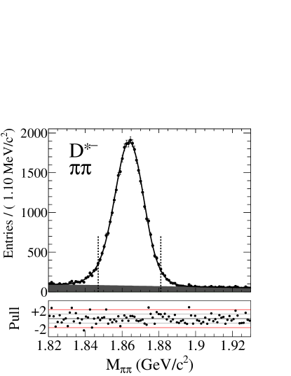
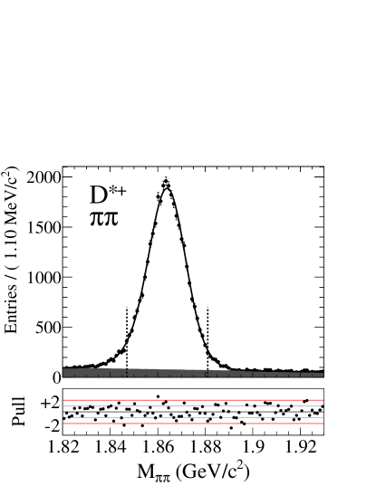
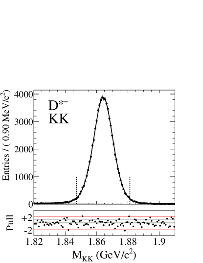
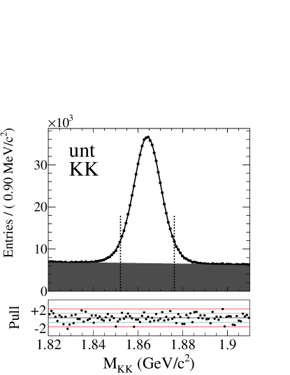
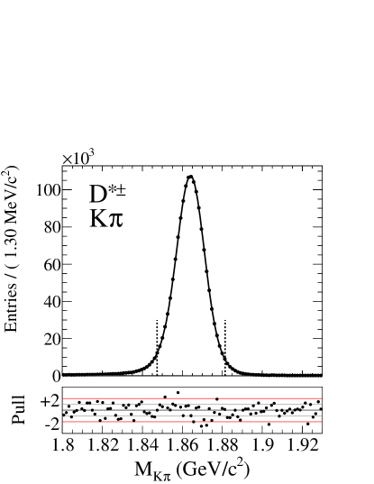
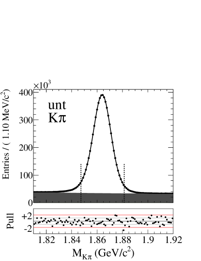
The reconstructed invariant mass distributions and the fit results are shown in Fig. 1,
together with a plot of the corresponding normalized Poisson pulls Baker:1983tu .
Figure 1: The reconstructed two-body invariant mass distributions
for the seven modes. The vertical lines show the lifetime-fit mass
region, defined in Sec. IV. The shaded regions are the background contributions.
The normalized Poisson pulls for each fit are shown under each plot; “unt” refers to the untagged datasets.
IV Signal and Sideband Regions
For the lifetime fit, we determine the regions in two-body invariant
mass that maximize signal significance, minimize systematic effects due
to backgrounds, and minimize the effect of the correlation between invariant mass and proper time.
We refer to these regions as the lifetime-fit mass regions.
Based on these studies, the optimal
lifetime-fit mass region is wide for all tagged modes
and untagged events, .
Because of the smaller signal-to-background ratio for the
untagged events, the lifetime-fit mass region for this
mode is only in width, .
For the tagged modes, a mass difference
sideband is used, along with a low (high)
invariant mass sideband, .
The low (high) mass sideband used for the untagged modes, , is displaced from the tagged sideband
in order to reduce the signal component there.
The signal purities in the lifetime-fit mass regions range from for the
untagged sample to for the tagged events.
We classify candidate decays in the lifetime-fit mass region as follows:
signal decays; misreconstructed-charm decays, i.e., those in which the candidate- daughter tracks are
decay products of a non-signal weak charm decay; and random combinatorial background.
Table 1 gives the composition of the
misreconstructed-charm backgrounds expected from simulated events simulation in each final state.
Table 1: Expected composition (in %) of the misreconstructed-charm backgrounds.
Only misreconstructed-charm background
channels that have contribution in at least one signal mode are listed.
For the tagged modes, the yields are the sum of the separate and tags.
Mode
Tagged Modes
Untagged Modes
15.4
10.3
29.9
7.2
80.8
14.9
57.1
8.8
35.8
1.1
70.3
1.7
63.3
6.9
2.9
11.8
1.3
3.5
1.8
2.2
3.1
7.0
17.3
decays
4.9
2.6
V lifetime fit
The lifetimes are determined from an extended unbinned maximum likelihood fit
to and for candidates in the lifetime-fit mass region. All modes are
fit simultaneously using shared signal resolution function parameters.
The signal, misreconstructed-charm and combinatorial components are described by their own set of PDFs,
which in the tagged modes can also depend on the charm flavor.
The lifetime PDF for signal is an exponential function convolved with a resolution function,
which is the sum of three Gaussian functions whose widths are
proportional to .
The explicit form of the signal lifetime PDF is
where (with )
parameterizes the contribution of each individual Gaussian,
(with ) is a scaling factor associated with each Gaussian, and
is an offset of the mean of the resolution function. The function
is given by
(4)
where the normalization coefficient is chosen such that
(5)
With this definition, the product
is a properly normalized two-dimensional conditional PDF, where () is a
PDF characterizing the distribution, described below.
To account for small differences in the resolution function for the different final states
we introduce additional mode-dependent scale factors , .
We also allow for differences between the resolution functions for tagged and untagged modes
by means of scale factors , tag (tagged) or unt (untagged).
We fix and to 1.
The three lifetime parameters are , where is extracted from the tagged and untagged
modes, while and are extracted from the tagged and untagged -even modes.
Approximately 0.4% of the tagged -even samples contain correctly reconstructed candidates combined
with an unrelated ; this fraction has been estimated from simulated
events and verified in data by an earlier BABAR analysis Aubert:2007wf .
These candidates have the same resolution and lifetime behavior as those from correctly reconstructed decays,
but about half of them will be tagged as the wrong flavor. Therefore, the tagged -even proper-time distributions
are modeled as the weighted sum of PDFs for correctly tagged and untagged candidates, characterized by the lifetime parameters
and , respectively, and a mistag fraction .
The tagged -even proper-time distributions are modeled in a similar fashion, where now the correctly tagged and mistagged PDFs are characterized by the lifetime parameters and , respectively.
The untagged proper-time distribution is modeled as a weighted sum of two PDFs characterized by the lifetime parameters and ,
respectively, and a weighting fraction .
These parameterizations assume no direct , and allow for in the interference between decays with and without mixing characterized by a mode-independent weak phase .
Both and are varied as part of the systematic error estimate for and .
All five tagged and two untagged signal lifetime PDFs are explicitly given in Appendix B.
The PDF for signal candidates is obtained directly
from data by subtracting the sum of the background distributions from
that of all candidates in the lifetime-fit mass region.
These 1-d distributions are used to model the
PDF discussed previously.
We determine the versus misreconstructed-charm signal-like PDF shape parameters and yields
by fitting simulated events in the lifetime-fit mass region and then fix these parameters in the lifetime fit to data.
We vary the lifetimes and yields as part of the study of systematic effects.
The largest background in the lifetime-fit mass region is due to random combinations of tracks.
The PDF describing the two-dimensional combinatorial background in and in the
lifetime-fit mass region is characterized as a weighted average of the 2-d PDFs extracted
from the mass sideband regions.
The weights for the low and high sidebands are obtained from simulated events.
The combinatorial PDF in each sideband and for each mode, except for the untagged mode, is extracted as a 2-d histogram from the sideband samples. From
these histograms we subtract the contribution of signal and
misreconstructed-charm backgrounds, each of which is estimated from
simulated events, to obtain the final combinatorial PDF in each sideband.
For the untagged mode, a similar procedure is used but, instead of
histograms, analytic signal-like PDFs are used.
For the background PDFs the offsets and the lifetimes are allowed to be different
for each Gaussian.
The signal and misreconstructed-charm PDF parameters are extracted by fitting simulated
events and then fixed, along with the expected candidate yields, in the fit that extracts the combinatorial PDFs in each sideband.
For the untagged mode both the expected signal and combinatorial yields
are free parameters in the lifetime fit.
The expected combinatorial background yields in the other modes are
determined by integrating the total background PDF extracted from the mass fit in the lifetime-fit
mass region, and then subtracting the expected misreconstructed-charm background yields, which are determined from samples of simulated events.
A small bias on these fit yields is observed in fits to
simulated events. To correct for this, we scale the data yields based on
the simulated-event fits and vary the mode-dependent scale factors as a systematic uncertainty.
Table 2 gives the event class yields plus uncertainties obtained from the lifetime fit
and indicates the yields that are fixed.
Table 2: Signal and background yields in the lifetime-fit mass region. Yields with
uncertainties are those obtained directly from the lifetime fit to data. For the tagged modes,
the yields are the sum of the separate and tags.
Tagged Modes
Untagged Modes
Signal
Comb. Bkgd.
3760
653
2849
Charm Bkgd.
97
309
642
5477
4645
The simultaneous fit to all events in the lifetime-fit mass region
has 20 floating parameters: the seven signal yields and three signal lifetimes;
the yield of untagged combinatorial candidates; the offset ;
the parameters and characterizing the weight of each Gaussian in the signal resolution mode;
and the proper-time error scaling parameters , and .
After extracting the three signal lifetimes, using their
reciprocals in the computation of and as
defined in Eqs. (1) and (2), respectively, we find
The statistical errors are computed using the covariance matrix returned by the fit.
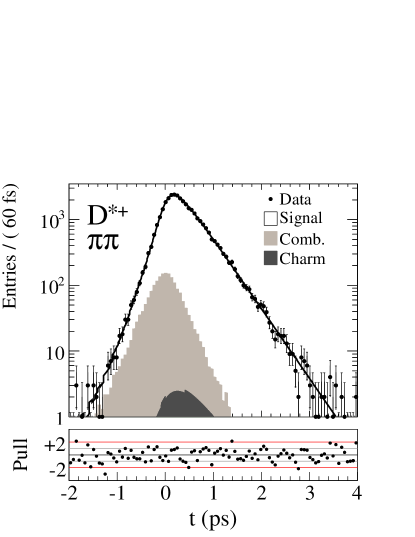
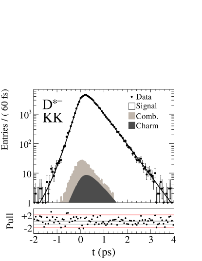
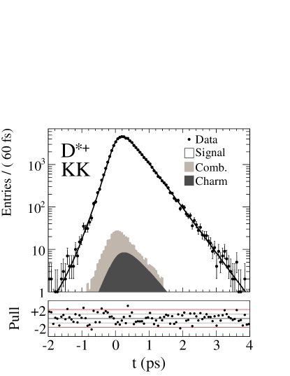
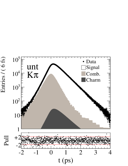
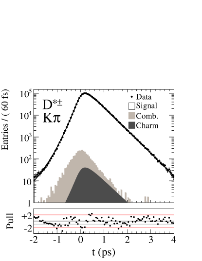
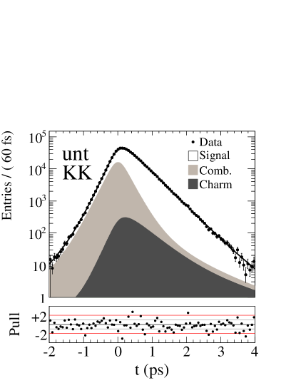
The lifetime-fit mass region proper-time distributions and projections of the lifetime fit
for the seven different decay modes are shown in Fig. 2.
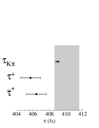
Figure 2: Proper-time distribution for each decay mode with the fit results overlaid.
The combinatorial distribution (indicated as ‘Comb.’ in light gray) is stacked on top of the misreconstructed-charm
distribution (indicated as ‘Charm’ in dark gray).
The normalized Poisson pulls for each fit are shown under each plot; “unt” refers to the untagged datasets.
The bottom right plot shows the individual lifetimes (with statistical uncertainties only);
the gray band indicates the PDG lifetime Nakamura:2010zzi .
VI cross checks and systematics
We have performed numerous cross checks to search
for potential problems, in addition to quantitative studies
that yield the systematic uncertainties given in
Table 3, discussed below.
Initially we tested the fit model by generating large ensembles of
datasets randomly drawn from the underlying total PDF, and observed no biases in the and
results obtained.
In addition, we have fit an ensemble of four simulated datasets, each equivalent in luminosity to the data,
and found no evidence of bias in or .
In fitting the data, we find that the tagged and untagged extracted lifetimes for , and separately for ,
are compatible within the statistical uncertainties.
We performed a simultaneous fit to the tagged channels, and a separate simultaneous fit to the untagged channels, and find the lifetimes
to be compatible within the statistical uncertainties.
We repeated the fit allowing the and final states to have separate and
lifetimes, and observed no statistically significant difference between the and
results. We estimated the effects of the SVT misalignment to be negligible.
We varied the lifetime-fit mass region width by and .
We adopt as the systematic uncertainty half the RMS of the differences
and from the nominal fit central values.
We also shifted the position of each mass region by centering each of them at
the most probable value for the signal PDF obtained in the invariant mass fits.
These systematic uncertainties are given in the first two lines of Table 3.
For the untagged mode, the combinatorial yield is a parameter determined in the lifetime fit.
However, it is also needed to determine the signal PDF. We first
use the total background yield determined from the mass fit to extract a signal PDF, which is employed in an initial simultaneous
lifetime fit. The combinatorial yield from this fit is used to construct an improved signal PDF
and a second fit is performed (the nominal fit). We estimate the systematic error on and associated
with the determination of the signal PDF for the untagged mode
to be the difference in the values obtained from an additional iteration of the fit and the nominal fit.
We vary the nominal mistag rate of by ,
a relative variation, and find no significant change in the nominal fit values.
Instead of assuming equal fractions of and in the untagged
mode, we adopt the latest CDF result for direct Aaltonen:2011se ,
and find negligible change in and .
We rely on simulated events to determine both the PDF shapes and yields
for the misreconstructed-charm backgrounds. To account for the model
dependence, we vary the effective lifetime of these events
by , except for the tagged mode where the variation is
due to the small number of simulated events that pass the selection criteria for this mode.
We also vary the expected misreconstructed-charm yields by in the
tagged channels, and in the untagged channels. Each variation is
simultaneously applied to all modes. These are variations
relative to the statistical uncertainties of the simulated datasets.
We vary the yields, weighting parameters, and fitting strategy used
to obtain the 2-d lifetime PDF for combinatorial-background events in the lifetime-fit mass region
from the mass sidebands. The yields for the tagged combinatorial-background events are varied by in the mode,
in tagged , and in .
The untagged combinatorial-background yield is varied using the value extracted from
an alternative lifetime-fit model in which the yield is allowed to vary.
The weights given to the low- and high-mass sidebands in the data in order to derive the combinatorial PDF
in the lifetime-fit mass region in data are extracted from simulated events.
They are varied by plus and minus the statistical uncertainty derived from splitting the
simulated dataset, which is equivalent to several times the nominal integrated luminosity,
into datasets that numerically match the nominal luminosity.
We also apply the variations described above for the misreconstructed-charm
background to vary the yields and shape of the PDF that describe the residual signal events in the sidebands.
This is also done for the misreconstructed-charm PDF used in the sideband fits from which the 2-d combinatorial
PDF is extracted. This yields the combinatorial PDF shape variation, which is
then used in the nominal fit, to obtain the variation reported in Table 3.
Finally, we vary the criteria by from the nominal ,
and take as the systematic uncertainty the RMS of the deviations from the nominal fit central value divided by .
We also consider two variations in how multiple candidates sharing one or more daughter tracks are treated.
In the first variation, we retain all multiple candidates, if each candidate passes all the
other selection criteria. In the second variation, we reject all multiple candidates sharing one
or more daughter tracks.
We fit these datasets using the nominal fit model, and assign the largest observed
deviation from the nominal and central values as the systematic uncertainty
in Table 3.
The total and systematic uncertainties are calculated by summing the contributions
from all sources in quadrature, and are reported in the last row of Table 3.
Table 3: The and systematic uncertainties.
The total is the sum-in-quadrature of the entries in each column.
Fit Variation
(%)
(%)
mass window width
0.057
0.022
mass window position
0.005
0.001
untagged signal PDF
0.022
0.000
mistag fraction
0.000
0.000
untagged fraction
0.001
0.000
charm bkgd. lifetimes
0.042
0.001
charm bkgd. yields
0.016
0.000
comb. yields
0.043
0.002
comb. sideband weights
0.004
0.001
comb. PDF shape
0.066
0.000
selection
0.052
0.053
candidate selection
0.028
0.011
Total
0.124
0.058
VII Conclusions
In summary, we measured and to a precision significantly better than our previous
measurements Aubert:2007en ; Aubert:2009ai .
Both results are more precise than, and consistent with, the weighted average of all previous measurements Asner:2010qj ,
when the previous BABAR results are excluded. In particular, the measurement is the most precise single measurement to date.
We obtain
We exclude the null mixing hypothesis at significance,
and find no evidence for .
Our results are consistent with the world average value of the mixing parameter
obtained from (where ) Asner:2010qj , as expected in absence of .
The value of obtained here is consistent with our previously published result Aubert:2007en
when the same definition is used in both cases.
The new value is consistent with our previous result Aubert:2009ai with a probability of
, assuming that the systematics for both the old and new
measurements are fully correlated, and taking into account the fact that of
the events in the current sample are also present in the samples used in the previous measurements Aubert:2007en ; Aubert:2009ai .
The results here supersede the previous BABAR results
for these modes Aubert:2007en ; Aubert:2009ai .
Acknowledgments
We are grateful for the
extraordinary contributions of our PEP-II colleagues in
achieving the excellent luminosity and machine conditions
that have made this work possible.
The success of this project also relies critically on the
expertise and dedication of the computing organizations that
support BABAR.
The collaborating institutions wish to thank
SLAC for its support and the kind hospitality extended to them.
This work is supported by the
US Department of Energy
and National Science Foundation, the
Natural Sciences and Engineering Research Council (Canada),
the Commissariat à l’Energie Atomique and
Institut National de Physique Nucléaire et de Physique des Particules
(France), the
Bundesministerium für Bildung und Forschung and
Deutsche Forschungsgemeinschaft
(Germany), the
Istituto Nazionale di Fisica Nucleare (Italy),
the Foundation for Fundamental Research on Matter (The Netherlands),
the Research Council of Norway, the
Ministry of Education and Science of the Russian Federation,
Ministerio de Ciencia e Innovación (Spain), and the
Science and Technology Facilities Council (United Kingdom).
Individuals have received support from
the Marie-Curie IEF program (European Union) and the A. P. Sloan Foundation (USA).
References
(1)
B. Aubert et al. (BABAR Collaboration),
Phys. Rev. Lett. 98, 211802 (2007).
(2)
B. Aubert et al. (BABAR Collaboration),
Phys. Rev. D 78, 011105 (2008).
(3)
B. Aubert et al. (BABAR Collaboration),
Phys. Rev. D 80, 071103 (2009).
(4)
M. Staric et al. (Belle Collaboration),
Phys. Rev. Lett. 98, 211803 (2007).
(5)
L. M. Zhang et al. (Belle Collaboration),
Phys. Rev. Lett. 99, 131803 (2007).
(6)
T. Aaltonen et al. (CDF Collaboration),
Phys. Rev. Lett. 100, 121802 (2008).
(7)
L. Wolfenstein,
Phys. Lett. B 164, 170 (1985).
(8)
J. F. Donoghue, E. Golowich, B. R. Holstein, and J. Trampetic,
Phys. Rev. D 33, 179 (1986).
(9)
I. I. Bigi and N. G. Uraltsev,
Nucl. Phys. B 592, 92 (2001).
(10)
A. F. Falk, Y. Grossman, Z. Ligeti, and A. A. Petrov,
Phys. Rev. D 65, 054034 (2002).
(11)
A. F. Falk et al.
Phys. Rev. D 69, 114021 (2004).
(12)
G. Burdman and I. Shipsey,
Ann. Rev. Nucl. Part. Sci. 53, 431 (2003).
(13)
A. A. Petrov,
Int. J. Mod. Phys. A 21, 5686 (2006).
(14)
E. Golowich, S. Pakvasa, and A. A. Petrov,
Phys. Rev. Lett. 98, 181801 (2007).
(15)
E. Golowich et al.
Phys. Rev. D 76, 095009 (2007).
(16)
E. Golowich et al.
Phys. Rev. D 79, 114030 (2009).
(17)
G. Blaylock, A. Seiden, and Y. Nir,
Phys. Lett. B 355, 555 (1995).
(18)
G. Isidori et al.
Phys. Lett. B 711, 46 (2012).
(19)
Y. Hochberg and Y. Nir,
arXiv:1112.5268 [hep-ph].
(20)
H. -Y. Cheng and C. -W. Chiang,
Phys. Rev. D 85, 034036 (2012).
(21)
G. F. Giudice, G. Isidori, and P. Paradisi,
JHEP 1204, 060 (2012)
(22)
T. Liu, Workshop on the Future of High Sensitivity Charm Experiments: CHARM2000, Batavia, IL, 7-9 Jun 1994
[arXiv:hep-ph/9408330].
(23)
R. Aaij et al. (LHCb Collaboration),
Phys. Rev. Lett. 108, 111602 (2012).
(24)
D. Asner et al. (HFAG Collaboration),
arXiv:1010.1589 [hep-ex].
(25)
Charge conjugation is implied throughout.
(26)
B. Aubert et al. (BABAR Collaboration),
Nucl. Instrum. Meth. A 479, 1 (2002).
(27)
K. Nakamura et al. (Particle Data Group),
J. Phys. G 37, 075021 (2010).
(29)
S. Baker and R. D. Cousins,
Nucl. Instrum. Meth. 221, 437 (1984).
(30)The detector simulation is based on the GEANT 4Agostinelli:2002hh toolkit.
The simulated events are reconstructed using the same procedure as for real data.
(31)
S. Agostinelli et al. (GEANT4 Collaboration),
Nucl. Instrum. Meth. A 506, 250 (2003).
(32)
T. Aaltonen et al. (CDF Collaboration),
Phys. Rev. D 85, 012009 (2012).
(33)
H. N. Nelson,
hep-ex/9908021.
(34)
S. Bergmann, Y. Grossman, Z. Ligeti, Y. Nir, and A. A. Petrov,
Phys. Lett. B 486, 418 (2000).
(35)
A. L. Kagan and M. D. Sokoloff,
Phys. Rev. D 80, 076008 (2009).
Appendix A Mixing Formalism and Considerations on the Role of Direct Violation
The time evolution of the flavor eigenstates and is governed by the Schrödinger equation:
The mass eigenstates and are obtained from the diagonalization of the effective Hamiltonian
.
Under the hypothesis of conservation the two mass eigenstates can be written in terms of the flavor eigenstates as
(6)
where
(7)
We choose the positive root for ; choosing the negative one just means exchanging with .
If , in case of no ,
is the -even state and the -odd state.
It is traditional to quantify the size of mixing
in terms of the parameters and
, where
() is the difference in
mass (width) of the states defined in Eq. 6
and is the average width.
If either or is non-zero, mixing will occur.
While most Standard Model expectations for the size of both are
Falk:2001hx ; Nelson:1999fgSupp , values as high as
or even higher are predicted by certain models Petrov:2006nc ; Golowich:2007ka .
violation can manifest in decays in three ways:
•
in decay, when ,
•
in mixing, when ,
•
in the interference between decays with and without mixing, when the weak phase of is different from zero,
where () is the amplitude for () decaying into a final state ,
().
The presence of mixing alters the exponential distribution for the decay into a final state . In particular we have
In this analysis we are interested in -even final states ().
If we neglect second-order terms in and , the decay
time distributions can be treated as exponentials with effective widths Bergmann:2000idSupp :
(10)
(11)
To better understand the effects of violation we introduce two more parameters, one describing in decay () and one in mixing ():
(12)
(13)
Since then .
Noting that there is no strong phase in since the final state is its own -conjugate,
we can express in terms of , and the -violating phase :
(14)
Expanding Eqs. 10 and 11, and retaining only terms up to first order in and , we obtain
Combining the widths defined above we obtain the two observables and , which,
in general, depend on the final state because of the parameters and :
(17)
(18)
Other experiments characterize the -violating observable as ,
(19)
The relationship between , and is
(20)
These quantities are directly related to the fundamental parameters that govern mixing and in the charm sector:
(21)
(22)
Both and are zero if there is no mixing. Otherwise,
a non-zero value of implies mixing and a non-zero value of implies .
In the charm sector, because the CKM elements involved belong to the Cabibbo submatrix,
we can assume that the weak phase does not depend
on the final state: Kagan:2009gb . As stated earlier if direct has a
significant effect, then the values of and depend on the final state.
In this analysis we assume that the effect of direct is negligible in the
decays to eigenstates; i.e., we assume
(and ).
In Eqs. A and A this means neglecting
the linear terms in .
Assuming that and are both and ,
the neglected term is , beyond any current experimental sensitivity.