Thermal Casimir effect in the interaction of graphene with dielectrics and metals

Abstract

We investigate the thermal Casimir interaction of a suspended graphene described by the Dirac model with a plate made of dielectric or metallic materials. The reflection coefficients on graphene expressed in terms of a temperature-dependent polarization tensor are used. We demonstrate that for a graphene with nonzero mass gap parameter the Casimir free energy remains nearly constant (and the thermal correction negligibly small) over some temperature interval. For the interaction of graphene with metallic plate, the free energy is nearly the same, irrespective of whether the metal is nonmagnetic or magnetic and whether it is described using the Drude- or plasma-model approaches. The free energy computed using the Dirac model was compared with that computed using the hydrodynamic model of graphene and big differences accessible for experimental observation have been found. For dielectric and nonmagnetic metallic plates described by the Drude model these differences vanish with increasing temperature (separation). However, for nonmagnetic metals described by the plasma model and for magnetic metals, a severe dependence on the chosen theoretical description of graphene remains even at high temperature. In all cases the analytic asymptotic expressions for the free energy at high temperature are obtained and found in a very good agreement with the results of numerical computations.

I Introduction

It has been known that nanostructures based on carbon possess unique mechanical, electrical and optical properties.1 Among them particular attention has been given to graphene, a two-dimensional sheet of carbon atoms arranged in a hexagonal structure with low-energy electronic excitations described by the Dirac equation.2 At the present time suspended graphene membranes up to $55\,\mu$m diameter are produced.3 This makes possible to investigate the van der Waals and Casimir interaction between graphene and different material structures, such as another sheet of graphene, atoms, molecules, dielectric and metallic plates, spheres etc. Respective theoretical investigations were performed using the phenomenological density-functional methods,4 ; 5 ; 6 ; 7 ; 8 second-order perturbation theory9 and, for multilayered carbon nanostructures, using the Lifshitz theory.10

To apply the Lifshitz theory, one needs the reflection coefficients on graphene over a wide frequency region. It is customary to express the reflection coefficients in terms of the frequency-dependent dielectric permittivity, a concept which is not well defined for one-atom-thick carbon nanostructures. Because of this, two models for the reflection coefficients on graphene with no use of dielectric permittivity were proposed, the hydrodynamic one11 ; 12 and the Dirac one.13 ; 14 In the framework of the hydrodynamic model, graphene is considered as an infinitesimally thin positively charged sheet, carrying a homogeneous fluid with some mass and negative charge densities. The hydrodynamic model was applied for calculation of the Casimir and Casimir-Polder interactions.15 ; 16 ; 17 In the framework of the Dirac model, it is taken into account that for energies below a few eV the dispersion relation for quasiparticles in graphene is linear with respect to the momentum, whereas it is quadratic in the hydrodynamic model. The reflection coefficients of graphene at zero and nonzero temperature were found in Refs. 18 and 19 , respectively. Some calculations of the Casimir-Polder graphene-atom interaction were performed at zero temperature using both the hydrodynamic and Dirac models.20 ; 21 It should be remembered, however, that both these models are only approximations. As was already mentioned, the hydrodynamic model disregards the Dirac character of charge carriers in graphene. As to the Dirac model, it extends the linear dispersion relation for quasiparticles to any energy, whereas this property applies only at low energies. Because of this, one can conclude that in calculations of the Casimir and Casimir-Polder forces the Dirac model of graphene should be applicable at large separations between the test bodies, whereas the hydrodynamic model might work at short separation distances.

There is also another approach to the application of the Lifshitz theory to graphene. In this approach graphene is characterized by a spatially nonlocal dielectric permittivity depending both on the frequency and the wave vector. Different authors express such a dielectric permittivity either through the polarizability of one graphene layer 21a or in the random phase approximation.21b

It is well known that thermal Casimir effect is a subject of debate and there are different theoretical approaches to its description.22 ; 23 ; 24 For two graphene sheets in a nonretarded regime it was found25 that a relatively large thermal correction to the Casimir force at room temperature arises at short separation distances of tens of nanometers. This conclusion was qualitatively confirmed,19 using the Dirac model of graphene, with an alternative explanation. The reason for the origin of large thermal correction for graphene is that the contribution of all terms with nonzero Matsubara frequencies at room temperature becomes small in comparison with the zero-frequency term even at short separations. It was also found26 that in graphene-atom Casimir-Polder interaction the thermal effect depends crucially on the magnitude of a mass gap parameter in the Dirac model. Specifically, for a nonzero gap there exists an interval of temperatures (separations) where the thermal correction remains small with increasing temperature (separation). The possibility of large thermal correction at short separations links the Dirac model of graphene to the Drude model used in the literature to describe the Casimir effect between real metals.23 ; 24 Because of this, it is of much interest to investigate the thermal Casimir effect in the interaction of graphene with real material bodies made of different materials.

In this paper, we calculate the free energy of the Casimir interaction between a suspended graphene membrane described by the Dirac model and dielectric (silicon, sapphire) or metallic (Au, Ni) plates. In so doing materials of the plate are described by realistic dielectric permittivities taking into account the interband transitions of core electrons. We demonstrate that, similar to graphene-atom interaction, the behavior of thermal correction crucially depends on the mass gap parameter $\Delta$ of the Dirac model. Note that although the Dirac-type excitations in pristine graphene are gapless, the influence of electron-electron interaction, substrates, defects of structure, and other effects leads to a nonzero mass gap.2 ; 26a ; 26b ; 26c ; 26d Specifically, we show that larger is the magnitude of mass gap parameter, wider is the separation (temperature) interval, where the thermal correction remains small with increasing separation (temperature). For a metallic plate interacting with graphene, we perform all calculations using both the Drude- and plasma-model approaches to the dielectric permittivity of metal. In the case when graphene described by the Dirac model interacts with a metallic plate (either nonmagnetic or magnetic) the calculation results obtained using both approaches nearly coincide and do not depend on the magnetic properties. In contrast to the case of two Drude metals, the thermal correction for a graphene-metal interaction has the same sign as the interaction energy at zero temperature, i.e., the magnitude of the Casimir free energy increases with increasing temperature. Note that all results obtained for a free energy in graphene-plate geometry can be reformulated as the Casimir force between a material sphere and a graphene sheet using the proximity force approximation (PFA).27 As was recently shown,28 ; 28a ; 29 the error arising from the use of PFA is less than the ratio of separation distance to sphere radius.

In this paper we also compare the predictions of the Dirac model for the thermal Casimir effect with respective predictions of the hydrodynamic model and discuss the application region of each. Specifically, it is shown that the hydrodynamic and Dirac models of graphene lead to different results at short separations and to nearly coinciding results at large separations for the Casimir free energy of graphene interacting at room temperature with a dielectric plate or with a nonmagnetic metallic plate described by the Drude model. For a nonmagnetic metallic plate described by the plasma model or for a magnetic plate the predictions of the hydrodynamic and Dirac models of graphene are significantly different at all separations considered and can be discriminated experimentally. At large separations the asymptotic expressions for the Casimir free energy of graphene-plate interaction are derived and compared with the computational results.

The paper is organized as follows. In Sec. II we present the reflection coefficients of the electromagnetic oscillations on graphene in the Dirac and hydrodynamic models. Section III is devoted to the thermal Casimir interaction of graphene described by the Dirac model with a dielectric plate made of silicon or sapphire. Similar results for graphene interacting with a metallic plate made of Au and Ni are presented in Sec. IV. In Sec. V the theoretical predictions following from the Dirac and hydrodynamic models are compared. Our conclusions and discussions are contained in Sec. VI.

II Reflection coefficients on graphene

Here, we briefly present the Lifshitz formula for the free energy of graphene interacting with a material plate and respective reflection coefficients on graphene derived using the Dirac and hydrodynamic models. It is supposed that the suspended graphene is at a separation $a$ from the thick plate (semispace) at thermal equilibrium at temperature $T$. The material of a plate is described by the frequency-dependent dielectric permittivity $\varepsilon(\omega)$ and magnetic permeability $\mu(\omega)$. The Casimir free energy per unit area ${\cal F}$ is given by the Lifshitz formula.27 For simplicity in computations, we express it in terms of dimensionless variables as follows:

$${\cal F}(a,T)=\frac{k_{B}T}{8\pi a^{2}}\sum_{l=0}^{\infty}{\vphantom{\sum}}^{\prime}\int_{\zeta_{l}}^{\infty}y\,dy$$

$$~{}~{}~{}~{}\times\left\{\ln\left[1-r_{\rm TM}^{(g)}(i\zeta_{l},y)r_{\rm TM}^{(p)}(i\zeta_{l},y)e^{-y}\right]\right.$$

$$~{}~{}~{}~{}~{}~{}\left.+\ln\left[1-r_{\rm TE}^{(g)}(i\zeta_{l},y)r_{\rm TE}^{(p)}(i\zeta_{l},y)e^{-y}\right]\right\}.$$ (1)

Here, $k_{B}$ is the Boltzmann constant, $\zeta_{l}$ are the dimensionless Matsubara frequencies connected with the dimensional ones, $\xi_{l}=2\pi k_{B}Tl/\hbar$, by the equality $\zeta_{l}=\xi_{l}/\omega_{c}$ where $\omega_{c}=c/(2a)$. The dimensionless wave vector variable $y$ is connected with the magnitude of the projection of the wave vector on the plane of a plate, $k_{\bot}$, by the equality $y=2a(k_{\bot}^{2}+\xi_{l}^{2}/c^{2})^{1/2}$. The reflection coefficients on graphene, $r_{\rm TM(TE)}^{(g)}$, and on a plate, $r_{\rm TM(TE)}^{(p)}$, are for two independent polarizations of the electromagnetic field, transverse magnetic (TM) and transverse electric (TE). They are taken at imaginary frequencies. The prime near the summation sign means that the term with $l=0$ is taken with a factor 1/2.

The reflection coefficients on graphene in the Dirac model were expressed in terms of the components of the polarization tensor in three-dimensional space-time in the following way18 ; 19

$$r_{\rm TM}^{(g)}(i\zeta_{l},y)=\frac{y\tilde{\Pi}_{00}}{y\tilde{\Pi}_{00}+2(y^{2}-\zeta_{l}^{2})},$$ (2)

$$r_{\rm TE}^{(g)}(i\zeta_{l},y)=-\frac{(y^{2}-\zeta_{l}^{2})\tilde{\Pi}_{tr}-y^{2}\tilde{\Pi}_{00}}{(y^{2}-\zeta_{l}^{2})(\tilde{\Pi}_{tr}+2y)-y^{2}\tilde{\Pi}_{00}}.$$

Here, the dimensionless components of the polarization tensor are defined as

$$\tilde{\Pi}_{00,tr}=\frac{2a}{\hbar}{\Pi}_{00,tr}$$ (3)

and trace stands for the sum of spatial components $\Pi_{1}^{\,1}$ and $\Pi_{2}^{\,2}$.

At nonzero temperature the explicit expression for the polarization tensor in the Dirac model with arbitrary mass gap parameter $\Delta$ and chemical potential $\mu$ was found in Ref. 19 . Here we consider the case of undoped graphene and put $\mu=0$. Then in terms of our dimensionless variables the result of Ref. 19 for the 00-component of the polarization tensor takes the following equivalent form:26

$$\tilde{\Pi}_{00}(i\zeta_{l},y)=8\alpha(y^{2}-\zeta_{l}^{2})\int_{0}^{1}dx\frac{x(1-x)}{\left[{\tilde{\Delta}}^{2}+x(1-x)f(\zeta_{l},y)\right]^{1/2}}+\frac{8\alpha}{{\tilde{v}}_{F}^{2}}\int_{0}^{1}dx$$ (4)

$$~{}\times\left\{\vphantom{\frac{{\tilde{\Delta}}^{2}+\zeta_{l}^{2}x(1-x)}{\left[{\tilde{\Delta}}^{2}+x(1-x)f(\zeta_{l},y)\right]^{1/2}}}\frac{\tau}{2\pi}\ln\left[1+2\cos(2\pi lx)e^{-g(\tau,\zeta_{l},y)}+e^{-2g(\tau,\zeta_{l},y)}\right]-\frac{\zeta_{l}}{2}(1-2x)\frac{\sin(2\pi lx)}{\cosh{g(\tau,\zeta_{l},y)}+\cos(2\pi lx)}\right.$$

$$~{}\left.+\frac{{\tilde{\Delta}}^{2}+\zeta_{l}^{2}x(1-x)}{\left[{\tilde{\Delta}}^{2}+x(1-x)f(\zeta_{l},y)\right]^{1/2}}\,\frac{\cos(2\pi lx)+e^{-g(\tau,\zeta_{l},y)}}{\cosh{g(\tau,\zeta_{l},y)}+\cos(2\pi lx)}\right\}.$$

In this expression, $\alpha=e^{2}/(\hbar c)$ in the fine-structure constant ($e$ is the electron charge), $\tilde{\Delta}=\Delta/(\hbar\omega_{c})$ is the dimensionless mass gap parameter, the dimensionless Fermi velocity is $\tilde{v}_{F}=v_{F}/c\sim 1/300$, and the dimensionless variable $\tau$ is defined as $\tau=2\pi T/T_{\rm eff}=4\pi ak_{B}T/(\hbar c)$. Equation (4) also contains two dimensionless functions defined by

$$f(\zeta_{l},y)={\tilde{v}}_{F}^{2}y^{2}+(1-{\tilde{v}}_{F}^{2})\zeta_{l}^{2},$$ (5)

$$g(\tau,\zeta_{l},y)=\frac{2\pi}{\tau}\left[{\tilde{\Delta}}^{2}+x(1-x)f(\zeta_{l},y)\right]^{1/2}.$$

The result of Ref. 19 for the trace of the polarization tensor in terms of our dimensionless variables is given by26

$$\tilde{\Pi}_{tr}(i\zeta_{l},y)=8\alpha[y^{2}+f(\zeta_{l},y)]\int_{0}^{1}dx\frac{x(1-x)}{\left[{\tilde{\Delta}}^{2}+x(1-x)f(\zeta_{l},y)\right]^{1/2}}+\frac{8\alpha}{{\tilde{v}}_{F}^{2}}\int_{0}^{1}dx$$ (6)

$$~{}\times\left\{\vphantom{\frac{{\tilde{\Delta}}^{2}+\zeta_{l}^{2}x(1-x)}{\left[{\tilde{\Delta}}^{2}+x(1-x)f(\zeta_{l},y)\right]^{1/2}}}\frac{\tau}{2\pi}\ln\left[1+2\cos(2\pi lx)e^{-g(\tau,\zeta_{l},y)}+e^{-2g(\tau,\zeta_{l},y)}\right]\right.$$

$$~{}-\frac{\zeta_{l}(1-2{\tilde{v}}_{F}^{2})}{2}(1-2x)\frac{\sin(2\pi lx)}{\cosh{g(\tau,\zeta_{l},y)}+\cos(2\pi lx)}$$

$$~{}\left.+\frac{{\tilde{\Delta}}^{2}+x(1-x)[(1-{\tilde{v}}_{F}^{2})^{2}\zeta_{l}^{2}-{\tilde{v}}_{F}^{4}y^{2}]}{\left[{\tilde{\Delta}}^{2}+x(1-x)f(\zeta_{l},y)\right]^{1/2}}\,\frac{\cos(2\pi lx)+e^{-g(\tau,\zeta_{l},y)}}{\cosh{g(\tau,\zeta_{l},y)}+\cos(2\pi lx)}\right\}.$$

The properties of the reflection coefficients (2) with the polarization tensor (4) and (6) were studied previously.19 ; 26

In the framework of the hydrodynamic model discussed in Sec. I the reflection coefficients on graphene take the more simple form11 ; 12 ; 15 ; 16

$$r_{\rm TM}^{(g)}(i\zeta_{l},y)=\frac{\tilde{K}y}{\tilde{K}y+\zeta_{l}^{2}},$$

$$r_{\rm TE}^{(g)}(i\zeta_{l},y)=-\frac{\tilde{K}}{\tilde{K}+y}.$$ (7)

Here, the dimensionless characteristic wave number of the graphene is defined as $\tilde{K}=2aK$, where the dimensional wave number is

$$K=2\pi\frac{ne^{2}}{mc^{2}}=6.75\times 10^{5}\,\mbox{m}^{-1}.$$ (8)

In Eq. (8) $n$ is the number of $\pi$-electrons per unit area, $m$ is the electron mass. Note that the parameter $K$ of the hydrodynamic model does not depend on temperature. Thus, the reflection coefficients (7) and the free energy (1) in the case of hydrodynamic model depend on the temperature only through the Matsubara frequencies. A different situation arises in the Dirac model. Here, the reflection coefficients (2) depend on $T$ not only through the Matsubara frequencies, but also through the components of the polarization tensor. This links the Dirac model of graphene to the Drude-model approach to the thermal Casimir force between real metals (because the relaxation parameter of the Drude model and, thus, the reflection coefficients are the explicit functions of temperature). In this respect the use of the hydrodynamic model of graphene in calculations of the Casimir force is analogous to the plasma-model approach where the reflection coefficients depend on $T$ only through the Matsubara frequencies.

As to the reflection coefficient of electromagnetic oscillations on thick metallic plate (semispace), they have the standard form27

$$r_{\rm TM}^{(p)}(i\zeta_{l},y)=\frac{\varepsilon_{l}y-\left[y^{2}+\zeta_{l}^{2}(\varepsilon_{l}\mu_{l}-1)\right]^{1/2}}{\varepsilon_{l}y+\left[y^{2}+\zeta_{l}^{2}(\varepsilon_{l}\mu_{l}-1)\right]^{1/2}},$$

$$r_{\rm TE}^{(p)}(i\zeta_{l},y)=\frac{\mu_{l}y-\left[y^{2}+\zeta_{l}^{2}(\varepsilon_{l}\mu_{l}-1)\right]^{1/2}}{\mu_{l}y+\left[y^{2}+\zeta_{l}^{2}(\varepsilon_{l}\mu_{l}-1)\right]^{1/2}}.$$ (9)

Here, both the dielectric permittivity $\varepsilon_{l}\equiv\varepsilon(i\omega_{c}\zeta_{l})$ and the magnetic permeability $\mu_{l}\equiv\mu(i\omega_{c}\zeta_{l})$ are calculated along the imaginary frequency axis.

III Thermal interaction of graphene described by the Dirac model with dielectric plate

Here, we investigate dependences of the free energy as functions of temperature and separation in the Casimir interaction of a suspended graphene sheet with the dielectric plate made of different dielectrics. As the most typical dielectric materials we consider silicon (Si) and sapphire (Al₂O₃) which possess relatively large values of the static dielectric permittivity [$\varepsilon(0)=11.67$ and 10.102, respectively] but quite different behaviors along the axis of imaginary frequencies (for Si it is caused by electronic polarization, whereas for Al₂O₃ by both electronic and ionic polarizations).

III.1 Free energy as a function of temperature

We begin with the free energy of interaction of graphene described by the Dirac model with Si plate. The dielectric permittivity of Si along the imaginary frequency axis was obtained30 ; 31 by means of the Kramers-Kronig relations from the tabulated optical data for the complex index of refraction.32 It is assumed to be temperature-independent. Computations were performed by Eq. (1), where the reflection coefficients on graphene are given by Eqs. (2), (4) and (6), and on silicon by Eq. (9) with $\mu_{l}=1$ and $\varepsilon_{l}$ specified above, over the temperature interval from 0 to 300 K at two separation distances $a=100\,$nm and $a=1\,\mu$m. For the mass gap parameter of the Dirac model of graphene only the upper bound is known.18 ; 26b ; 26d For a suspended graphene we choose the realistic upper bound $\Delta\leq 0.1\,$eV. For a graphene deposited on substrate, $\Delta$ can be several times larger.26b Taking this upper bound into account, we perform all computations for $\Delta=0.1$, 0.05, 0.01, and 0 eV.

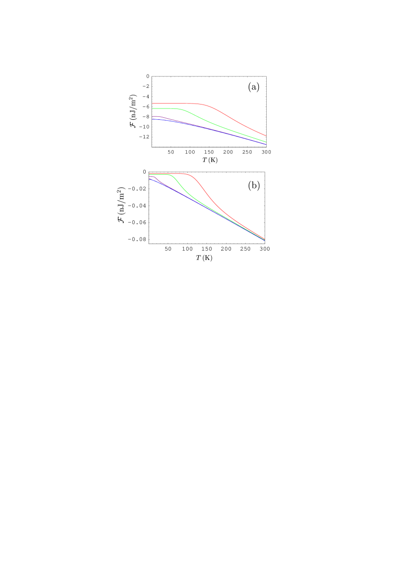
Figure 1: (Color online) The Casimir free energy per unit area as a function of temperature for the interaction of graphene described by the Dirac model with Si plate (a) at $a=100\,$nm and (b) at $a=1\,\mu$m. The lines from top to bottom correspond to the mass gap parameter $\Delta=0.1$, 0.05, 0.01, and $\lesssim 0.001\,$eV, respectively.

The computational results for the free energy per unit area are presented in Fig. 1 as functions of temperature, where the lines from top to bottom correspond to $\Delta$ decreasing from 0.1 eV to 0 eV, (a) at the separation $a=100\,$nm and (b) at $a=1\,\mu$m. As can be seen in Fig. 1(a,b), for each mass gap $\Delta\neq 0$ there exists the temperature interval where the free energy remains nearly constant with increasing temperature. The width of these intervals quickly decreases with decreasing $\Delta$. Thus, at $a=100\,$nm and $\Delta=0.1\,$eV the free energy is nearly constant up to $T=120\,$K. At the same separation, but with $\Delta=0.05\,$eV, the same property holds only up to $T=70\,$K. The widths of intervals, where the free energy remains nearly constant with increasing $T$, are also narrowed with the increase of separation [see Fig. 1(b)]. Note that computations performed for $\Delta\lesssim 0.001\,$eV lead to nearly the same numerical results as for $\Delta=0$ [the lowest lines in Fig. 1(a,b)].

Figure 1 suggests that within the temperature interval, where the free energy is nearly flat, the thermal correction to the Casimir energy at zero temperature should be relatively small. We confirm this conclusion by the direct computation of the thermal correction to the Casimir energy defined as

$$\Delta_{T}{\cal F}(a,T)={\cal F}(a,T)-{\cal F}(a,0)$$ (10)

for the same values of parameters, as in Fig. 1.

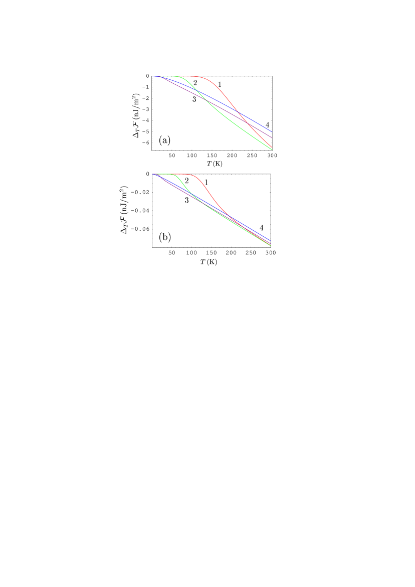
Figure 2: (Color online) The thermal correction to the Casimir energy per unit area at zero temperature as a function of temperature for the interaction of graphene described by the Dirac model with Si plate (a) at $a=100\,$nm and (b) at $a=1\,\mu$m. The lines labeled 1, 2, 3, and 4 correspond to the mass gap parameter $\Delta=0.1$, 0.05, 0.01, and $\lesssim 0.001\,$eV, respectively.

The computational results for the thermal correction as a function of temperature are presented in Fig. 2 at separations (a) $a=100\,$nm and (b) $a=1\,\mu$m. The lines labeled 1, 2, 3, and 4 correspond to the values of mass gap parameter $\Delta=0.1$, 0.05, 0.01, and $\lesssim 0.001\,$eV, respectively. As expected, for each line with $\Delta\neq 0$ there is some interval where the thermal correction remains nearly zero. These intervals are just the same where the Casimir free energy in Fig. 1 remains nearly flat. It is interesting to note that the thermal corrections are monotonously decreasing functions of temperature and have the same negative sign as the free energy. This contrasts with the Drude model approach to the Casimir force between real metals where the thermal correction over a wide temperature interval is positive making the free energy the nonmonotonous function of temperature.23 ; 27

It is instructive also to compute the relative thermal correction to the Casimir energy defined as

$$\delta_{T}{\cal F}(a,T)=\frac{\Delta_{T}{\cal F}(a,T)}{{\cal F}(a,0)}.$$ (11)

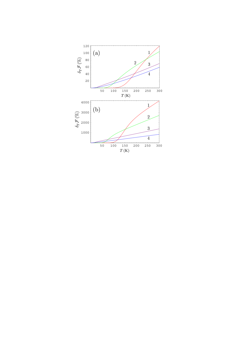
Figure 3: (Color online) The relative thermal correction to the Casimir energy at zero temperature as a function of temperature for the interaction of graphene described by the Dirac model with Si plate (a) at $a=100\,$nm and (b) at $a=1\,\mu$m. The lines labeled 1, 2, 3, and 4 correspond to the mass gap parameter $\Delta=0.1$, 0.05, 0.01, and $\lesssim 0.001\,$eV, respectively.

The computational results are presented in Fig. 3 in percent as functions of temperature at separations distances (a) $a=100\,$nm and (b) $a=1\,\mu$m. The lines 1, 2, 3, and 4 are labeled in the same way as in Fig. 2. As can be seen in Fig. 3, all the relative thermal corrections are monotonously increasing functions of temperature whose character depends crucially on the magnitude of a mass gap parameter $\Delta$. For example, at $a=100\,$nm [Fig. 3(a)] the relative thermal correction of line 1 ($\Delta=0.1\,$eV) is nearly equal to zero below $T=120\,$K but achieves 120.44% at $T=300\,$K. To compare, at the same separation the relative thermal correction of line 4 ($\Delta\lesssim 0.001\,$eV), which is much larger than the corrections of lines 1–3 at low temperatures, achieves only 59.40% at $T=300\,$K. It is seen that at room temperature the relative thermal correction in the Casimir interaction of graphene with Si is rather large even at relatively short separations. From Fig. 3(b) it follows that at $a=1\,\mu$m the relative thermal correction at room temperature exceeds 4000%, i.e., the absolute thermal correction exceeds the Casimir energy at zero temperature by a factor of 40. This makes graphene interesting for experimental investigation of thermal effects in the Casimir force.

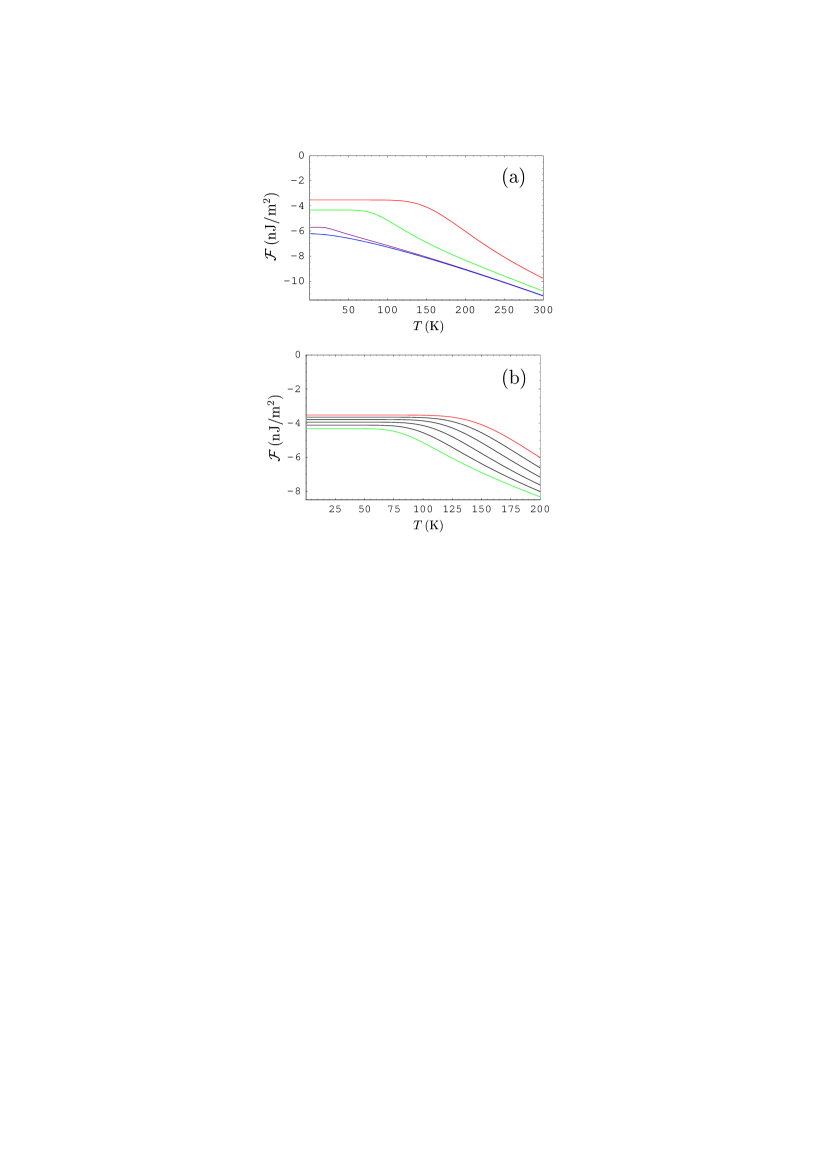
Figure 4: (Color online) The Casimir free energy per unit area as a function of temperature at $a=100\,$nm for the interaction of graphene described by the Dirac model with sapphire plate. The lines from top to bottom correspond to the mass gap parameter (a) $\Delta=0.1$, 0.05, 0.01, and $\lesssim 0.001\,$eV and (b) $\Delta=0.1$, 0.09, 0.08, 0.07, 0.06, and 0.05 eV, respectively.

Next we consider the interaction of graphene described by the Dirac model with sapphire plate. The dielectric permittivity of sapphire along the imaginary frequency axis is well described33 in the Ninham-Parsegian approximation and was already used31 in computations of the Casimir force. Computations of the free energy as a function of temperature were performed in the same way as for silicon. The computational results for $a=100\,$nm are presented in Fig. 4(a) by the four lines from top to bottom for $\Delta=0.1$, 0.05, 0.01, and $\lesssim 0.001\,$eV, respectively. Similar to Fig. 1(a), there are temperature intervals where the free energy remains nearly constant. For sapphire, however, the respective magnitudes of the free energy are smaller than for a silicon. Skipping the computational results at $a=1\,\mu$m [which are similar to those presented in Fig. 1(b)], we present in Fig. 4(b) the more detailed computational results for the free energy in the temperature interval from 0 K to 200 K, where the lines from top to bottom correspond to $\Delta=0.1$, 0.09, 0.08, 0.07, 0.06, and 0.05 eV, respectively. Keeping in mind that the exact value of $\Delta$ is not known, computations of this kind can be useful for the determination of $\Delta$ from the comparison between experiment and theory. For sapphire, the computational results for the absolute and relative thermal corrections are similar to those for silicon (see Figs. 2 and 3). Because of this we do not present them here.

III.2 Free energy as a function of separation

Here, we present the computational results for the interaction of graphene described by the Dirac model with dielectric plates as a function of separation. The same equations and dielectric functions, as in Sec. IIIA, are used. Taking into account that the Casimir free energy strongly depends on separation, we normalize the results obtained on the Casimir energy per unit area between two parallel plates made of ideal metal

$$E_{C}(a)=-\frac{\pi^{2}}{720}\,\frac{\hbar c}{a^{3}}.$$ (12)

In Fig. 5(a) the quantity ${\cal F}/E_{C}$ at $T=77\,$K is plotted as a function of separation over the region from 50 nm to $5\,\mu$m. The lines from bottom to top correspond to the mass gap parameter equal to 0.1, 0.05, and $\lesssim 0.01\,$eV, respectively. In all cases the magnitude of the free energy decreases monotonously with the increase of separation (the increase of ${\cal F}/E_{C}$ is Fig. 5 is explained by the fact that $|E_{C}|$ decreases with separation faster than $|{\cal F}|$). In Fig. 5(b) similar results are shown at $T=300\,$K. Here, to avoid an overlap of the lines, we consider a more narrow separation region from 50 nm to $1\,\mu$m. The bottom and top lines correspond to $\Delta=0.1$ and $\lesssim 0.01\,$eV, respectively. As can be seen from Fig. 5(b), at $T=300\,$K the dependence of the Casimir free energy on the mass gap parameter of the Dirac model is very weak. Moreover, at separations above 50 nm the magnitude of the free energy ${\cal F}$ decreases with separation as $a^{-2}$, so that the quantity ${\cal F}/E_{C}$ is nearly linear function of separation.

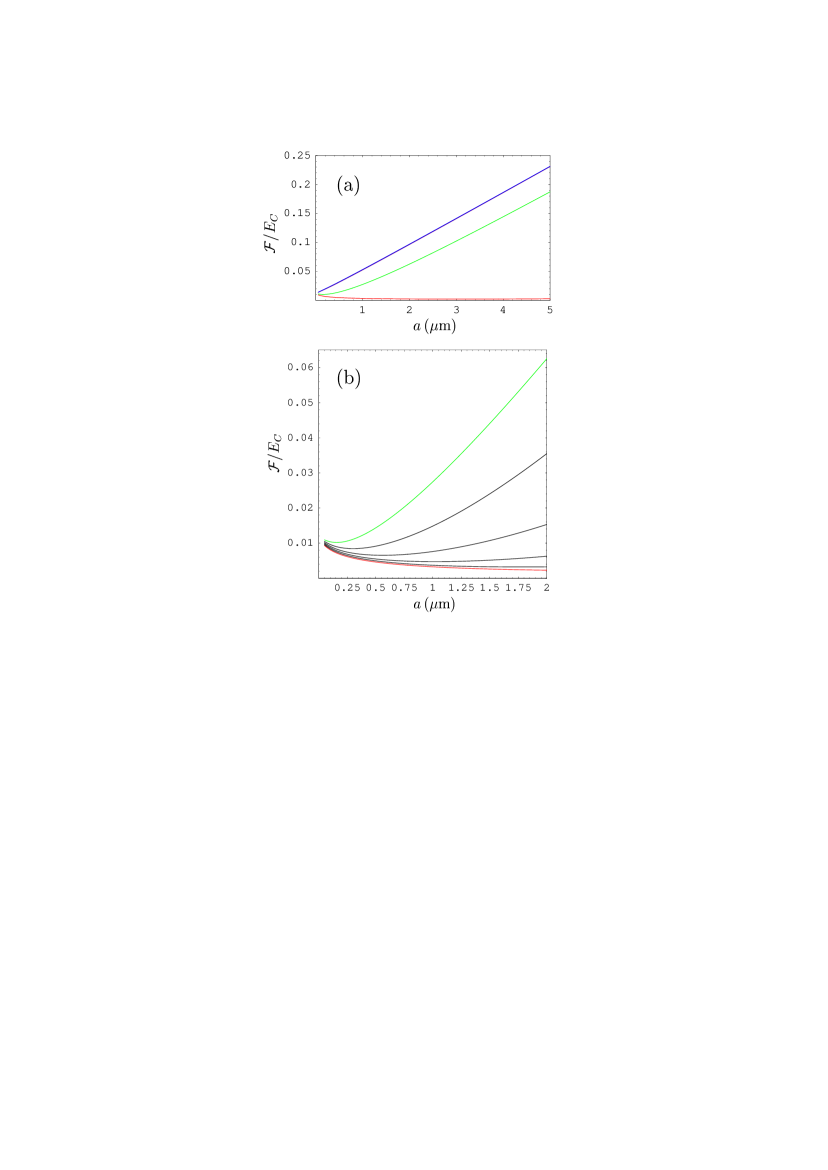
Figure 6: (Color online) The Casimir free energy as a function of separation for the interaction of graphene described by the Dirac model with sapphire plate at $T=77\,$K normalized on the Casimir energy between two parallel ideal metal planes. The lines from bottom to top correspond to the mass gap parameter (a) $\Delta=0.1$, 0.05, $\lesssim 0.01\,$eV and (b) $\Delta=0.1$, 0.09, 0.08, 0.07, 0.06, $0.05\,$eV, respectively.

Similar computations were performed for a graphene interacting with a sapphire plate. In Fig. 6(a) the computational results for ${\cal F}/E_{C}$ as a function of separation at $T=77\,$K are presented, where the lines from bottom to top correspond to $\Delta=0.1$, 0.05, and $\lesssim 0.01\,$eV, respectively. These results are similar to those presented in Fig. 5(a) for a silicon plate. Again, at $T=77\,$K the Casimir free energy is strongly affected by the value of $\Delta$. To illustrate this in more detail, in Fig. 6(b) we plot ${\cal F}/E_{C}$ over the separation region from 50 nm to $2\,\mu$m where the lines from bottom to top correspond to $\Delta=0.1$, 0.09, 0.08, 0.07, 0.06, and 0.05 eV. At $T=300\,$K, similar to Fig. 5(b), the dependence of the free energy on $\Delta$ becomes very weak and one obtains ${\cal F}/E_{C}$ increasing nearly linear with the increase of $a$.

III.3 Asymptotic behavior at high temperature

The asymptotic behavior of the Casimir free energy at high temperature (or, equivalently, at large separations) can be obtained by considering the zero-frequency contribution to the Lifshitz formula (1). This corresponds to large values of the dimensionless parameter $\tau$ introduced after Eq. (4). By putting $l=0$, $\zeta_{0}=0$ in Eq. (4) one arrives at

$$\tilde{\Pi}_{00}(0,y)=8\alpha y^{2}\int_{0}^{1}dx\frac{x(1-x)}{\theta}+\frac{8\alpha}{\tilde{v}_{F}^{2}}\int_{0}^{1}dx$$ (13)

$$~{}\times\left[\frac{\tau}{2\pi}\ln\left(1+2e^{-\frac{2\pi}{\tau}\theta}+e^{-\frac{4\pi}{\tau}\theta}\right)+\frac{\tilde{\Delta}^{2}}{\theta}\frac{1+e^{-\frac{2\pi}{\tau}\theta}}{1+\cosh\frac{2\pi}{\tau}\theta}\right],$$

where

$$\theta\equiv\theta(x,y)=\left[\tilde{\Delta}^{2}+x(1-x)\tilde{v}_{F}^{2}y^{2}\right]^{1/2}.$$ (14)

Equation (13) can be identically rearranged to the form

$$\tilde{\Pi}_{00}(0,y)=\frac{8\alpha}{\tilde{v}_{F}^{2}}\left[\frac{\tau}{\pi}\int_{0}^{1}dx\ln\left(2\cosh\frac{\pi\theta}{\tau}\right)\right.$$

$$~{}~{}~{}~{}~{}~{}~{}~{}~{}~{}\left.-\tilde{\Delta}^{2}\int_{0}^{1}\frac{dx}{\theta}\tanh\frac{\pi\theta}{\tau}\right].$$ (15)

In the limit of high temperature we assume that $\pi\tilde{f}_{F}/\tau\ll 1$. In this case

$$\frac{\pi\theta}{\tau}\approx\frac{\pi\tilde{\Delta}}{\tau}=\frac{\Delta}{2k_{B}T}$$ (16)

and Eq. (15) is reduced to

$$\tilde{\Pi}_{00}(0,y)\approx\frac{8\alpha}{\tilde{v}_{F}^{2}}\,\frac{\tau}{\pi}\,\ln\left(2\cosh\frac{\pi\tilde{\Delta}}{\tau}\right)\equiv\tilde{\Pi}_{00}(0).$$ (17)

From Eq. (2) the TM reflection coefficient on graphene at zero Matsubara frequency is given by

$$r_{\rm TM}^{(g)}(0,y) = \frac{\tilde{\Pi}_{00}(0,y)}{\tilde{\Pi}_{00}(0,y)+2y}=1-\frac{2y}{\tilde{\Pi}_{00}(0,y)+2y}$$ (18)

$$\approx 1-\frac{2y}{\tilde{\Pi}_{00}(0)}.$$

Taking into account that in accordance with Eq. (9) for dielectric materials $r_{\rm TE}^{(p)}(0,y)=0$, we obtain from Eqs. (1) and (18) the following asymptotic expression for the Casimir free energy at large $\tau$:

$${\cal F}(a,T)\approx\frac{k_{B}T}{16\pi a^{2}}\int_{0}^{\infty}\!\!\!\!\!ydy\ln\left\{1-r_{0}\left[1-\frac{2y}{\tilde{\Pi}_{00}(0)}\right]e^{-y}\right\},$$ (19)

where the TM reflection coefficient of the dielectric plate at zero Matsubara frequency

$$r_{\rm TE}^{(p)}(0,y)\equiv r_{0}=\frac{\varepsilon(0)-1}{\varepsilon(0)+1}.$$ (20)

Equation (20) can be rearranged to the form

$${\cal F}(a,T)\approx\frac{k_{B}T}{16\pi a^{2}}\int_{0}^{\infty}\!\!\!ydy\ln\left\{\vphantom{\left[\frac{2}{\tilde{\Pi}_{00}}\frac{r_{0}e^{-y}}{r_{0}e^{-y}}\right]}(1-r_{0}e^{-y})\right.$$

$$~{}~{}~{}\times\left.\left[1+\frac{2y}{\tilde{\Pi}_{00}(0)}\frac{r_{0}e^{-y}}{1-r_{0}e^{-y}}\right]\right\}.$$ (21)

In view of the fact that $\tau/(\pi\tilde{v}_{F})\gg 1$, one obtains

$${\cal F}(a,T)\approx\frac{k_{B}T}{16\pi a^{2}}\int_{0}^{\infty}\!\!\!\!\!ydy\left[\ln(1-r_{0}e^{-y})+\frac{2y}{\tilde{\Pi}_{00}(0)}\frac{r_{0}e^{-y}}{1-r_{0}e^{-y}}\right].$$ (22)

Performing the integration in Eq. (22) we arrive at the following asymptotic expression for the Casimir free energy:

$${\cal F}(a,T)=\frac{k_{B}T}{16\pi a^{2}}\left[-{\rm Li}_{3}(r_{0})+\frac{4}{\tilde{\Pi}_{00}(0)}{\rm Li}_{3}(r_{0})\right]$$ (23)

$$~{}~{}~{}~{}=-\frac{k_{B}T}{16\pi a^{2}}{\rm Li}_{3}(r_{0})\left[1-\frac{\pi\tilde{v}_{F}^{2}}{2\alpha\tau\ln\left(2\cosh\frac{\pi\tilde{\Delta}}{\tau}\right)}\right],$$

where ${\rm Li}_{n}(z)$ is the polylogarithm function.

The application region of Eq. (23) depends on the specific values of parameters. Thus, for Si at $T=300\,$K Eq. (23) leads to less than 1% errors in the values of the free energy, as compared with the results of numerical computations, at $a\geq 500\,$nm for graphene with $\Delta=0.1\,$eV and at $a\geq 1\,\mu$m for graphene with $\Delta=0.01\,$eV. For Si at $T=77\,$K and graphene with $\Delta=0.1\,$eV Eq. (23) is not yet applicable at $a=5\,\mu$m and for graphene with $\Delta=0.01\,$eV works well for $a\geq 4\,\mu$m.

It is interesting to compare the asymptotic expression (23) with other results obtained in the literature. Thus, using the nonlocal dielectric function in the random phase approximation, the free energy of graphene interacting with a dielectric substrate (SiO₂) at large separations was found21b to decrease as $a^{-3}$. This is not in accordance with the main term of our result (23) which demonstrates the classical limit, as is expected at large $a$. Note that another work34a models the dielectric properties of graphene by the Drude-type function and arrives at the $a^{-2}$ scaling for graphene-graphene interaction which satisfies the classical limit.

IV Thermal interaction of graphene described by the Dirac model with metallic plate

The case of graphene interacting with metallic plate is of special interest. As was mentioned in Sec. I, there are two different theoretical approaches to the description of Casimir effect between real-metal plates. The Drude model approach takes into account the relaxation properties of conduction electrons. In the framework of this approach, the imaginary part of the dielectric permittivity of the Drude model is used to extrapolate ${\rm Im}\,\varepsilon^{\rm opt}(\omega)$, obtained from the measured optical data, to zero frequency. By contrast, the plasma model approach disregards relaxation processes and extrapolates $\varepsilon^{\rm opt}(\omega)$ to zero frequency by means of the simple plasma model. Although the Drude model approach may seem preferable, as it takes into account some really existing property of metals, the experimental situation more likely favors the plasma model approach. In a series of precise independent measurements performed by the two experimental groups34 ; 35 ; 36 ; 37 ; 38 the Drude model approach was excluded at a high confidence level (several experiments39 ; 40 ; 41 ; 42 ; 43 ; 44 also excluded the influence of free charge carriers, that are present in dielectric materials at room temperature, on the Casimir force). The two experiments that support the Drude model approach45 ; 46 are not independent measurements of the Casimir force; they are based on fitting procedures between measured data for the total force and theoretical predictions using hypothetical models for the electric contribution to it. Here, we show that in the interaction of graphene described by the Dirac model with metallic plate the results obtained are not sensitive to the approach used (either Drude or plasma). This is, however, not the case when graphene is described by the hydrodynamic model (see Sec. V).

IV.1 Free energy as a function of temperature

Numerical computations of the Casimir free energy per unit area between graphene described by the Dirac model and Au plate were performed by using Eqs. (1), (2), (4)–(6) and (9) with $\mu_{l}=1$. The dielectric permittivity of Au along the imaginary frequency axis was described either by the generalized Drude-like model with temperature-dependent relaxation parameter47 ; 48 or by the generalized plasma-like model.23 ; 27 ; 37 These models use the six-oscillator approximation for the optical data extrapolated to zero frequency by means of simple Drude and plasma models, respectively, with the plasma frequency $\omega_{p}=9.0\,$eV and the relaxation parameter at room temperature $\gamma=0.035\,$eV. At lower $T$ the lower values of $\gamma$ according to the standard theory of electron-phonon interaction have been used.49

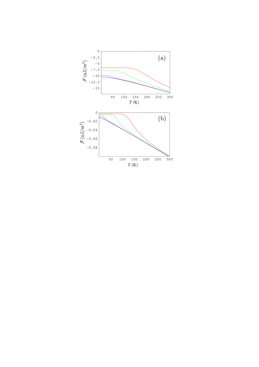
Figure 7: (Color online) The Casimir free energy per unit area as a function of temperature for the interaction of graphene described by the Dirac model with Au plate (a) at $a=100\,$nm and (b) at $a=1\,\mu$m. The lines from top to bottom correspond to the mass gap parameter $\Delta=0.1$, 0.05, 0.01, and $\lesssim 0.001\,$eV, respectively.

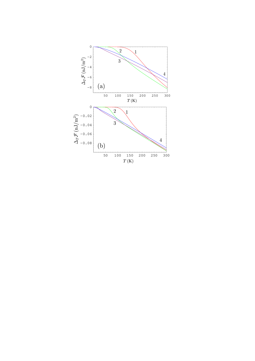
Figure 8: (Color online) The thermal correction to the Casimir energy per unit area at zero temperature as a function of temperature for the interaction of graphene described by the Dirac model with Au plate (a) at $a=100\,$nm and (b) at $a=1\,\mu$m. The lines labeled 1, 2, 3, and 4 correspond to the mass gap parameter $\Delta=0.1$, 0.05, 0.01, and $\lesssim 0.001\,$eV, respectively.

The computational results using the Drude- and plasma-model approaches are found to be indistinguishable. Thus, at $T=77\,$K the relative difference between the Casimir free energies computed using both approaches achieves the maximum value of 0.02% at $a=50\,$nm, does not depend on $\Delta$ in the limits of our computational accuracy, and decreases with the increase of separation. At $T=300\,$K this difference achieves the maximum values of 0.06% at $\Delta=0$ and 0.07% at $\Delta=0.1\,$eV, and again decreases with increasing $a$. Figure 7 presents the Casimir free energy per unit area as a function of temperature (a) for $a=100\,$nm and (b) for $a=1\,\mu$m. It can be seen that Fig. 7 demonstrates the same characteristic features, as Figs. 1 and 4 plotted for dielectric plates, but the magnitudes of the free energy for the case of metallic plate are larger. The most important novel qualitative effect, which is found for both dielectrics and metals, is that for each nonzero $\Delta$ the free energy is nearly unchanged with the increase of $T$ within some temperature interval. In Fig. 8 we present the computational results for the absolute thermal correction to the Casimir energy at zero temperature, defined in Eq. (10), as a function of temperature. The lines 1, 2, 3, and 4 correspond to the values of the mass gap parameter $\Delta=0.1$, 0.05, 0.01, and $\lesssim 0.001\,$eV, respectively. This figure is analogous to Fig. 2 plotted for Si. It demonstrates that for a metallic plate the thermal correction in the graphene-plate geometry behaves qualitatively in the same way as for a dielectric plate, but with slightly larger magnitudes of the thermal correction.

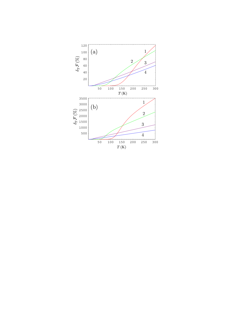
Figure 9: (Color online) The relative thermal correction to the Casimir energy at zero temperature as a function of temperature for the interaction of graphene described by the Dirac model with Au plate (a) at $a=100\,$nm and (b) at $a=1\,\mu$m. The lines labeled 1, 2, 3, and 4 correspond to the mass gap parameter $\Delta=0.1$, 0.05, 0.01, and $\lesssim 0.001\,$eV, respectively.

The computational results for the relative thermal correction, defined in Eq. (11) are presented in Fig. 9 as a function of temperature. The lines 1, 2, 3, and 4 again correspond to the same respective $\Delta$, as in Fig. 8. Figure 9 is analogous to Fig. 3 plotted for a dielectric plate (silicon). For a metallic plate at $a=100\,$nm the relative thermal correction at room temperature appears only slightly larger than for a dielectric plate. At $a=1\,\mu$m at room temperature the relative thermal correction for Au is smaller than for Si. This is explained by different values of the Casimir energy at zero temperature.

IV.2 Free energy as a function of separation

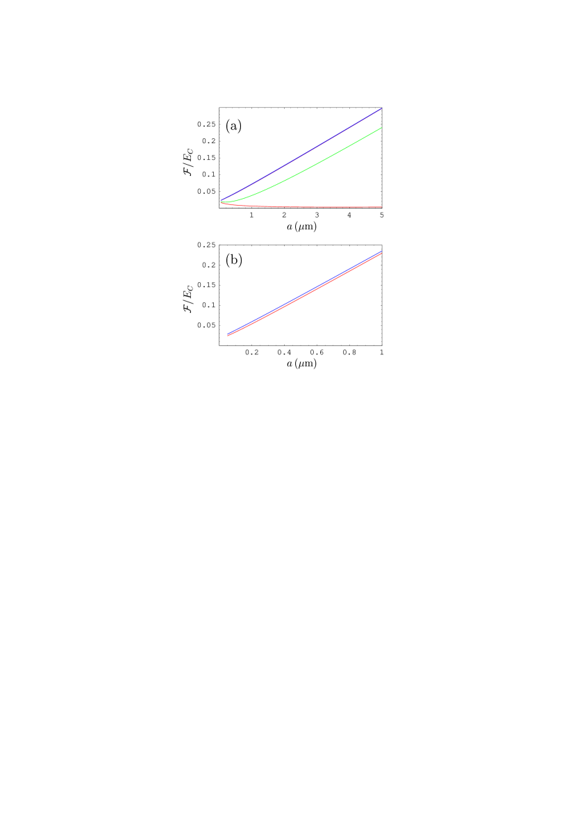
Figure 10: (Color online) The Casimir free energy as a function of separation for the interaction of graphene described by the Dirac model with Au plate (a) at $T=77\,$K and (b) at $T=300\,$K normalized on the Casimir energy between two parallel ideal metal planes. The lines from bottom to top correspond to the mass gap parameter (a) $\Delta=0.1$, 0.05, $\lesssim 0.01\,$eV and (b) $\Delta=0.1$, $\lesssim 0.01\,$eV, respectively.

Keeping in mind that in most experiments on the Casimir force the temperature is preserved constant and measurements are performed at different separation distances, here we present the computational results for a free energy of graphene-metal interaction as a function of separation. In Fig. 10(a) the free energy of graphene interacting with Au plate normalized on the Casimir energy between ideal metal planes (12) is shown. The three lines from bottom to top correspond to the values of mass gap parameter $\Delta=0.1$, 0.05, and $\lesssim 0.01\,$eV, respectively. The obtained values of the free energy are larger than for graphene interacting with Si plate [compare with Fig. 5(a)]. At $T=300\,$K the dependence of the computational results on the mass gap parameter becomes not so pronounced as in Fig. 10(a). This can be seen in Fig. 10(b) where the bottom and top lines correspond to $\Delta=0.1\,$eV and $\lesssim 0.01\,$eV, respectively.

It is interesting to consider the Casimir interaction of graphene with a ferromagnetic metal. It was shown50 ; 51 that at room temperature the ferromagnetic properties of real metals may influence the Casimir force only through the contribution of the zero-frequency term of the Lifshitz formula. Recently the gradient of the Casimir force between a nonmagnetic Au sphere and a magnetic metal (Ni) plate has been measured.52 We have computed the Casimir free energy per unit area between a graphene described by the Dirac model and Ni plate using the same formalism, as for an Au plate. The dielectric permittivity of Ni along the imaginary frequency axis was found from the tabulated optical data53 extrapolated to zero frequency either by the Drude or by the plasma model with the plasma frequency $\omega_{p}=4.89\,$eV and the relaxation parameter at room temperature $\gamma=0.0436\,$eV.53 ; 54 The value of $\mu(0)=110$ for the static magnetic permeability of Ni has been used. It was found that relative differences in the computational results for the free energy of graphene-Ni interaction, when Ni is described using the Drude- and plasma-model approaches, are as small as computed above for the interaction of graphene with an Au plate. The influence of magnetic properties on the free energy was also shown to be negligibly small. The relative difference between the free energies of graphene-Ni and graphene-Au interactions for graphene with $\Delta=0.1\,$eV computed at $T=300\,$K is equal to 6% at $a=100\,$nm and decreases to 1% at $a=1\,\mu$m. It is less for smaller values of the mass gap parameter. Note that even these small differences are not due to magnetic properties of Ni but due to different plasma frequency and optical properties of Ni as compared to Au.

IV.3 Asymptotic behavior at high temperature

Now we derive the analytic expression for the Casimir free energy of graphene described by the Dirac model interacting with metallic plate at $\tau\gg 1$. The contribution of the TM reflection coefficient for graphene interacting with dielectric plate was obtained in Eq. (22). Taking into account that for metallic materials $r_{0}$ defined in Eq. (20) is equal to unity, one obtains from Eq. (22)

$${\cal F}_{\rm TM}(a,T)\approx\frac{k_{B}T}{16\pi a^{2}}\int_{0}^{\infty}\!\!\!\!ydy\left[\ln(1-e^{-y})+\frac{2y}{\tilde{\Pi}_{00}(0)}\frac{e^{-y}}{1-e^{-y}}\right].$$ (24)

Calculating the integral with respect to $y$ and using Eq. (17), we arrive at

$${\cal F}_{\rm TM}(a,T)=-\frac{k_{B}T}{16\pi a^{2}}\zeta(3)\left[1-\frac{4}{\tilde{\Pi}_{00}(0)}\right]$$ (25)

$$~{}~{}\approx-\frac{k_{B}T}{16\pi a^{2}}\zeta(3)\left[1-\frac{\pi\tilde{v}_{F}^{2}}{2\alpha\tau\ln\left(2\cosh\frac{\pi\tilde{\Delta}}{\tau}\right)}\right],$$

where $\zeta(z)$ is the Riemann zeta function. This result in the special case $\tilde{\Delta}=0$ was obtained in Ref. 55 . Note that for a dielectric plate considered in Sec. IIIC the contribution of the TM mode was in fact equal to the total free energy because $r_{\rm TE}^{(p)}(0,y)=0$ for dielectrics. For metals this is in general not so (see below).

The TE reflection coefficient for graphene at zero Matsubara frequency is obtained from Eq. (2)

$$r_{\rm TE}^{(g)}(0,y)=-\frac{\tilde{\Pi}_{tr}(0,y)-\tilde{\Pi}_{00}(0,y)}{\tilde{\Pi}_{tr}(0,y)-\tilde{\Pi}_{00}(0,y)+2y}.$$ (26)

From Eq. (6) taken at $l=0$, $\zeta_{0}=0$ and Eq. (13) it is easily seen that

$$\tilde{\Pi}_{tr}(0,y)-\tilde{\Pi}_{00}(0,y)=8\alpha\tilde{v}_{F}^{2}y^{2}\int_{0}^{1}dx\frac{x(1-x)}{\theta}$$

$$~{}~{}~{}~{}~{}~{}~{}\times\left(1-\frac{1+e^{-\frac{2\pi}{\tau}\theta}}{1+\cosh\frac{2\pi}{\tau}\theta}\right),$$ (27)

where the quantity $\theta$ is defined in Eq. (14). After identical transformations with account of Eq. (16) the result is

$$\tilde{\Pi}_{tr}(0,y)-\tilde{\Pi}_{00}(0,y)=8\alpha\tilde{v}_{F}^{2}y^{2}\int_{0}^{1}dx\frac{x(1-x)}{\theta}\tanh\frac{\pi\theta}{\tau}$$

$$~{}~{}~{}~{}~{}\approx\frac{8\alpha\tilde{v}_{F}^{2}y^{2}}{\tilde{\Delta}}\tanh\frac{\pi\tilde{\Delta}}{\tau}\int_{0}^{1}x(1-x)dx$$

$$~{}~{}~{}~{}~{}=\frac{4\alpha\tilde{v}_{F}^{2}y^{2}}{3\tilde{\Delta}}\tanh\frac{\pi\tilde{\Delta}}{\tau}.$$ (28)

This quantity is negligibly small as compared to unity because the main contribution to the Lifshitz formula (1) is given by $y\sim 1$ and for $\tilde{\Delta}\to 0$ one has

$$\tilde{\Pi}_{tr}(0,y)-\tilde{\Pi}_{00}(0,y)\to\frac{4\pi\alpha\tilde{v}_{F}^{2}y^{2}}{3\tau}.$$ (29)

Thus, we can neglect by the difference of polarization operators in the denominator of Eq. (26) and get

$$r_{\rm TE}^{(g)}(0,y)\approx-\frac{2\alpha\tilde{v}_{F}^{2}y}{3\tilde{\Delta}}\tanh\frac{\pi\tilde{\Delta}}{\tau}.$$ (30)

Using the Lifshitz formula (1) and Eq. (30) for the contribution of the TE reflection coefficient to the Casimir free energy of graphene-metal interaction at high temperature, we arrive at

$${\cal F}_{\rm TE}(a,T)\approx\frac{k_{B}T}{16\pi a^{2}}\int_{0}^{\infty}\!\!\!\!\!ydy\ln\left[1-r_{\rm TE}^{(g)}(0,y)r_{\rm TE}^{(p)}(0,y)e^{-y}\right]$$

$$~{}~{}~{}\approx\frac{k_{B}T}{24\pi a^{2}}\,\frac{\alpha\tilde{v}_{F}^{2}}{\tilde{\Delta}}\tanh\frac{\pi\tilde{\Delta}}{\tau}\int_{0}^{\infty}\!\!\!y^{2}dy\,r_{\rm TE}^{(p)}(0,y)e^{-y}.$$ (31)

Here we have used that $|r_{\rm TE}^{(g)}(0,y)|\ll 1$ at $y\sim 1$.

Now we are in a position to consider metallic plates made of nonmagnetic and magnetic metals described within both the Drude and the plasma model approaches and in all cases find the high-temperature behavior of the total Casimir free energy. We begin with a nonmagnetic metal described by the Drude model approach. In this case from Eq. (9) one obtains that $r_{\rm TE}^{(p)}(0,y)=0$ and in accordance with Eq. (31) the TE contribution to the free energy ${\cal F}_{\rm TE}(a,T)$ vanishes. Thus, for the plate made of a nonmagnetic Drude metal the total free energy of graphene-metal interaction at high temperature is given by Eq. (25).

Next we consider a nonmagnetic metal described by the plasma-model approach. In this case from Eq. (9) we have

$$r_{\rm TE}^{(p)}(0,y)=\frac{\delta y-\sqrt{1+\delta^{2}y^{2}}}{\delta y+\sqrt{1+\delta^{2}y^{2}}}\approx-(1-2\delta y+2\delta^{2}y^{2}),$$ (32)

where the parameter $\delta$ is defined as

$$\delta\equiv\frac{\omega_{c}}{\omega_{p}}=\frac{c}{2a\omega_{p}}=\frac{\delta_{p}}{2a}\ll 1$$ (33)

and $\delta_{p}\equiv c/\omega_{p}$ is the effective penetration depth of electromagnetic oscillations into the metal. Substituting Eq. (32) in Eq. (31) and integrating with respect to $y$, one obtains

$${\cal F}_{\rm TE}(a,T)\approx-\frac{k_{B}T}{12\pi a^{2}}\,\frac{\alpha\tilde{v}_{F}^{2}}{\tilde{\Delta}}\tanh\frac{\pi\tilde{\Delta}}{\tau}(1-6\delta+24\delta^{2}).$$ (34)

The total asymptotic expression for the free energy at high temperature is given by the sum of (25) and (34). Note that the contribution of the TE mode (34) is a negligibly small correction because $\alpha\tilde{v}_{F}^{2}\sim 10^{-7}$.

We are coming now to the consideration of magnetic metals described by the Drude model. From Eq. (9) it follows

$$r_{\rm TE}^{(p)}(0,y)=\frac{\mu(0)-1}{\mu(0)+1}.$$ (35)

The substitution of this reflection coefficient in Eq. (31) results in

$${\cal F}_{\rm TE}(a,T)\approx\frac{k_{B}T}{24\pi a^{2}}\,\frac{\alpha\tilde{v}_{F}^{2}}{\tilde{\Delta}}\,\tanh\frac{\pi\tilde{\Delta}}{\tau}\,\,\frac{\mu(0)-1}{\mu(0)+1}\int_{0}^{\infty}\!\!\!y^{2}e^{-y}dy$$

$$~{}~{}~{}~{}~{}~{}~{}~{}=\frac{k_{B}T}{12\pi a^{2}}\,\frac{\alpha\tilde{v}_{F}^{2}}{\tilde{\Delta}}\tanh\frac{\pi\tilde{\Delta}}{\tau}\,\,\frac{\mu(0)-1}{\mu(0)+1}.$$ (36)

This term is again negligibly small, as compared to ${\cal F}_{\rm TM}(a,T)$, so that the total Casimir free energy at high temperature is well described by Eq. (25).

Finally we consider the asymptotic expression for the free energy of graphene interacting with a magnetic metal described by the plasma model. In this case from Eq. (9) we get

$$r_{\rm TE}^{(p)}(0,y)=\frac{\delta\sqrt{\mu(0)}y-\sqrt{1+\frac{\delta^{2}y^{2}}{\mu(0)}}}{\delta\sqrt{\mu(0)}y+\sqrt{1+\frac{\delta^{2}y^{2}}{\mu(0)}}}$$ (37)

$$~{}~{}~{}~{}~{}~{}~{}~{}~{}\approx-\left[1-2\delta\sqrt{\mu(0)}y+2\delta^{2}\mu(0)y^{2}\right].$$

This is similar to Eq. (32) with the replacement of $\delta$ for $\delta\sqrt{\mu(0)}$. Thus, instead of Eq. (34), one obtains

$${\cal F}_{\rm TE}(a,T)\approx-\frac{k_{B}T}{12\pi a^{2}}\,\frac{\alpha\tilde{v}_{F}^{2}}{\tilde{\Delta}}\tanh\frac{\pi\tilde{\Delta}}{\tau}$$

$$~{}~{}~{}~{}~{}~{}~{}~{}~{}~{}\times\left[1-6\delta\sqrt{\mu(0)}+24\delta^{2}\mu(0)\right].$$ (38)

The total asymptotic expression for the free energy at high temperature is given by the sum of Eq. (25) and negligibly small addition (38) depending on the properties of magnetic metal. The obtained analytic expressions were found in good agreement with the results of numerical computations within appropriate temperature (separation) intervals.

V Comparison between hydrodynamic and Dirac models of graphene

On this section we compare the computational results for the free energy of graphene-plate interaction obtained using two different models of graphene discussed in Secs. I and II. We find separation regions where the predictions of both models are distinct and similar and compare respective asymptotic expressions for the free energy at high temperature (large separations).

V.1 Comparison between computational results for graphene described by two different models

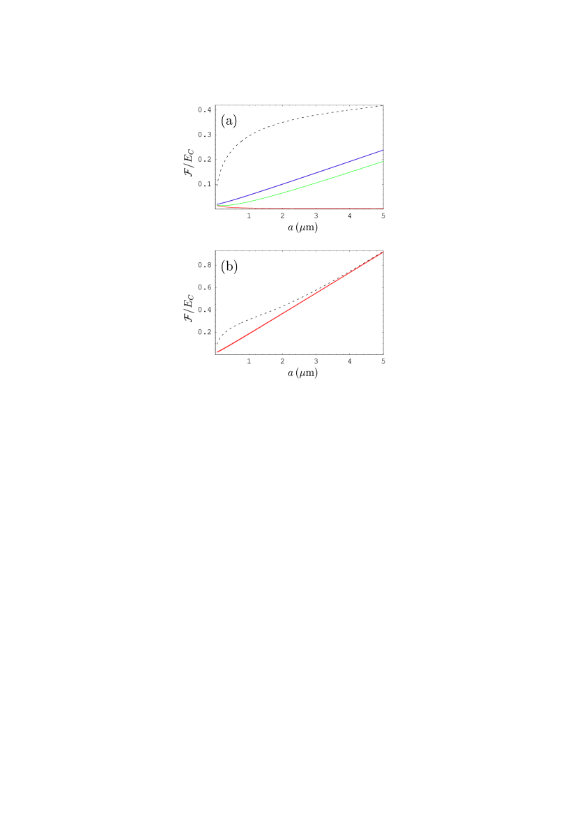
Figure 11: (Color online) The Casimir free energy as a function of separation for the interaction of graphene described by the hydrodynamic model (dashed lines) and by the Dirac model (solid lines) with Si plate (a) at $T=77\,$K and (b) at $T=300\,$K normalized on the Casimir energy between two parallel ideal metal planes. The solid lines correspond (a) from bottom to top to the mass gap parameter $\Delta=0.1$, 0.05, $\lesssim 0.01\,$eV, respectively, and (b) to $\Delta=0.1\,$eV.

Keeping in mind the possibility to compare theoretical predictions for the Casimir force with the experimental data, we calculate the free energy of graphene-plate interaction as a function of separation for both dielectric and metallic plates. Computations were performed using the Lifshitz formula (1) where the reflection coefficients (17) for graphene in the framework of the hydrodynamic model were used. The computational results for ${\cal F}/E_{C}$ as a function of separation are presented in Fig. 11 by the dashed lines (a) at $T=77\,$K and (b) at $T=300\,$K. In the same figure the respective results for ${\cal F}/E_{C}$ computed using the Dirac model of graphene are reproduced from Fig. 5(a,b) by the solid lines. The solid lines in Fig. 11(a) from bottom to top correspond to $\Delta=0.1$, 0.05, and $\lesssim 0.01\,$eV, respectively. Note that in the scale used in Fig. 11(b) the two lines of Fig. 5(b) overlap. They are shown as a single solid line in Fig. 11(b).

As is seen in Fig. 11(a), at $T=77\,$K the hydrodynamic model of graphene predicts much larger magnitudes of the Casimir free energy than the Dirac model. Thus, at $T=77\,$K the predictions of the hydrodynamic model for $|{\cal F}|$ at $a=0.5\,\mu$m is by factors of 36.0 and 6.7 larger than predictions of the Dirac model with $\Delta=0.1\,$eV and $\Delta\lesssim 0.01\,$eV, respectively. At $a=1.5\,\mu$m the respective factors are 97.9 and 4.2. At $T=300\,$K [see Fig. 11(b)] the predictions of the hydrodynamic model are larger than the predictions of the Dirac model by the factors of 2.5 and 1.3 at $a=0.5\,\mu$m and $a=1.5\,\mu$m, respectively. As is seen in Fig. 11(b), at $T=300\,$K, $a>4\,\mu$m the asymptotic regime of large $\tau$ is already achieved and the predictions of the hydrodynamic and Dirac models almost coincide. At $T=77\,$K [Fig. 11(a)] the asymptotic regime of large $\tau$ is achieved at much larger separations than those shown in the figure.

Now we compare the predictions of the hydrodynamic and Dirac models of graphene interacting with a metallic plate. All computations were performed using the same formalism as above. We considered the plates made of a nonmagnetic metal Au and a magnetic metal Ni. Each of these metals was described either using the Drude- or the plasma-model approach.

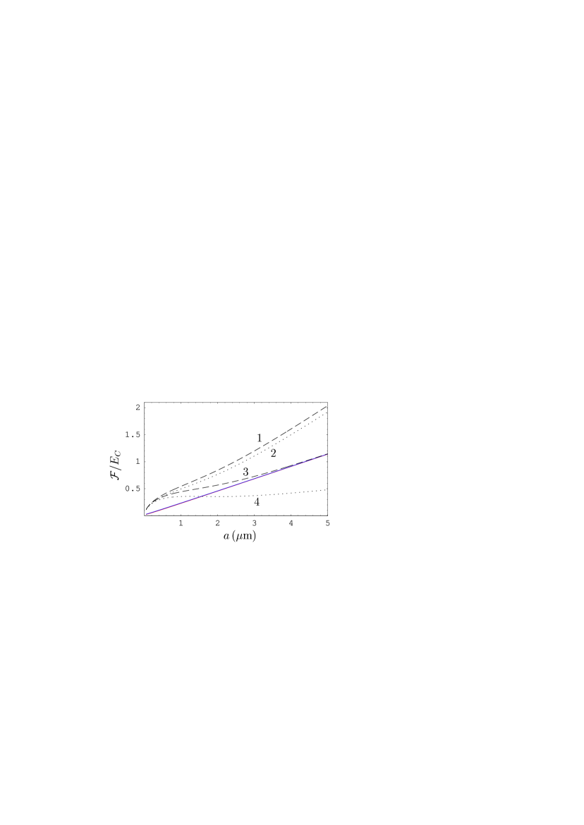
Figure 12: (Color online) The Casimir free energy as a function of separation for the interaction of graphene described by the hydrodynamic model (dashed and dotted lines) and by the Dirac model (solid line) with Au (dashed lines labeled 1 and 3) and Ni (dotted lines labeled 2 and 4) at $T=300\,$K normalized on the Casimir energy between two parallel ideal metal planes. For lines labeled 1 and 2 metal is described by the plasma-model approach, and for lines labeled 3 and 4 by the Drude-model approach.

The computational results for the normalized free energy ${\cal F}/E_{C}$ are presented in Fig. 12 at $T=300\,$K as a function of separation. In this figure, the solid line is reproduced from Fig. 10(b) [note that in the scale of Fig. 12 the two solid lines in Fig. 10(b) overlap]. This line is obtained using the Dirac model of graphene interacting with a metallic plate, be it Au or Ni (see Sec. IVB). The dashed and dotted lines 1, 2, 3, and 4 are obtained from computations using the hydrodynamic model of graphene. The computational data shown by the dashed lines 1 and 3 were found for an Au plate described by the plasma- and Drude-model approaches, respectively. The data shown by the dotted lines 2 and 4 were computed for a Ni plate also described by the respective plasma- and Drude-model approaches. As can be seen in Fig. 12, the free energy of graphene-metal interaction with graphene described by the hydrodynamic model strongly depends on the metal used (magnetic or nonmagnetic) and on the chosen approach to the description of dielectric properties. Only for the nonmagnetic metal (Au) described by the Drude model (line 3) the behavior of the free energy is qualitatively similar to the case of dielectric plate and nears the prediction of the Dirac model at large separations [compare with Fig. 11(b)].

As an example, the Casimir free energy of graphene-metal interaction computed using the hydrodynamic model of graphene at $a=1\,\mu$m, $T=300\,$K is larger than the same quantity computed using the Dirac model by factors of 2.37 (for an Au plate described by the plasma model), 2.15 (for a Ni plate described by the plasma model), 1.93 (for an Au plate described by the Drude model), and 1.55 (for a Ni plate described by the Drude model). This allows comparison between different theoretical predictions and experimental data. It is interesting that for lines 1–3 the magnitude of ${\cal F}$ predicted by the hydrodynamic model is always larger than for the predictions of the Dirac model (solid line). As to the line 4 (Ni described by the Drude model), the prediction for $|{\cal F}|$ from the hydrodynamic model becomes less than from the Dirac model at $a\approx 1.55\,\mu$m and remains so at larger separations. Thus, at $a=5\,\mu$m the ratio between the predictions of hydrodynamic and Dirac models is equal to 0.42.

V.2 Asymptotic behavior at high temperature

As was mentioned in Sec. IIIC, at high temperature (large separations) the zero-frequency term of the Lifshitz formula (1) alone determines the Casimir free energy. The reflection coefficients on the graphene, described by the hydrodynamic model, at zero frequency follow from Eq. (7)

$$r_{\rm TM}^{(g)}(0,y)=1,\qquad r_{\rm TE}^{(g)}(0,y)=-\frac{\tilde{K}}{\tilde{K}+y}.$$ (39)

Taking into account that for a hydrodynamic model at $T=300\,$K the high-temperature regime starts at $a>5\,\mu$m, we find from Eq. (8) that at these separations $\tilde{K}>6.75$. Substituting Eq. (39) for the reflection coefficient $r_{\rm TM}^{(g)}$ into the zero-frequency term of the Lifshitz formula (1), for the TM contribution to the free energy at high temperature one obtains

$${\cal F}_{\rm TM}(a,T)=\frac{k_{B}T}{16\pi a^{2}}\int_{0}^{\infty}\!\!\!\!\!ydy\ln\left[1-r_{\rm TM}^{(p)}(0,y)e^{-y}\right].$$ (40)

For a dielectric plate, using Eq. (20) and integrating in Eq. (40), we get

$${\cal F}_{\rm TM}(a,T)=-\frac{k_{B}T}{16\pi a^{2}}{\rm Li}_{3}(r_{0}).$$ (41)

As noted in Sec. IIIC, for a dielectric plate the contribution of the TE mode to the free energy vanishes. Thus, Eq. (41) provides the complete expression for the free energy of graphene-dielectric interaction at high temperature. Equation (41) coincides with the first term in Eq. (23) obtained for graphene described by the Dirac model [remind that for the Dirac model of graphene the asymptotic expression (23) becomes applicable at much smaller separations at the same room temperature; see Fig. 11(b)].

For a metallic plate, replacing $r_{0}$ with unity, we arrive at

$${\cal F}_{\rm TM}(a,T)=-\frac{k_{B}T}{16\pi a^{2}}\zeta(3).$$ (42)

This result coincides with the first term of the asymptotic expression (25) obtained for graphene described by the Dirac model. Equation (42) provides the total asymptotic expression for the free energy only in the case when a nonmagnetic metal of the plate is described by the Drude model (see the dashed line 3 approaching the solid line in Fig. 12 when the separation distance increases).

Now we consider the contribution of the TE mode to the free energy of graphene-metal Casimir interaction. From Eq. (39) we have

$$r_{\rm TE}^{(g)}(0,y)=-\frac{1}{1+\beta y}\approx-(1-\beta y+\beta^{2}y^{2}),$$ (43)

where $\beta=1/\tilde{K}$ takes the maximum value $\beta_{\max}\approx 0.15$ and decreases with further increase of separation. Then, for the contribution of the TE mode to the free energy at high temperature one obtains

$${\cal F}_{\rm TE}(a,T)\approx\frac{k_{B}T}{16\pi a^{2}}\int_{0}^{\infty}\!\!\!\!\!ydy\ln\left[\vphantom{r_{\rm TE}^{(p)}}1+(1-\beta y+\beta^{2}y^{2})\right.$$

$$~{}~{}~{}~{}~{}~{}~{}~{}~{}~{}~{}~{}~{}~{}~{}~{}~{}~{}~{}~{}\left.\times r_{\rm TE}^{(p)}(0,y)e^{-y}\right].$$ (44)

For a nonmagnetic metal described by the plasma model the reflection coefficient $r_{\rm TE}^{(p)}(0,y)$ is given by Eq. (32). Substituting Eq. (32) in Eq. (44), we find

$${\cal F}_{\rm TE}(a,T)\approx\frac{k_{B}T}{16\pi a^{2}}\left[\int_{0}^{\infty}\!\!\!\!\!ydy\ln(1-e^{-y})+(\beta+2\delta)\int_{0}^{\infty}\!\frac{y^{2}dy}{e^{y}-1}\right.$$

$$~{}~{}\left.-\frac{\beta^{2}}{2}\int_{0}^{\infty}\!\!\!y^{2}dy\frac{2e^{y}-1}{(e^{y}-1)^{2}}-2\delta(\beta+\delta)\int_{0}^{\infty}\!\frac{y^{2}e^{y}dy}{(e^{y}-1)^{2}}\right]$$ (45)

$$~{}~{}=\frac{k_{B}T}{16\pi a^{2}}\left\{-\zeta(3)+2(\beta+2\delta)\zeta(3)-\frac{\beta^{2}}{6}[\pi^{2}+6\zeta(3)]-\frac{2\pi^{2}}{3}\delta(\beta+\delta)\right\}.$$

Taking into account that at $a>5\,\mu$m it holds $\beta\gg 4\delta$, a more simple expression is also valid

$${\cal F}_{\rm TE}(a,T)\approx-\frac{k_{B}T}{16\pi a^{2}}\zeta(3)\left[1-2\beta+\beta^{2}\left(1+\frac{\pi^{2}}{6\zeta(3)}\right)\right]$$

$$~{}~{}~{}~{}~{}\approx-\frac{k_{B}T}{16\pi a^{2}}\zeta(3)\left(1-2\beta+2.368\beta^{2}\right).$$ (46)

By combining Eq. (42) and Eq. (46), the total free energy for the interaction of graphene with a nonmagnetic metal described by the plasma model is obtained

$${\cal F}(a,T)\approx-\frac{k_{B}T}{8\pi a^{2}}\zeta(3)\left(1-\beta+1.184\beta^{2}\right).$$ (47)

Note that the main contribution to this free energy is twice that in Eq. (25) related to graphene described by the Dirac model. This explains different behaviors of the dashed line labeled 1 and the solid line at the largest separations in Fig. 12.

We are coming now to a magnetic metal described by the Drude model. In this case the reflection coefficient of the plate at zero frequency is given by Eq. (35). The substitution of Eq. (35) in Eq. (44) leads to

$${\cal F}_{\rm TE}(a,T)\approx\frac{k_{B}T}{16\pi a^{2}}\int_{0}^{\infty}\!\!\!\!\!ydy\left[\ln(1+r_{\mu}e^{-y})-\beta\frac{r_{\mu}ye^{-y}}{1+r_{\mu}e^{-y}}\right.$$

$$~{}~{}\left.+\frac{\beta^{2}}{2}r_{\mu}\frac{y^{2}e^{-y}(2+r_{\mu}e^{-y})}{(1+r_{\mu}e^{-y})^{2}}\right],$$ (48)

where

$$r_{\mu}\equiv\frac{\mu(0)-1}{\mu(0)+1}.$$ (49)

After the integration in Eq. (48) the result is

$${\cal F}_{\rm TE}(a,T)\approx\frac{k_{B}T}{16\pi a^{2}}\left\{-{\rm Li}_{3}(-r_{\mu})+2\beta{\rm Li}_{3}(-r_{\mu})\right.$$

$$~{}~{}~{}\left.-3\beta^{2}\left[{\rm Li}_{3}(-r_{\mu})+{\rm Li}_{4}(-r_{\mu})\right]\right\}.$$ (50)

By combining Eq. (42) and Eq. (50), we obtain the following total free energy for graphene interacting with a magnetic metal described by the Drude model:

$${\cal F}(a,T)\approx-\frac{k_{B}T}{16\pi a^{2}}\left\{\vphantom{\beta^{2}\left[Li_{3}(-r_{\mu})\right]}\zeta(3)+{\rm Li}_{3}(-r_{\mu})-2\beta{\rm Li}_{3}(-r_{\mu})\right.$$

$$~{}~{}~{}\left.+3\beta^{2}\left[{\rm[Li}_{3}(-r_{\mu})+{\rm Li}_{4}(-r_{\mu})\right]\right\}$$ (51)

As an example, for Ni $r_{\mu}=0.982$ and Eq. (51) takes the form

$${\cal F}(a,T)\approx-\frac{k_{B}T}{16\pi a^{2}}\zeta(3)\left(0.262+1.47\beta-4.53\beta^{2}\right).$$ (52)

In is seen that the main contribution to this expression differs from the main term in Eq. (25) obtained for the Dirac model of graphene. This is reflected also in Fig. 12 (compare the dotted line labeled 4 and the solid line).

For a magnetic metal described by the plasma model we use the reflection coefficient (37) and substitute it in Eq. (44). All calculations are similar to the case of nonmagnetic metal, but the quantity $\delta$ is replaced for $\delta\sqrt{\mu(0)}$. Thus, instead of Eq. (45), we obtain

$${\cal F}_{\rm TE}(a,T)\approx-\frac{k_{B}T}{16\pi a^{2}}\zeta(3)\left\{\vphantom{\left[\frac{\pi^{2}}{6\zeta(3)}\right]}1-2\left[\beta+2\delta\sqrt{\mu(0)}\right]\right.$$ (53)

$$~{}~{}\left.+\beta^{2}\left[1+\frac{\pi^{2}}{6\zeta(3)}\right]+2\delta\sqrt{\mu(0)}\left[\beta+\delta\sqrt{\mu(0)}\right]\frac{\pi^{2}}{3\zeta(3)}\right\}.$$

In this equation, however, it is impermissible to neglect by the quantity $\delta\sqrt{\mu(0)}$ as compared to $\beta$. Substituting the numerical values of constants to Eq. (53), we find

$${\cal F}_{\rm TE}(a,T)\approx-\frac{k_{B}T}{16\pi a^{2}}\zeta(3)\left\{1-2\left[\beta+2\delta\sqrt{\mu(0)}\right]\right.$$

$$~{}~{}\left.+2.368\beta^{2}+5.474\delta\sqrt{\mu(0)}\left[\beta+\delta\sqrt{\mu(0)}\right]\right\}.$$ (54)

By combining Eq. (54) and Eq. (42), we arrive at the total free energy of graphene interacting with a magnetic metal described by the plasma model

$${\cal F}(a,T)\approx-\frac{k_{B}T}{8\pi a^{2}}\zeta(3)\left\{1-\beta-2\delta\sqrt{\mu(0)}\right.$$

$$~{}~{}\left.+1.184\beta^{2}+2.737\delta\sqrt{\mu(0)}\left[\beta+\delta\sqrt{\mu(0)}\right]\right\}.$$ (55)

The main contribution to Eq. (55) is by a multiple two larger than the main contribution to Eq. (25) obtained for the Dirac model of graphene (compare the dotted line labeled 2 and the solid line in Fig. 12).

The obtained analytic asymptotic expressions for the free energy of graphene described using the hydrodynamic model in graphene-metallic plate geometry is in good agreement with the results of numerical computations. Thus, for an Au plate described by the Drude- and plasma-model approaches at $a=5\,\mu$m, $T=300\,$K, the results of analytic and numerical calculations differ by 0.35% and 1.4%, respectively. For Ni the same relative differences are equal to 9.3% and 3%. Note that relatively large deviation obtained for Ni plate described by the Drude-model approach is explained by the fact that in this case at $a=5\,\mu$m the linear asymptotic regime is not yet achieved (see the dotted line labeled 4 in Fig. 12).

To conclude, we emphasize that all results for the Casimir free energy obtained in this and previous sections are simply convertable to the Casimir force $F(a,T)$ in the experimentally relevant configuration of a sphere above a plate used in most of experiments on measuring the Casimir force. This can be done by means of the PFA which states that

$$F(a,T)=2\pi R{\cal F}(a,T),$$ (56)

where $R$ is the radius of the sphere. In our case, where ${\cal F}(a,T)$ is the Casimir free energy between a graphene sheet and a material plate, the force $F(a,T)$ defined in Eq. (56) can be considered as the Casimir force acting between a graphene sheet and a material sphere of radius $R$. As was mentioned in Sec. I, the error introduced by the use of the PFA was recently proved28 ; 28a ; 29 to be smaller than $a/R$ (i.e. or order of 0.1% for the typical values of parameters). Keeping in mind that many effects considered above far exceed 100%, the use of the PFA in the comparison between experiment and theory is fully justified.

VI Conclusions and discussion

In the foregoing, we have investigated the Casimir free energy and the thermal correction to the Casimir energy at zero temperature for a suspended graphene sheet interacting with a material plate, either dielectric or metallic. In so doing graphene was described by the fully relativistic Dirac model with temperature-dependent polarization tensor. The dielectric properties of the plate were described by the frequency-dependent dielectric permittivity taking into account the interband transitions of core electrons. For a metallic plate both the Drude- and plasma-model approaches suggested in the literature have been used.

The main novel result obtained for both dielectric and metallic plates is that for graphene with any nonzero mass gap parameter $\Delta$ there exists temperature interval where the Casimir free energy remains nearly constant. This happens under the condition $k_{B}T\ll\Delta$, which should be satisfied with a large safety margin. If this condition is satisfied, the thermal correction to the Casimir energy at zero temperature remains negligibly small. We have also demonstrated that under the condition $\Delta\lesssim k_{B}T$ the thermal correction becomes relatively large. This makes possible large thermal corrections for a graphene sheet interacting with material plate at rather low temperature (short separations).

With respect to the interaction with a metallic plate, it was shown that for graphene described by the Dirac model the computational results for the free energy are nearly independent on whether the Drude- or plasma-model approach to the dielectric permittivity of metal is used. To a large extent the free energy of graphene interacting with metallic plate is also independent on whether metal is nonmagnetic or magnetic if graphene is described by the Dirac model. In all cases considered (dielectric or metallic plate, nonmagnetic or magnetic, described by the Drude- or plasma-model approach) the analytic asymptotic expressions for the Casimir free energy at high temperature (large separations) have been obtained and compared with the results of numerical computations.

The Casimir free energies obtained using the Dirac model of graphene were compared with those calculated using the hydrodynamic model. It was shown that at moderate temperatures (separations) the magnitudes of the free energy computed using the hydrodynamic model of graphene differ significantly from that computed using the Dirac model. This can be used for the experimental test of these models. At large separations (high temeperature) the theoretical predictions from both models of graphene nearly coincide for a dielectric plate and for a nonmagnetic metallic plate described by the Drude model. For a nonmagnetic metallic plate described by the plasma model and for a magnetic plate described by any model the hydrodynamic and Dirac descriptions of graphene lead to quite different results for the free energy at large separations (high temperature). This fact can be also used for the experimental test of different models. In this respect the investigation of the interaction between graphene and metamaterials56 is also of large interest. We have also found analytic asymptotic expressions for the free energy at high temperature (large separations) when graphene described by the hydrodynamic model interacts with a dielectric plate or with a plate made of a nonmagnetic or magnetic metal. In the last two cases both the Drude- and plasma-model approaches have been used for a description of the dielectric properties of metal. The calculation results obtained from the asymptotic expressions were found in a very good agreement with the results of numerical computations.

                 

                 

Figure 5: (Color online) The Casimir free energy as a function of separation for the interaction of graphene described by the Dirac model with Si plate (a) at $T=77\,$K and (b) at $T=300\,$K normalized on the Casimir energy between two parallel ideal metal planes. The lines from bottom to top correspond to the mass gap parameter (a) $\Delta=0.1$, 0.05, $\lesssim 0.01\,$eV and (b) $\Delta=0.1$, $\lesssim 0.01\,$eV, respectively.

References

- (1) M. S. Dresselhaus, Physica Status Solidi (b) 248, 1566 (2011).
- (2) A. H. Castro Neto, F. Guinea, N. M. R. Peres, K. S. Novoselov, and A. K. Geim, Rev. Mod. Phys. 81, 109 (2009).
- (3) B. Alemán, W. Regan, S. Aloni, V. Altoe, N. Alem, C. Girit, B. Geng, L. Maserati, M. Crommie, F. Wang, and A. Zettl, ACS Nano 4, 4762 (2010).
- (4) A. Bogicevic, S. Ovesson, P. Hyldgaard, B. I. Lundqvist, H. Brune, and D. R. Jennison, Phys. Rev. Lett. 85, 1910 (2000).
- (5) E. Hult, P. Hyldgaard, J. Rossmeisl, and B. I. Lundqvist, Phys. Rev. B 64, 195414 (2001).
- (6) J. Jung, P. García-González, J. F. Dobson, and R. W. Godby, Phys. Rev. B 70, 205107 (2004).
- (7) J. F. Dobson, A. White, and A. Rubio, Phys. Rev. Lett. 96, 073201 (2006).
- (8) A. N. Rudenko, F. J. Keil, M. I. Katsnelson, and A. I. Lichtenstein, Phys. Rev. B 84, 085438 (2011).
- (9) I. V. Bondarev and Ph. Lambin, Phys. Rev. B 70, 035407 (2004).
- (10) E. V. Blagov, G. L. Klimchitskaya, and V. M. Mostepanenko, Phys. Rev. B 71, 235401 (2005).
- (11) G. Barton, J. Phys. A 37, 1011 (2004).
- (12) G. Barton, J. Phys. A 38, 2997 (2005).
- (13) G. W. Semenoff, Phys. Rev. Lett. 53, 2449 (1984).
- (14) D. P. DiVincenzo and E. J. Mele, Phys. Rev. B 29, 1685 (1984).
- (15) M. Bordag, J. Phys. A: Math. Gen. 39, 6173 (2006).
- (16) M. Bordag, B. Geyer, G. L. Klimchitskaya, and V. M. Mostepanenko, Phys. Rev. B 74, 205431 (2006).
- (17) E. V. Blagov, G. L. Klimchitskaya, and V. M. Mostepanenko, Phys. Rev. B 75, 235413 (2007).
- (18) M. Bordag, I. V. Fialkovsky, D. M. Gitman, and D. V. Vassilevich, Phys. Rev. B 80, 245406 (2009).
- (19) I. V. Fialkovsky, V. N. Marachevsky, and D. V. Vassilevich, Phys. Rev. B 84, 035446 (2011).
- (20) Yu. V. Churkin, A. B. Fedortsov, G. L. Klimchitskaya, and V. A. Yurova, Phys. Rev. B 82, 165433 (2010).
- (21) T. E. Judd, R. G. Scott, A. M. Martin, B. Kaczmarek, and T. M. Fromhold, New. J. Phys. 13, 083020 (2011).
- (22) B. E. Sernelius, Europhys. Lett. 95, 57003 (2011).
- (23) J. Sarabadani, A. Naji, R. Asgari, and R. Podgornik, Phys. Rev. B 84, 155407 (2011).
- (24) V. B. Bezerra, R. S. Decca, E. Fischbach, B. Geyer, G. L. Klimchitskaya, D. E. Krause, D. López, V. M. Mostepanenko, and C. Romero, Phys. Rev. E 73, 028101 (2006).
- (25) G. L. Klimchitskaya, U. Mohideen, and V. M. Mostepanenko, Rev. Mod. Phys. 81, 1827 (2009).
- (26) J. S. Høye, I. Brevik, J. B. Aarseth, and K. A. Milton, J. Phys. A: Math. Gen. 39, 6031 (2006).
- (27) G. Gómez-Santos, Phys. Rev. B 80, 245424 (2009).
- (28) M. Chaichian, G. L. Klimchitskaya, V. M. Mostepanenko, and A. Tureanu, Phys. Rev. A 86, 012515 (2012).
- (29) S. A. Jafari, J. Phys.: Cond. Mat. 24, 205802 (2012).
- (30) P. K. Pyatkovskiy, J. Phys.: Cond. Mat. 21, 025506 (2009).
- (31) V. P. Gusynin, S. G. Sharapov, and J. P. Carbotte, New J. Phys. 11, 095013 (2009).
- (32) V. P. Gusynin and S. G. Sharapov, Phys. Rev. B 73, 245411 (2006).
- (33) M. Bordag, G. L. Klimchitskaya, U. Mohideen, and V. M. Mostepanenko, Advances in the Casimir Effect (Oxford University Press, Oxford, 2009).
- (34) G. Bimonte, T. Emig, R. L. Jaffe, and M. Kardar, Europhys. Lett. 97, 50001 (2012).
- (35) L. P. Teo, M. Bordag, and V. Nikolaev, Phys. Rev. D 84, 125037 (2011).
- (36) G. Bimonte, T. Emig, and M. Kardar, Appl. Phys. Lett. 100, 074110 (2012).
- (37) A. O. Caride, G. L. Klimchitskaya, V. M. Mostepanenko, and S. I. Zanette, Phys. Rev. A 71, 042901 (2005).
- (38) B. Geyer, G. L. Klimchitskaya, and V. M. Mostepanenko, Phys. Rev. A 72, 022111 (2005).
- (39) Handbook of Optical Constants of Solids, vol II, ed. E. D. Palik (Academic, New York, 1991).
- (40) L. Bergström, Adv. Colloid Interface Sci. 70, 125 (1997).
- (41) D. Drosdoff and L. M. Woods, Phys. Rev. B 82, 155459 (2010).
- (42) R. S. Decca, E. Fischbach, G. L. Klimchitskaya, D. E. Krause, D. López, and V. M. Mostepanenko, Phys. Rev. D 68, 116003 (2003).
- (43) R. S. Decca, D. López, E. Fischbach, G. L. Klimchitskaya, D. E. Krause, and V. M. Mostepanenko, Ann. Phys. (N.Y.) 318, 37 (2005).
- (44) R. S. Decca, D. López, E. Fischbach, G. L. Klimchitskaya, D. E. Krause, and V. M. Mostepanenko, Phys. Rev. D 75, 077101 (2007).
- (45) R. S. Decca, D. López, E. Fischbach, G. L. Klimchitskaya, D. E. Krause, and V. M. Mostepanenko, Eur. Phys. J. C 51, 963 (2007).
- (46) C.-C. Chang, A. A. Banishev, R. Castillo-Garza, G. L. Klimchitskaya, V. M. Mostepanenko, and U. Mohideen, Phys. Rev. B 85, 165443 (2012).
- (47) F. Chen, G. L. Klimchitskaya, V. M. Mostepanenko, and U. Mohideen, Optics Express 15, 4823 (2007).
- (48) F. Chen, G. L. Klimchitskaya, V. M. Mostepanenko, and U. Mohideen, Phys. Rev. B 76, 035338 (2007).
- (49) J. M. Obrecht, R. J. Wild, M. Antezza, L. P. Pitaevskii, S. Stringari, and E. A. Cornell, Phys. Rev. Lett. 98, 063201 (2007).
- (50) G. L. Klimchitskaya and V. M. Mostepanenko, J. Phys. A: Math. Theor. 41, 312002(F) (2008).
- (51) C.-C. Chang, A. A. Banishev, G. L. Klimchitskaya, V. M. Mostepanenko, and U. Mohideen, Phys. Rev. Lett. 107, 090403 (2011).
- (52) A. A. Banishev, C.-C. Chang, R. Castillo-Garza, G. L. Klimchitskaya, V. M. Mostepanenko, and U. Mohideen, Phys. Rev. B 85, 045436 (2012).
- (53) A. O. Sushkov, W. J. Kim, D. A. R. Dalvit, and S. K. Lamoreaux, Nature Phys. 7, 230 (2011).
- (54) D. Garcia-Sanches, K. Y. Fong, H. Bhaskaran, S. Lamoreaux, and H. X. Tang, Phys. Rev. Lett. 109, 027202 (2012).
- (55) G. Bimonte, Phys. Rev. A 81, 062501 (2010).
- (56) R. Zandi, T. Emig, and U. Mohideen, Phys. Rev. B 81, 195423 (2010).
- (57) V. B. Bezerra, G. L. Klimchitskaya, V. M. Mostepanenko, and C. Romero, Phys. Rev. A 69, 022119 (2004).
- (58) B. Geyer, G. L. Klimchitskaya, and V. M. Mostepanenko, Phys. Rev. B 81, 104101 (2010).
- (59) G. L. Klimchitskaya, B. Geyer, and V. M. Mostepanenko, Int. J. Mod. Phys. A 25, 2293 (2010).
- (60) A. A. Banishev, C.-C. Chang, G. L. Klimchitskaya, V. M. Mostepanenko, and U. Mohideen, Phys. Rev. B 85, 195422 (2012)
- (61) Handbook of Optical Constants of Solids, vol I, ed. E. D. Palik (Academic, New York, 1985).
- (62) M. A. Ordal, R. J. Bell, R. W. Alexander Jr., L. L. Long, and M. R. Querry, Appl. Opt. 24, 4493 (1985).
- (63) V. N. Marachevsky, Int. J. Mod. Phys.: Conf. Ser. 14, 435 (2012).
- (64) D. Drosdoff and L. M. Woods, Phys. Rev. A 84, 062501 (2011).