Wealth distribution on complex networks

Abstract

We study the wealth distribution of the Bouchaud–Mézard (BM) model on complex networks. It has been known that this distribution depends on the topology of network by numerical simulations, however, no one have succeeded to explain it. Using “adiabatic” and “independent” assumptions along with the central-limit theorem, we derive equations that determine the probability distribution function. The results are compared to those of simulations for various networks. We find good agreement between our theory and the simulations, except the case of Watts–Strogatz networks with a low rewiring rate, due to the breakdown of independent assumption.

I Introduction

It is well known that the toplogy of the network changes the dynamics dramatically. After the discovery of the absence of epidemic threshold in a scale-free networkPastor-Satorras2001 , many researchers have focused on the dynamics on complex network, such as synchronization Nishikawa2003 ; Ichinomiya2004 , pattern formationNakao2008 , and other phenomena.

In this paper, we study the Bouchaud-Mézard (BM) model on complex networkBouchaud2000 . The power-law behavior of wealth distribution, Pareto’s distribution, has for over a century been one of the main cornerstones of econophysicsPareto . One of the simplest models that explain this law is that proposed by Bouchaud and Mézard, which consists of multiplicative noise and globally coupled diffusion. After the proposal of the BM model, several researchers numerically investigated the generalized BM model in which diffusion occurs between adjacent nodes in a complex networkGarlaschelli2004 ; Souma2001 . While, the research revealed that the network topology alters the wealth distribution, there has been no quantitative theory that sufficiently explains these simulation results.

Recently, we proposed a new theory for the BM model on a random networkIchinomiya2012 . Using several assumptions that we describe in the next section, we derived equations that determine the static probability density function (PDF) of the wealth. The results of this analysis were compared with those of the numerical simulations and good agreement was obtained.

However, the wealth distributions were analyzed only on a random network in the previous paper, and the distributions on other complex networks was left as an open problem. The aim of this paper is develop our previous work so that it is applicable to a general complex network. Using the same techniques applied in the previous paper, we derive the equations that determine the static PDF for the BM model on a complex network for a given adjacency matrix. The results are evaluated by a comparison with the numerical simulation results, and our method is revealed to perform well for many network systems.

This paper is organized as follows. In section II, we derive the self-consistent equations that determine the PDF of the BM model on a complex network whose adjacency matrix is given. The results obtained with this PDF are tested in sec. III by comparing with simulations on several networks such as a random network, the Watts–Strogatz (WS) network, and a real social network. Finally, we discuss the results and future problems and summarize the paper in sec. IV.

II Theory

We consider the BM model on a undirected complex network consisting of $N$ nodes, whose adjacency matrix is given by $A=(a_{ij})$. The dynamics of $x_{i}$, i.e., the wealth on node $i$, are determined by the following Ito-type stochastic differential equations.

$$dx_{i}=J\sum_{j=1}^{N}a_{ij}(x_{j}-x_{i})dt+\sqrt{2}\sigma dW_{i},$$ (1)

where $J$, $\sigma$ and $W_{i}$ represents the diffusion constant of wealth, strength of noise, and the standard Brownian motion, respectively. This equation has no static PDF; however, the normalized wealth $x/\langle x\rangle$, where $\langle\cdots\rangle$ represents an average over all nodes, can have a static PDF. For simplicity, $x$ is used in place of $x/\langle x\rangle$ in the following discussion.

To obtain a static $x_{i}$ distribution, we make the “adiabatic and independent” approximation introduced in our previous paperIchinomiya2012 . We first assume that all $x_{i}$ values are independent and that the correlation between different nodes is negligible. Under this assumption, we assume the PDF can be decomposed as $\rho(x_{1},x_{2},\cdots,x_{N})=\rho_{1}(x_{1})\rho_{2}(x_{2})\cdots\rho_{N}(x_{N})$. Second, we assume that the rate of change of $\bar{x}_{i}=\frac{1}{d_{i}}\sum_{j}a_{ij}x_{j}$, the average $x$ around node $i$, is much slower than that of $x_{i}$, where $d_{i}$ represents the degree of node $i$. Using these assumptions, we can calculate the static PDF as follows.

Suppose $\bar{x}_{i}$ is constant. Then $\rho_{i}(x|\bar{x}_{i})$, the conditional PDF of $x$ on node $i$ for a given $\bar{x}_{i}$, is a solution of the following Fokker–Planck equation.

$$\frac{\partial\rho_{i}}{\partial t}=-\frac{\partial}{\partial x}[d_{i}(\bar{x}_{i}-x)\rho_{i}]+\sigma^{2}\frac{\partial^{2}}{\partial x^{2}}[x^{2}\rho_{i}]\;.$$ (2)

The static solution of this equation, $\rho_{eq,i}(x|\bar{x}_{i})$, is given by

$$\rho_{eq,i}(x|\bar{x}_{i})=C_{d_{i}}(\bar{x}_{i})\exp(-\alpha_{d_{i}}\bar{x}_{i}/x)x^{-2-\alpha_{d_{i}}}\;,$$ (3)

where $\alpha_{d}=Jd/\sigma^{2}$ and $C_{d}(x)=(\alpha_{d}x)^{1+\alpha_{d}}/\Gamma(1+\alpha_{d})$. Using the adiabatic assumption, the static PDF of $x$ at node $i$ is given by

$$\rho_{eq,i}(x)=\int d\bar{x}P_{i}(\bar{x})\rho_{eq,i}(x|\bar{x})\;,$$ (4)

where $P_{i}(\bar{x})$ represents the PDF of $\bar{x}_{i}$.

To obtain $P_{i}(\bar{x})$, we use the independent assumption again together with the central-limit theorem. Under this assumption, $P_{i}(\bar{x})$ can be assumed to be the distribution of the average of the independent variables $x_{j}$, where $j$ represents a node adjacent to node $i$. If the variances of $x_{j}$ are finite for all $j$, we can apply the central-limit theorem to approximate $P_{i}(\bar{x})$ by the Gaussian distribution

$$P_{i}(\bar{x})=\frac{1}{\sqrt{2\pi}S_{i}}\exp\left[-\frac{(\bar{x}-M_{i})^{2}}{2S_{i}^{2}}\right]\;,$$ (5)

where $M_{i}$ and $S_{i}$ represent the average and variance of $\bar{x}_{i}$, respectively. From Lindeberg’s theorem, these values are given by

$$M_{i}=\sum_{j}a_{ij}\mu_{j}/d_{i}\;,$$ (6)

and

$$S_{i}^{2}=\sum_{j}a_{ij}s_{j}^{2}/d_{i}^{2}\;,$$ (7)

where $\mu_{j}$ and $s_{j}^{2}$ are the average and variance of $x_{j}$, respectively.

We can determine $M_{i}$ and $S_{i}$ by calculating $\mu_{i}$ and $s_{i}^{2}$ for $x$ using Eqs. (3), (4), (6), and (7). By using $\int_{0}^{\infty}dx\rho_{eq,i}(x|\tilde{x})x=\tilde{x}$ and $\int_{0}^{\infty}dx\rho_{eq,i}(x|\tilde{x})x^{2}=\frac{\alpha_{d_{i}}}{\alpha_{d_{i}}-1}\tilde{x}^{2}$ for $\alpha>1$, we find

$$\int_{0}^{\infty}dxx\rho_{i}(x)=\int_{0}^{\infty}d\bar{x}P_{i}(\bar{x})\int_{0}^{\infty}dxx\rho_{i}(x|\bar{x})=\int_{0}^{\infty}d\bar{x}\bar{x}P_{i}(\bar{x})\sim M_{i}\;,$$ (8)

and

$$\int dxx^{2}\rho_{i}(x)=\int_{0}^{\infty}d\bar{x}\frac{\alpha_{d_{i}}}{\alpha_{d_{i}}-1}\tilde{x}^{2}P_{i}(\bar{x})\sim\frac{\alpha_{d_{i}}}{\alpha_{d_{i}}-1}\left(M_{i}+S_{i}^{2}\right)\;,$$ (9)

where we assume $M_{i}\gg\sqrt{S_{i}}$. We thus obtain $M_{i}=\mu_{i}=1$ for all $i$, and $S_{i}^{2}$ is the solution of

$$s_{i}^{2}=\frac{\alpha_{d_{i}}S_{i}^{2}+1}{\alpha_{d_{i}}-1}\;.$$ (10)

Using Eq. (7), we can rewrite this equation as

$$s_{i}^{2}=\frac{1}{\alpha_{d_{i}}-1}\left(1+\frac{\alpha_{d_{i}}}{d_{i}^{2}}\sum_{j}a_{ij}s_{j}^{2}\right)\;.$$ (11)

For convenience and in anticipation for later analysis, we define a new matrix $R=(r_{ij})$ as

$$r_{ij}=\frac{\alpha_{d_{i}}}{d_{i}^{2}(\alpha_{d_{i}}-1)}a_{ij}\;.$$ (12)

We then finally obtain the following equation for $s_{i}^{2}$:

$$\sum_{j}(\delta_{ij}-r_{ij})s^{2}_{j}=1/(\alpha_{d_{i}}-1)\;.$$ (13)

Eqs. (3), (4), (5), and (13) define the PDF of $x$.

Before concluding this section, we note in the following about wealth condensation, defined as the divergence of $s_{i}^{2}$. Because $s_{i}^{2}\geq 0$ for all $i$, Eq. (13) must have a solution $s_{j}^{2}>0$ to have any meaningful result. If $J$ is large enough, this condition is satisfied provided that $\mbox{min}(d_{i})\geq 2$. For a $J$ value that satisfies $\alpha_{d_{i}}>1$ for all $i$, $R_{ij}$ is a non-negative matrix. Therefore, the solution of Eq. (13) satisfies $s_{i}^{2}>0$ if $\rho(R)<1$, where $\rho(R)$ represents the spectral radius of $R$. From Frobenius’s theorem, $\rho(R)$ is equal to the largest eigenvalue of $R$, and thus we conclude that Eq. (13) has a meaningful solution if the largest eigenvalue of $R$ is less than 1. Noting that $d_{i}=\sum_{j}a_{ij}$, $\rho(R)\leq\mbox{max}(\sum_{j}|r_{ij}|)$, and $r_{ij}\rightarrow a_{ij}/d_{i}^{2}$ for $J\rightarrow\infty$, $\rho(R)$ is less than 1 for large $J$, and a non-condensed phase appears, provided that $\mbox{min}(d_{i})\geq 2$.

In contrast, we always have a condensed phase at small $J$ due to the divergence of the $r_{ij}$ elements. As we decrease $J$ from a large value, the $r_{ij}$ values increase and diverge when $\alpha_{d_{i}}=1$; $\rho(R)$ also diverges in this case. Therefore, the wealth is condensed if $J/\sigma^{2}\leq\mbox{max}(1/d_{i})$.

III Simulations on various network models

To test our theory, we compare the results with numerical simulation results on several networks. We begin with the network created by the Erdös-Rényi algorithm and then consider several networks created by the WS modelWatts1998 to test the effect of clustering. It is shown that our theory fails when the rewiring rate $p$ is too small, but good agreement is obtained when $p\geq 0.1$. Finally, we test our theory on a real network. It would be ideal to apply the theory to a real economic network, but as there is currently no available data, we use the American college football network obtained by Girvan and NewmanGirvan instead. For this case, the PDF obtained from the simulations shows good agreement with our theory. For all the simulations, $\sigma^{2}$ is set to 1.

III.1 Random network

The network created by the Erdös-Rényi algorithm, shown in Fig. 1, has 200 nodes and a mean degree of $\langle k\rangle=10$.

Figure 1: The random network used for the simulations in sec. III.A

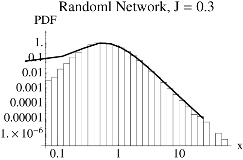
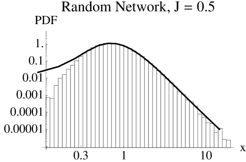
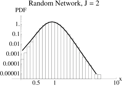
Figure 2: A log-log plot of the PDF on the random network obtained by numerical simulation for $J=0.3$ (left), 0.5 (middle), and 2.0(right).

In Fig. 2 we plot the PDFs obtained by numerical simulation for $J=0.3,0.5$, and 2.0. The PDFs obtained using our theory are indicated by the solid line and show good agreement with the numerical simulation for all $x$ for the $J=2.0$ case, but there are minor discrepancies at small $x$ values in the cases of $J=0.3$ and 0.5. The discrepancy is due to the $Mi\gg\sqrt{S_{i}}$ assumption used for deriving Eqs. (8) and (9). The maximum $S_{i}^{2}$ value calculated by Eqs. (13) and (10) is 0.33 for $J=0.3$ and 0.09 for $J=0.5$, while $M_{i}=1$. Thus, the $M_{i}\gg S_{i}$ approximation is not valid as $\sqrt{S_{i}}$ is larger than 0.3. However, the approximation is valid for the $J=2.0$ case as the maximum $S_{i}^{2}$ value is 0.01.

III.2 Small-World Network

Next, we consider three networks created by the WS algorithm. The networks have $N=100$ nodes and a mean degree of $\langle d\rangle=8$ with different rewiring rates of $p=0.01,0.1$, and 0.2. Fig. 3 shows both the networks and PDFs. In the case of $p=0.01$, our theory differs from the numerical simulation, while we find good agreement for the $p=0.1$ and $p=0.2$ cases.

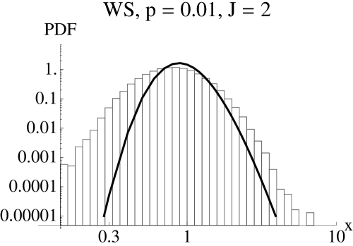
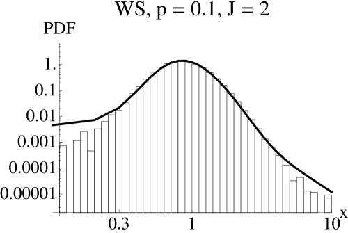
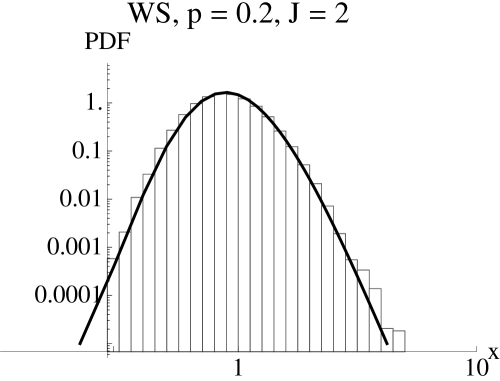
Figure 3: Upper: The small-world networks created by the Watts–Strogatz algorithm with rewiring probabilities of $p=0.01,0.1,$ and 0.2 used to test our theory. Lower: The PDFs obtained from simulations on each networks with $J=2.0$. The solid lines show the results of the method proposed here.

To investigate the reason for this discrepancy, we examine the scatter plots of $x$ and $\bar{x}$ for $p=0.01$ and $p=0.1$ in Fig. 4. For $p=0.01$, we find that there is a strong correlation between $x$ and $\bar{x}$ that weakens for $p=0.1$. The differences can be quantified by the correlation, which is 0.74 for $p=0.01$ and 0.48 for $p=0.1$. This result suggests that the discrepancy is caused by the breakdown of independent assumption.

It is reasonable to question here when and why the independent assumption fails. The small-world property does not appear to affect the independence of wealth because the networks show high-clustering and small betweenness for both the $p=0.01$ and 0.1 cases. We return to this point in the discussion section.

Figure 4: Scatter plots of $x$ and $\bar{x}$ for the BM model on WS networks with $p=0.01$ and 0.1 and with $J=2$.

III.3 American college football network

The American college football network obtained by Girvan and NewmanGirvan includes 115 nodes and 613 edges. The simulated PDFs for $J=0.3$ and 0.5 are shown in Fig. 5. In both cases, our theory reproduces the PDF well.

The agreement between theory and simulation seems excellent. We have not understand the reason for this good agreement, however, one possible reason is that this network has community structure. As Girvan and Newman showed, this network has clear communities. As we will see in the later section, the spatial correlation of wealth would be small for globally coupled network. Therefore it is natural to assume that wealth correlation is also small, if the network is consisted from several densely connected subgraphs. However, we still need further study to explain this excellent agreement.

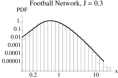
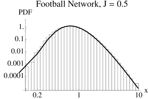
Figure 5: The simulated PDFs of the BM model on the American college football network for $J=0.3$ and 0.5. The solid lines represent the results obtained by our theory.

IV Discussion and Conclusions

Here, we have developed a theory for the BM model on complex networks. By generalizing our previous work, we were able to propose a theory applicable to a complex network with a given adjacency matrix. Using the adiabatic and independent assumptions, we derived the equations that determine the static PDF of the wealth. The result was compared to numerical simulations, and we found our theory works well on a Erdös-Rényi network, WS networks with $p\geq 0.1$, and the American college football network. We also found that the theory did not perform well for a WS network with $p=0.01$ as the independent assumption is no longer valid.

The theory does not apply to a WS network with a small $p$ value because of the large spatial correlation in this case. Thus, we may ask when and why the spatial correlation becomes large. While it is difficult to give a complete answer to this question, the following discussion suggests that the properties of the Laplacian are essential to this problem.

Suppose that $J$ is very large and the fluctuations of $x$ are very small. Under such circumstances, we can approximate $xdW$ in Eq. (1) as $dW$ and obtain

$$dx_{i}=-J\sum_{j}L_{ij}x_{j}dt+\sqrt{2}\sigma dW\;,$$ (14)

where $L=(L_{ij})$ is the Laplacian matrix $L_{ij}=\delta_{ij}d_{i}-a_{ij}$. To investigate the correlation in this toy model, we assume for simplicity that the network is undirected and connected. Introducing the eigenvalues and corresponding normalized eigenvectors of $L$ as $\lambda_{1}=0<\lambda_{2}\leq\cdots\lambda_{N}$ and $\mathbf{v}_{1},\mathbf{v}_{2},\cdots\mathbf{v}_{N}$, we can write $(x_{1},x_{2},\cdots,x_{N})^{T}=\sum_{i=1}^{N}q_{i}\mathbf{v}_{i}$. Then $L$ is diagonalized and Eq. (14) can be written as

$$dq_{i}=-J\lambda_{i}q_{i}dt+\sqrt{2}\sigma dW\;.$$ (15)

The static distribution of $q_{i}(2\leq i\leq N)$ is calculated as

$$P(q_{i})=\frac{\sqrt{J\lambda_{i}}}{\sqrt{2\pi}\sigma}\exp\left[-\frac{J\lambda_{i}q_{i}^{2}}{2\sigma^{2}}\right]\;.$$ (16)

The $q_{1}$ term does not have a static distribution because $\lambda_{1}=0$. However, because $\mathbf{v}_{1}=\frac{1}{\sqrt{N}}(1,1,\cdots,1)$, this term gives the uniform change, $x_{i}\rightarrow x_{i}+C$, and does not contribute to the correlation.

From Eq. (16) and the relation $x_{i}=\sum_{j}q_{j}(\mathbf{v}_{j})_{i}$, we obtain the covariance

$$\langle(x_{i}-\langle x\rangle)(x_{j}-\langle x\rangle)\rangle=\sum_{l=2}^{N}\frac{\sigma^{2}}{J\lambda_{l}}(\mathbf{v}_{l})_{i}(\mathbf{v}_{l})_{j}\;.$$ (17)

Our independent assumption implies that the off-diagonal elements of Eq. (17) are smaller than the diagonal elements. This condition is satisfied if every $\mathbf{v}_{i}$ is ”localized”, in other words, has only one large components. It has been shown by some researchers that eigenvectors is localized in many complex networks McGraw2008 ; Nakao2010 . Our theory will be applicable to these network models.

We also consider here the case for which the adiabatic assumption is not valid. If the node degree is large enough, then $\tilde{x}$ changes at a much slower rate than that of $x$. Therefore, this assumption will be valid if the degree of each node is large. On the other hand, if the degree of each node is small, then not only the adiabatic assumption but also the use of the central-limit theorem cannot be justified. For example, our theory will not work well for the “star”-network in which almost all nodes have a degree of 1.

We note that theory for the BM model in the wealth-condensed phase is still elusive, as the standard central-limit theory is not applicable when $\langle x^{2}\rangle$ diverges. Thus, to discuss the static properties, we will need to generalize the central-limit theorem so that it can be adopted even if the variance diverges.

Finally, we note that our developed technique is applicable to other dynamical systems subject to noise. Stochastic dynamics on complex network is attracting the interests of many reserchers recently, however, dynamics with multiplicative noise has not studied so far. We believe this method will shed new light on other problems regarding the dynamics on complex networks.

References

- (1) R. Pastor-Satorras and A. Vespignani, Phys. Rev. Lett. 86, 3200(2001).
- (2) T. Nishikawa, A. E. Motter, Y.-C Lai, and F. C. Hoppensteadt, Phys. Rev. Lett. 91,014101(2003).
- (3) T. Ichinomiya, Phys. Rev. E 70 026116(2004).
- (4) H. Nakao and A. Mikhaikov, Nature Phys. 6 544(2010).
- (5) J. Bouchaud and M. Mézard, Physica A 282 536 (2000).
- (6) V. Pareto, Cours d’économie politique Macmilan, London 1897.
- (7) D. Garlaschelli and M. I. Loffredo, Physica A. 338 113(2004).
- (8) W. Souma, Y. Fujiwara, and A. Aoyama, arXiv:cond-mat/0108482v1.
- (9) T. Ichinomiya, arXiv:1209.2467v1.
- (10) D. J. Watts and S. H. Strogatz, Nature 393 440 (1998).
- (11) M. Girvan and M. E. J. Newman, Proc. Natl. Acad. Sci. USA 99 7821(2002).
- (12) P. N. McGraw and M. Menzinger, Phys. Rev. E 77, 031102 (2008) .
- (13) H. Nakao and A. Mikhailov, Nature Physics 6 544 (2010).