Abstract

Sparse representation of astronomical images is discussed. It is shown that a significant gain in sparsity is achieved when particular mixed dictionaries are used for approximating these types of images with greedy selection strategies. Experiments are conducted to confirm: i)Effectiveness at producing sparse representations. ii)Competitiveness, with respect to the time required to process large images. The latter is a consequence of the suitability of the proposed dictionaries for approximating images in partitions of small blocks. This feature makes it possible to apply the effective greedy selection technique Orthogonal Matching Pursuit, up to some block size. For blocks exceeding that size a refinement of the original Matching Pursuit approach is considered. The resulting method is termed Self Projected Matching Pursuit, because is shown to be effective for implementing, via Matching Pursuit itself, the optional back-projection intermediate steps in that approach.

1 Introduction

A common first step in most image processing techniques is to map the image onto a transformed space allowing for the reduction in the number of points to represent the image, up to some desired precision. For a significant reduction in the data dimensionality, from say $N$ to $K<N$ points, the image is said to be $K$-sparse in the transformed domain. In addition to the many applications that benefit from sparse representation of information [1, 2, 3, 4, 5], the emerging theory of sampling, called compressive sensing$/$sampling, asserts that sparsity of a representation may also lead to more economical data collection [6, 7, 8, 9, 10]. The relevance of compressive sensing within the context of astronomical data is discussed in [11, 12], where algorithms for signal recovery are advanced and illustrated by these types of data. The usual compressive sensing framework assumes that the signal is sparse in an orthogonal basis or incoherent dictionary, because most of the recovery proofs have been achieved under those conditions. However, recent theoretical results expand the analysis to coherent dictionaries [13, 14], because it is often the case that an approximation is sparser when elements from such a dictionary are used in the decomposition. Alternatively, as shown in [15, 16], high sparsity enables exploitation of the redundancy in the pixel intensity representation of an image, to reduce the image size when encrypted. The success of this technique, termed Encrypted Image Folding (EIF), strongly depends on the sparsity of the image representation. The sparser the representation is the smaller the size of the folded image.

In this Communication we wish to highlight the significant gain in sparsity that may be obtained by releasing the condition of incoherence when designing a dictionary for sparse representation of astronomical images. The problem we address is described as follows:

Given an astronomical image, find its sparse decomposition as a superposition of elementary components, selected from a large redundant set called a dictionary.

It is clear that the success of producing a very sparse representation of an image depends in a large part on the ability to construct appropriate dictionaries from which to select the right elements, frequently called ‘atoms’. Here a mixed dictionary is considered, which will be shown to be suitable for achieving sparse representations of astronomical images. A useful dictionary for this purpose should be capable of sparsely representing two different features; i)fairly smooth regions (nebulae) of intergalactic media, gases, dust, etc., and ii)bright spots (stars). In order to account for smooth regions we use a Redundant Discrete Cosine (RDC) dictionary. The model of bright spots and edges is accomplished by the union of B-spline dictionaries of different order and support. The combination of these two types of dictionaries provides us with a mixed dictionary yielding a very significant gain in the sparsity of an astronomical image, in relation to the outcomes from the most commomly used transformations in image processing; the Discrete Cosine Transform (DCT) and Discrete Wavelet Transform (DWT). Their convenient distinctive feature is that they are suitable for processing large images by segmenting them into small blocks. The advantage of this property is twofold: a)It entails storage requirements which are affordable for processing by effective pursuit strategies. b)The sequential processing of blocks is fast enough to be practical and there is also room for the possibility of straightforward parallel processing when those resources become widely available.

The numerical experiments for illustrating the approach involve large images from the European Southern Observatory (ESO) [17] and a set of fifty five images captured by the Hubble Space Telescope (HST) [18]. Considerations are restricted to approximations of high quality (PSNR of 45 dB or higher). While the sparsity level strongly depends on each particular image, in all the cases is massively higher than the sparsity yielded by the DCT and DWT. Since the computational time is very competitive, we confidently conclude that the mixed dictionaries under consideration are suitable for achieving highly sparse representation of astronomical images.

The paper is organized as follows: Sec. 2 discusses highly nonlinear approximation techniques and introduces the discrete B-spline based dictionaries which, together with the RDC dictionary, form the highly coherent mixed dictionary that provides the basic elements for representing an image. Matching Pursuit like selection techniques are also discussed in this section. In particular, the proposed Self Projected Matching Pursuit strategy is established as a possible alternative to Orthogonal Matching Pursuit, when the latter cannot be implemented due to storage requirements. Sec. 3 illustrates the capability and effectiveness of the approach to yield fast sparse representation of astronomical images. The conclusions are presented in Sec. 4.

2 Sparse representation by highly nonlinear approximation techniques

We start by introducing some basic notation: $\mathbb{R}$ and $\mathbb{N}$ represent the sets of real and natural numbers, respectively. Boldface letters are used to indicate Euclidean vectors or matrices, whilst standard mathematical fonts indicate components, e.g., $\mathbf{d}\in\mathbb{R}^{N}$ is a vector of components $d(i),\,i=1,\ldots,N$ and $\mathbf{I}\in\mathbb{R}^{N_{x}\times N_{y}}$ a matrix of elements $I(i,j),\,i=1,\ldots,N_{x},\,j=1,\ldots,N_{y}$.

Let $\mathcal{D}=\{\mathbf{d}_{n}\in\mathbb{R}^{N}\}_{n=1}^{M}$ be a spanning set for an inner product space $\mathbb{V}_{N}$ of finite dimension $N$ and $\mathbf{f}\in\mathbb{R}^{N}$ a signal to be approximated by an element $\mathbf{f}^{K}\in\mathbb{V}_{K}={\mbox{\rm{span}}}\{\mathbf{d}_{\ell_{i}}\}_{i=1}^{K}$, i.e.,

$$\mathbf{f}^{K}=\sum_{i=1}^{K}c(i)\mathbf{d}_{\ell_{i}},\text{where}\quad K<N.$$ (1)

When $N=M$ and the spanning set $\mathcal{D}$ is linearly independent it is a basis for $\mathbb{V}_{N}$, otherwise it is a redundant frame [19]. In order to advance in the discussion as to how to select from $\mathcal{D}$ the $K$-elements $\mathbf{d}_{\ell_{i}},\,i=1,\ldots,K$ in (1), we need to discriminate two different situations:

• $M=N$ and $\{\mathbf{d}_{i}\}_{i=1}^{M}$ is an orthogonal basis for $\mathbb{V}_{N}$.

• $K<N$ and $\{\mathbf{d}_{i}\}_{i=1}^{M}$ is a non orthogonal and not necessarily linearly independent spanning set for $\mathbb{V}_{N}$.

Case i) leaves rooms for the linear and nonlinear forms of selecting the elements $\mathbf{d}_{\ell_{i}},\,i=1,\ldots,K$. Both types of approximation are easily realized in practice. A linear procedure determines before hand a fixed order for the elements of $\mathcal{D}$ and uses, say the first $K$ elements, for the approximation. On the contrary, a nonlinear procedure would make the selection dependent on the signal to be approximated. For example: it is well known that in order to construct the approximation $\mathbf{f}^{K}$ of $\mathbf{f}$, such that $\|\mathbf{f}^{K}-\mathbf{f}\|$ is minimum (where $\|\cdot\|$ is the square norm induced by the inner product) one should select the elements $\mathbf{d}_{\ell_{i}},\,i=1,\ldots,K$ corresponding to the $K$ coefficients $c(i)=\langle\mathbf{d}_{\ell_{i}},\mathbf{f}\rangle,\,i=1,\ldots,K$ of largest absolute value. This approximation is nonlinear, but the implementation in finite dimension is straightforward.

On the contrary, case ii) introduces an intractable problem. If $K$ is fixed, the choice of the $K$ elements $\mathbf{d}_{\ell_{i}},\,i=1,\ldots,K$ minimizing $\|\mathbf{f}^{K}-\mathbf{f}\|$ involves a combinatorial problem. Moreover, the alternative situation; the one of finding the minimum value of $K$ such that $\|\mathbf{f}^{K}-\mathbf{f}\|<\rho$, for a given tolerance $\rho$, is also intractable. This is the reason why this type of approximation is said to be highly non linear, and in practice is addressed in some suboptimal manner. Rather than looking for the sparsest solution (minimum value of $K$) one looks for a ‘sparse enough solution’. This means that the number of $K$-terms in (1) is ‘small enough’ for the representation to be convenient in the particular context.

Usually highly non linear approximations of a signal $\mathbf{f}$ using a dictionary $\mathcal{D}=\{\mathbf{d}_{i}\}_{i=1}^{M}$ are realized by:

• Expressing $\mathbf{f}^{K}$ as $\sum_{i=1}^{M}c(i)\mathbf{d}_{i}$ and finding $K$-nonzero coefficients by minimization of the 1-norm $\|\mathbf{c}\|_{1}=\sum_{i=1}^{M}|c(i)|$ [20].

• Using a greedy pursuit strategy for stepwise selection of the $K$ normalized to unity elements $\mathbf{d}_{\ell_{i}}\,i=1,\ldots,K$, called atoms, for producing the approximation $\mathbf{f}^{K}=\sum_{i=1}^{K}c(i)\mathbf{d}_{\ell_{i}}$, which is termed atomic decomposition.

We restrict considerations to greedy pursuit algorithms because, for the highly coherent dictionaries we are considering, are more effective and faster than those based on minimization of the 1-norm.

2.A Matching Pursuit based selection techniques

The greedy selection strategy Matching Pursuit (MP) was introduced with this name in the context of signal processing by S. Mallat and Z. Zhang [21]. Previously it had appeared as a regression technique in the statistical literature, where the convergence property was established [22]. The implementation is very simple and evolves by successive approximations as follows.

Let $\mathbf{R}^{k}$ be the $k$-th order residue, $\mathbf{R}^{k}=\mathbf{f}-\mathbf{f}^{k}$, and $\ell_{k}$ the index for which the corresponding dictionary atom $\mathbf{d}_{\ell_{k}}$ yields a maximal value of $|\langle\mathbf{d}_{i},\mathbf{R}^{k}\rangle|,\,i=1,\ldots M$. Starting with an initial approximation $\mathbf{f}^{1}=0$ and $\mathbf{R}^{1}=\mathbf{f}$ the algorithm iterates by sub-decomposing the $k$-th order residue into

$$\mathbf{R}^{k}=\langle\mathbf{d}_{n},\mathbf{R}^{k}\rangle\mathbf{d}_{n}+\mathbf{R}^{k+1},\quad n=1,\ldots,M,$$ (2)

which defines the residue at order $k+1$. Since $\mathbf{R}^{k+1}$ given in (2) is orthogonal to all $\mathbf{d}_{n},\,n=1,\ldots,M$, it is true that

$$\|\mathbf{R}^{k}\|^{2}=|\langle\mathbf{d}_{n},\mathbf{R}^{k}\rangle|^{2}+\|\mathbf{R}^{k+1}\|^{2},\quad n=1,\ldots,M.$$ (3)

Hence, the dictionary atom $\mathbf{d}_{\ell_{k}}$ yielding a maximal value of $|\langle\mathbf{R}^{k},\mathbf{d}_{n}\rangle|$ minimizes $\|\mathbf{R}^{k+1}\|^{2}$.

From (2) it follows that at each iteration $k$ the MP algorithm results in an intermediate representation of the form:

$$\mathbf{f}=\mathbf{f}^{k}+\mathbf{R}^{k+1}$$ (4)

with

$$\mathbf{f}^{k}=\sum_{n=1}^{k}\langle\mathbf{d}_{\ell_{n}},\mathbf{R}^{n}\rangle\mathbf{d}_{\ell_{n}}.$$ (5)

It was first proved in [22] that in the limit $k\rightarrow\infty$ the sequence $\mathbf{f}^{k}$ converges to $\hat{P}_{\mathbb{V}_{M}}\mathbf{f}$, the orthogonal projection of $\mathbf{f}$ onto $\mathbb{V}_{M}={\mbox{\rm{span}}}\{\mathbf{d}_{{n}}\}_{n=1}^{M}$ (the proof is translated to the MP context in [21]). Nevertheless, if the algorithm is stopped at the $k$th-iteration, $\mathbf{f}^{k}$ recovers an approximation of $\mathbf{f}$ with an error equal to the norm of the residual $\mathbf{R}^{k+1}$ which, if the selected atoms are not orthogonal, will not be orthogonal to the subspace they span. An additional drawback of the MP approach is that the selected atoms may not be linearly independent.

A refinement to MP, which does yield an orthogonal projection approximation at each step, has been termed Orthogonal Matching Pursuit (OMP) [23]. In addition to selecting only linearly independent atoms, the OMP approach improves upon MP numerical convergence rate and therefore amounts to be, usually, a better approximation of a signal after a finite number of iterations. OMP provides a decomposition of the signal as given by:

$$\mathbf{f}^{k}=\sum_{n=1}^{k}c^{k}(n)\mathbf{d}_{\ell_{n}}+\tilde{\mathbf{R}}^{k},$$ (6)

where the coefficients $c^{k}(n)$ are computed in such a way that it is true that

$$\sum_{n=1}^{k}c^{k}(n)\mathbf{d}_{\ell_{n}}=\hat{P}_{\mathbb{V}_{k}}\mathbf{f},\quad{\text{with}}\quad\mathbb{V}_{k}={\mbox{\rm{span}}}\{\mathbf{d}_{\ell_{n}}\}_{n=1}^{k}.$$

Thus, OMP yields the unique element $\mathbf{f}^{k}\in\mathbb{V}_{k}$ minimizing $\|\mathbf{f}^{k}-\mathbf{f}\|$. The superscript of $c^{k}(n)$ in (6) indicates the dependence of these quantities on the iteration step $k$.

The OMP approach is effective for processing signals up to some dimensionality. It may become prohibitive, because of its storage requirements, when the signal dimension exceed some value. In this respect, MP has the advantage of being suitable for processing very large dimensional signals and, for 2D images, it fully exploits the separability property of dictionaries. Since our mixed dictionaries are adequate for block processing, in general the OMP approach is an appropriate technique. However, one of the aims of the present effort is to study, in a standard personal computer, the dependence of the sparsity of a representation with respect to the block size of an image partition. For this purpose, we are forced to overcome storage requirements of the standard OMP implementations. The goal is achieved by applying the refinement to the MP method proposed in the next section.

2.B Self Projected Matching Pursuit

The seminal paper [21] discusses a possible improvement of the MP approximation by means of back-projection steps, which stands for computing the orthogonal projection of the MP approximation. The authors suggest this could be done by the conjugate gradient method. Unfortunatelly the processing time of that method is not affordable in practice for large dimensional problems, and specially with highly correlated dictionaries. Thus, the question we have tried to answer is:

Since the MP approach converges asymptotically to the orthogonal projection onto the span of the selected atoms, would it be affective to use MP itself to compute the back-projection steps?

Of course there is an increment of step wise complexity but, as the example presented here illustrates, on the whole the refinement may perform better and faster.

The resulting method, that we have termed Self Projected Matching Pursuit (SPMP) evolves as follows. Given a dictionary $\mathcal{D}=\{\mathbf{d}_{n}\}_{n=1}^{M}$ and a signal $\mathbf{f}$, set $S=\{\emptyset\}$ and $\mathbf{R}=\mathbf{f}$. Assuming that the required projection step is of length $p$, implement the algorithm below.

• Apply MP up to step $p$ selecting atoms from dictionary $\mathcal{D}=\{\mathbf{d}_{n}\}_{n=1}^{M}$. Assuming that the distinct selected atoms are $\{\mathbf{d}_{\ell_{n}}\}_{n=1}^{k}$ assign $S\leftarrow S\cup\{\mathbf{d}_{\ell_{n}}\}_{n=1}^{k}$. Set $K$ equal to the cardinality of the updated $S$. Let us denote as $\mathbf{f}^{K}$ the approximation of $\mathbf{f}$ so far and as $\mathbf{R}^{K}$ the residue $\mathbf{R}^{K}=\mathbf{f}-\mathbf{f}^{K}$.

• Approximate $\mathbf{R}^{K}$ using only the selected set $S$ as the dictionary, which guarantees the asymptotic convergence to the approximation $\hat{P}_{\mathbb{S}}{\mathbf{R}^{K}}$ of $\mathbf{R}^{K}$, where $\mathbb{S}={\mbox{\rm{span}}}\,S$, and a residue $\mathbf{R}^{\perp}={\mathbf{R}^{K}}-\hat{P}_{\mathbb{S}}\mathbf{R}^{K}$ having no component in $\mathbb{S}$.

• Set $\mathbf{R}\leftarrow\mathbf{R}^{\perp}$ and $\mathbf{f}^{K}\leftarrow\mathbf{f}^{K}+\hat{P}_{\mathbb{S}}\mathbf{R}$ and repeat steps i) and ii) until, for a required $\rho$, the condition $\|\mathbf{R}\|<\rho$ is reached.

For $p=1$ the above refinement gives, asymptotically, the orthogonal projection approximation at each iteration, thereby reproducing the results of OMP. As illustrated by the example below, significant improvement upon the original MP approach may be achieved for values of $p$ larger than one.

Example. This numerical example is a hard test for MP. Consider the Redundant Discrete Cosine (RDC) dictionary $\mathcal{D}_{1}$ given by:

$$\mathcal{D}_{1}=\{\mathbf{v}_{i};\,v_{i}(j)=w_{i}\cos(\frac{\pi(2j-1)(i-1)}{2M}),\,j=1,\ldots,N\}_{i=1}^{M},$$ (7)

with $w_{i},\,i=1,\ldots,M$ normalization factors. For $M=N$ this set is a Discrete Cosine (DC) orthonormal basis for the Euclidean space $\mathbb{R}^{N}$. For $M=2zN$, with $z\in\mathbb{N}$, the set is a RDC dictionary with redundancy $2z$, which will be fixed equal to 2.

Fig. 1: Chirp signal approximated up to error $\rho=0.001\|\mathbf{f}\|$ by i) $K=683$ orthogonal DC components taken from (7) with $N=M=2000$. ii) $K=286$ atoms taken from (7) with $M=2N=4000$ using OMP or $K=1638$ using MP . iii) $K=300$ atoms taken from (7) with $M=2N=4000$ using SPMP with $p=10$ or $K=286$ with $p=3$.

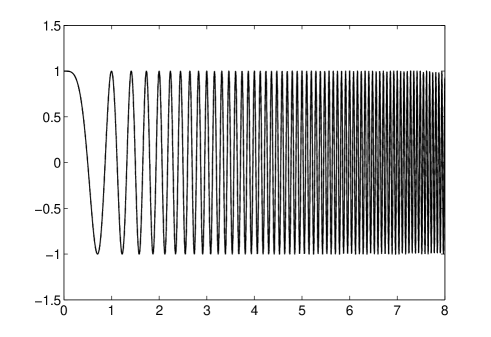
To represent the chirp signal $\cos(2\pi t^{2})$ depicted in Fig. 1 we take an equidistant partition of the interval $[0,8]$ consisting of $N=2000$ points and sample the chirp at those points $f(i),\,i=1,\ldots,N$. The aim is to find an approximation of these points up to precision $\rho=0.001\|\mathbf{f}\|$. Considering $M=N=2000$ in the above definition of $\mathcal{D}_{1}$ we have an orthonormal basis and therefore both MP and OMP methods give the sparsest decomposition of the signal in orthogonal DC components. For an approximation to the given precision (coinciding visually with the theoretical chirp in Fig. 1) it is necessary to use $K=683$ orthogonal elements from (7). Now, setting $M=2N=4000$ the dictionary $\mathcal{D}_{1}$ is no longer an orthogonal basis but a redundant tight frame [19] and the algorithms MP and OMP produce very different decompositions. While OMP improves the sparsity of the representation requiring only $K=286$ components, MP needs $K=1638$ different atoms, i.e. significantly more than with the orthonormal basis. The reason for the poor performance of MP is that in the redundant dictionary the atoms are highly correlated and the method is picking linearly dependent atoms, something that cannot occur with OMP. However, when applying the proposed refinement SPMP with projection step $p=10$ the number of required components drops to $K=300$. For $p=3$ the number of required components is that of OMP, i.e. $K=286$. While in this example there is no need for the SPMP approach, because the already established algorithm OMP performs the decomposition faster, the result illustrates the fact that SPMP can provide an effective alternative to OMP when, as is the case with 2D images, OMP becomes slow or its storage demands cannot be met. Further details for the 2D implementation of SPMP will be discussed in Sec. 2.C. Before that, we shall introduce the proposed mixed dictionaries for representing astronomical images.

2.B.1 Building mixed dictionaries for sparse representation of astronomical images

Assume that the $K$-sparse representation of a given image $\mathbf{I}\in\mathbb{R}^{N_{x}\times N_{y}},\,$ $N_{x},N_{y}\in\mathbb{N}$, is represented as

$$\mathbf{I}^{K}=\sum_{i=1}^{K}c^{K}(i)\mathbf{D}_{\ell_{i}},$$ (8)

where the elements $\mathbf{D}_{\ell_{i}}\in\mathbb{R}^{N_{x}\times N_{y}},\,i=1,\ldots,K$ in (8), are to be selected from a dictionary $\mathcal{D}=\{D_{i}\}_{i=1}^{M}$ which is obtained as the Kronecker product $\mathcal{D}=\mathcal{D}^{x}\otimes\mathcal{D}^{y}$ of the dictionaries $\mathcal{D}^{x}=\{\mathbf{d}^{x}_{n}\in\mathbb{R}^{N_{x}}\}_{n=1}^{M_{x}}$ and $\mathcal{D}^{y}=\{\mathbf{d}^{y}_{m}\in\mathbb{R}^{N_{y}}\}_{m=1}^{M_{y}}$. In this section we discuss a particular dictionary $\mathcal{D}$, which will be shown to be adequate for sparse representation of astronomical images.

Redundant Discrete Cosine (RDC) Dictionary

As already mentioned in order to sparsely represent the fairly smooth regions of the images being considered, one of the components of the proposed mixed dictionary is chosen to be a RDC dictionary $\mathcal{D}_{1}$ introduced in the last section, fixing $M=2N$ so as to have a RDC dictionary with redundancy two.

Redundant Discrete B-Spline (RDBS) based dictionaries

The other component of the proposed mixed dictionary, which allows for the representation of bright spots and edges, is inspired by a general result holding for continuous spline spaces. Namely, that spline spaces on a compact interval can be spanned by dictionaries of B-splines of broader support than the corresponding B-spline basis functions [26, 27]. This may result in a very considerable gain in sparsity for functions well approximated in spline spaces. Here we consider equally spaced knots so that the corresponding B-splines are called cardinal. All the cardinal B-splines of order $m$ can be obtained from one cardinal B-spline $B(x)$ associated with the uniform simple knot sequence $\Delta=0,1,\dots,m$. Such a function is given as [28]

$$B_{m}(x)=\frac{1}{m!}\sum_{i=0}^{m}(-1)^{i}\binom{m}{i}(x-i)^{m-1}_{+},$$ (9)

where $(x-i)^{m-1}_{+}$ is equal to $(x-i)^{m-1}$ if $x-i>0$ and 0 otherwise. We shall consider only B-Splines of order $m=2$ and $m=4$ and include associated derivatives. For $m=2$ the corresponding space is the space of piece wise linear functions and can be spanned by a linear B-spline basis, or dictionaries of broader support, arising by translating a prototype ‘hat’ function. Equivalently, the cubic spline space corresponding to $m=4$ is spanned by the usual cubic B-spline basis, or dictionaries of cubic B-spline functions of broader support. Details on how to build B-spline dictionaries are given in [26, 27]. The numerical construction of the cases $m=2$ and $m=4$ considered here is very simple and arises by translations of the prototype functions given below:

$$B^{l}_{2}(x)= \frac{x}{l} 0\leq x<l$$ if (10a)

$$B^{l}_{2}(x)= 2-\frac{x}{l} l\leq x<2l$$ if (10b)

$$B^{l}_{2}(x)= 0$$ otherwise. (10c)

$$B^{l}_{4}(x)= \frac{x^{3}}{6l^{3}} 0\leq x<l$$ if (11a)

$$B^{l}_{4}(x)= -\frac{x^{3}}{2l^{3}}+2\frac{x^{2}}{l^{2}}-2\frac{x}{l}+\frac{2}{3} l\leq x<2l$$ if (11b)

$$B^{l}_{4}(x)= \frac{x^{3}}{2l^{3}}-4\frac{x^{2}}{l^{2}}+10\frac{x}{l}-\frac{22}{3} 2l\leq x<3l$$ if (11c)

$$B^{l}_{4}(x)= -\frac{x^{3}}{6l^{3}}+2\frac{x^{2}}{l^{2}}-8\frac{x}{l}+\frac{32}{3} 3l\leq x<4l$$ if (11d)

$$B^{l}_{4}(x)= 0$$ otherwise. (11e)

The B-spline basis for the cardinal spline space corresponding to $m=2$ is constructed by considering $l=1$ in (10c) and translating the prototype every knot. Dictionaries for the identical space of functions of broader support arise by setting $l\in\mathbb{N}$ in order to fix the desired support. The B-spline basis for the cubic cardinal spline space, corresponding to $m=4$, requires to set $l=1$ in (11e) and translate the concomitant prototype. Dictionaries are obtained by taking larger values of $l$.

As discussed below, derivatives of the above functions also provide suitable prototypes to achieve higher levels of sparsity in the representation of a signal. Now, for constructing dictionaries for digital image processing we need to

• Discretize the functions to obtain adequate Euclidean vectors.

• Restrict the functions to intervals which allows images to be approximated in small blocks.

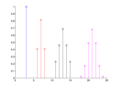
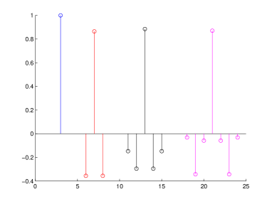
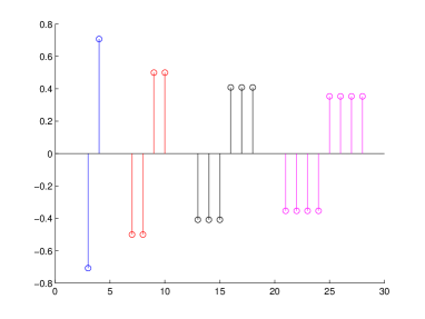
We carry out the discretization by taking the value of a prototype function only at the knots (c.f. small circles in graphs Fig. 2) and translating the prototype one sampling point at each translation step. At the boundaries we apply the ‘cut off’ approach and keep all the vectors whose support has nonzero intersection with the interval being considered.

Remark 1.

It is worth mentioning that by the proposed discretization the hat B-spline basis for the corresponding interval becomes the standard Euclidean basis. By discretizing the hats of broader support the samples preserve the hat shape.

Obviously for a finite dimension Euclidean space one can construct arbitrary dictionaries. In particular, redundant B-spline based dictionaries with prototypes of different support and shapes arising from the functions (10c) and (11e) and their corresponding derivatives.

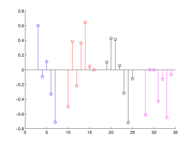
Indicating as ${\rm{d}}^{1}B^{l}_{m}(x)$ the derivative of $B^{l}_{m}(x)$ and as ${\rm{d}}^{2}B^{l}_{m}(x)$ its second derivative, in addition to linear and cubic B-splines we shall consider the additional prototypes ${\rm{d}}^{1}B^{l}_{2}(x),\,{\rm{d}}^{1}B^{l}_{4}(x)$ and ${\rm{d}}^{2}B^{l}_{4}(x)$. Vectors of different support may be included by merging those dictionaries. For our experiments we construct the Redundant Discreet B-Spline (RDBS) based dictionaries as follows:

$$\mathcal{D}_{s}=\{b_{i}Y^{s}_{m}(j-i)|N;j=1,\ldots,L\}_{i=1}^{M_{s}},\quad m=2,4,\,s=2,\ldots,9,$$

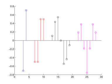
where the notation $Y_{m}(j-i)|N$ indicates the restriction to be an array of size $N$ and $b_{i},\,i=1,\ldots,M_{s}$ are normalization constants. The arrays $Y^{s}_{2},\,s=2,3,4,\,Y^{7}_{4}$, shown consecutively in the left graph of Fig. 2, and $Y^{s}_{2},\,s=5,6,\ Y^{s}_{4},s=8,9$ shown consecutively in the right graph of the same figure, are defined as follows:

$$Y^{s}_{2}= B^{l}_{2},\,l=1,2,3$$ for  s=2,3,4  (respectively) (12a)

$$Y^{s}_{2}= {\rm{d}}^{1}B^{l}_{2},\,l=2,3$$ for  s=5,6  (respectively). (12b)

$$Y^{s}_{4}= B^{2}_{4}$$ for s=7 (13a)

$$Y^{s}_{4}= {\rm{d}}^{1}B^{2}_{4}$$ for s=8 (13b)

$$Y^{s}_{4}= {\rm{d}}^{2}B^{2}_{4}$$ for s=9. (13c)

Fig. 2: Prototype atoms as defined in (12b) and (13c). The RDBS component of the dictionary is constructed by translation or these atoms, applying the cut off approach at the boundaries.

The cut off approach applied to the boundaries implies that the numbers $M_{s}$ of total atoms in the $s$th-dictionary varies according to the atom’s support.

Taking $N=N_{x}$, an unidimensional mixed dictionary, $\mathcal{D}^{x}$, results by joining dictionary $\mathcal{D}_{1}$ (c.f. (7)) and the above defined RDBS ones, i.e. $\mathcal{D}^{x}=\cup_{s=1}^{9}\mathcal{D}_{s},$. Taking $N=N_{y}$ an equivalent mixed dictionary, $\mathcal{D}^{y}$, is obtained. The mixed dictionary $\mathcal{D}$ for $\mathbb{R}^{N_{x}\times N_{y}}$ is the Kronecker product $\mathcal{D}=\mathcal{D}^{x}\otimes\mathcal{D}^{y}$. However, as discussed below, this 2D dictionary does not need to be constructed. This advantage represents a huge save in memory requirements.

2.C 2D implementation of the selection strategies with separable dictionaries

Given an image $\mathbf{I}\in\mathbb{R}^{{N_{x}\times N_{y}}}$ and two 1D dictionaries $\mathcal{D}^{x}=\{\mathbf{d}^{x}_{n}\in\mathbb{R}^{N_{x}}\}_{n=1}^{M_{x}}$ and $\mathcal{D}^{y}=\{\mathbf{d}^{y}_{m}\in\mathbb{R}^{N_{y}}\}_{m=1}^{M_{y}}$ the greedy procedure OMP2D for approximating $\mathbf{I}$ with atoms taken from $\mathcal{D}^{x}$ and $\mathcal{D}^{y}$ iterates as follows.

On setting $\mathbf{R}^{0}=\mathbf{I}$ at iteration $k+1$ the algorithm selects the atoms $\mathbf{d}^{x}_{\ell^{x}_{k+1}}\in\mathcal{D}^{x}$ and $\mathbf{d}^{y}_{\ell^{y}_{k+1}}\in\mathcal{D}^{y}$ that maximize the absolute value of the Frobenius inner products $\langle\mathbf{d}^{x}_{n},\mathbf{R}^{k}\mathbf{d}^{y}_{m}\rangle_{\mathrm{F}},\,n=1,\ldots,M_{x},\,m=1,\ldots,M_{y},$ i.e.,

$$\begin{split}{{{\ell}^{x}}_{k+1},{{\ell}^{y}}_{k+1}}&=\operatorname*{arg\,max}_{\begin{subarray}{c}n=1,\ldots,M_{x}\\ m=1,\ldots,M_{y}\end{subarray}}|\sum_{\begin{subarray}{c}i=1\\ j=1\end{subarray}}^{{N_{x},N_{y}}}d^{x}_{n}(i)R^{k}(i,j)d^{y}_{m}(j)|\\ \text{with}\\ R^{k}(i,j)&=I(i,j)-\sum_{n=1}^{k}c^{k}(n)d^{x}_{\ell^{x}_{n}}(i)d^{y}_{\ell^{y}_{n}}(j).\end{split}$$ (14)

The coefficients $c^{k}(n),\,n=1,\ldots,k$ in the above expansion are such that $\|\mathbf{R}^{k}\|_{\mathrm{F}}$ is minimum, where $\|\cdot\|_{\mathrm{F}}$ is the Frobenius norm. This is ensured by requesting that $\mathbf{R}^{k}=\mathbf{I}-\hat{P}_{\mathbb{V}_{k}}\mathbf{I}$, where $\hat{P}_{\mathbb{V}_{k}}$ is the orthogonal projection operator onto $\mathbb{V}_{k}={\mbox{\rm{span}}}\{\mathbf{d}^{x}_{\ell^{x}_{n}}\otimes\mathbf{d}^{y}_{\ell^{y}_{n}}\}_{n=1}^{k}$. A straightforward generalization of the implementation discussed in [24, 25] for the 1D case provides us with the representation of $\hat{P}_{\mathbb{V}_{k}}\mathbf{I}$ as given by

$$\hat{P}_{\mathbb{V}_{k}}\mathbf{I}=\sum_{n=1}^{k}\mathbf{A}_{n}\langle\mathbf{B}_{n}^{k},\mathbf{I}\rangle_{F}=\sum_{n=1}^{k}c^{k}(n)\mathbf{A}_{n},$$ (15)

where each $\mathbf{A}_{n}\in\mathbb{R}^{{N_{x}\times N_{y}}}$ is an array with the selected atoms $\mathbf{A}_{n}=\mathbf{d}^{x}_{\ell^{x}_{n}}\otimes\mathbf{d}^{y}_{\ell^{y}_{n}}$ and $\mathbf{B}_{n}^{k},\,n=1,\ldots,k$ are the concomitant reciprocal matrices, which are the unique elements of $\mathbb{R}^{{N_{x}\times N_{y}}}$ satisfying the conditions:

• $\langle\mathbf{A}_{n},\mathbf{B}_{m}^{k}\rangle_{\mathrm{F}}=\delta_{n,m}=\begin{cases}1&\mbox{if}\,n=m\\ 0&\mbox{if}\,n\neq m.\end{cases}$

• ${\mathbb{V}_{k}}={\mbox{\rm{span}}}\{\mathbf{B}_{n}^{k}\}_{n=1}^{k}.$

Such matrices can be adaptively constructed through the recursion formula:

$$\begin{split}\mathbf{B}_{n}^{k+1}&=\mathbf{B}_{n}^{k}-\mathbf{B}_{k+1}^{k+1}\langle\mathbf{A}_{k+1},\mathbf{B}_{n}^{k}\rangle_{\mathrm{F}},\quad n=1,\ldots,k\\ \text{where}\\ \mathbf{B}_{k+1}^{k+1}&=\mathbf{C}_{k+1}/\|\mathbf{C}_{k+1}\|_{\mathrm{F}}^{2},\,\,\text{with}\,\,\mathbf{C}_{1}=\mathbf{A}_{1}\,\,\text{and}\,\,\mathbf{C}_{k+1}=\mathbf{A}_{k+1}-\sum_{n=1}^{k}\frac{\mathbf{C}_{n}}{\|\mathbf{C}_{n}\|_{\mathrm{F}}^{2}}\langle\mathbf{C}_{n},\mathbf{A}_{k+1}\rangle_{\mathrm{F}}.\end{split}$$ (16)

For numerical accuracy in the construction of the set $\mathbf{C}_{n},\,n=1,\ldots,k+1$ at least one re-orthogonalization step is usually needed. It implies that one needs to recalculate these matrices as

$$\mathbf{C}_{k+1}=\mathbf{C}_{k+1}-\sum_{n=1}^{k}\frac{\mathbf{C}_{n}}{\|\mathbf{C}_{n}\|_{\mathrm{F}}^{2}}\langle\mathbf{C}_{n},\mathbf{C}_{k+1}\rangle_{\mathrm{F}}.$$ (17)

The coefficients in (15) are obtained from the inner products $c^{k}(n)=\langle\mathbf{B}_{n}^{k},\mathbf{I}\rangle_{\mathrm{F}},\,n=1,\ldots,k$. The algorithm iterates up to step, say $K$, for which, for a given $\rho$, the stopping criterion $\|\mathbf{I}-\mathbf{I}^{K}\|_{\mathrm{F}}<\rho$ is met. The MATLAB function OMP2D, and corresponding MEX file in C++ for faster implementation of the identical function, are available at [29].

Up to some block-size OMP2D is very effective. It takes advantage of the separability property of the dictionary, except for the construction of the required matrices $\mathbf{B}_{n}^{k},\,n=1,\ldots,k$. Unfortunately, for blocks larger than a certain size the concomitant storage demands are not available on a standard personal computer, or the computations became very slow and the above implementation of OMP2D is no longer affective. As already mentioned, in order to avoid the storage and computation of matrices $\mathbf{B}_{n}^{k},\,n=1,\ldots,k$, we propose the SPMP method. Algorithms 1, 2, and 3 outline its implementation in 2D, which we term SPMP2D.

  Input: Image $\mathbf{I}\in\mathbb{R}^{N_{x}\times N_{y}}$. Dictionaries $\mathcal{D}^{x}=\{\mathbf{d}^{x}_{n}\in\mathbb{R}^{N_{x}}\}_{n=1}^{M_{x}}$ and $\mathcal{D}^{y}=\{\mathbf{d}^{y}_{n}\in\mathbb{R}^{N_{y}}\}_{n=1}^{M_{y}}$.Approximation error $\rho>0$ and tolerance $\epsilon>0$ for the numerical realization of the projection. Length of projection step $p$.

  Output: Approximated image $\mathbf{I}_{\rm{Approx}}\in\mathbb{R}^{N_{x}\times N_{y}}$. Coefficients in the atomic decomposition $\mathbf{c}\in\mathbb{R}^{k}$. Ordered pair of indices labeling the selected atoms $\Gamma=\{(\ell^{x}_{n},\ell^{y}_{n})\}_{n=1}^{K}$.

  { Initialization}

  Set$\,\,\Gamma\,=\,\{\emptyset\},\quad\mathbf{I}_{\rm{Approx}}\,=\,0,\quad\mathbf{R}\,=\,\mathbf{I}\,\quad k\,=\,0,\quad{\rm{Error}_{1}}=2\rho$

  Set$\,\,C(i,j)\,=\,0,\,i\,=\,1,\ldots,M_{x},\,j\,=\,1,\ldots,M_{y}.$

  { Begin the algorithm}

  while ${\rm{Error}_{1}}>\rho$ do

     Apply Algorithm 2 {p-MP-iterations} to obtain:

     $\Gamma=\{(\ell^{x}_{n},\ell^{y}_{n})\}_{n=1}^{k},\mathbf{I}_{\rm{Approx}}\in\mathbb{R}^{N_{x}\times N_{y}},\,\mathbf{R}=\mathbf{I}-\mathbf{I}_{\rm{Approx}}\in\mathbb{R}^{N_{x}\times N_{y}}$ and $\mathbf{C}\in\mathbb{R}^{M_{x}\times M_{y}}$

     { Collect nonzero coefficients in $\mathbf{c}\in\mathbb{R}^{k}$}

     for $n=1:k$ do

        $c(n)=C(\ell^{x}_{n},\ell^{y}_{n})$

     end for

     Apply Algorithm  3 { Improve approximation by orthogonal projection via MP } to update $\mathbf{c}\in\mathbb{R}^{k}$ so that $\mathbf{I}_{\rm{Approx}}\leftarrow\mathbf{I}_{\rm{Approx}}+\hat{P}_{\mathbb{V}_{k}}\mathbf{R}$,  $\mathbf{R}\leftarrow\mathbf{R}-\hat{P}_{\mathbb{V}_{k}}\mathbf{R}$ {where $\mathbb{V}_{k}={\mbox{\rm{span}}}\{\mathbf{d}^{x}_{\ell^{x}_{n}}\otimes\mathbf{d}^{y}_{\ell^{y}_{n}}\}_{n=1}^{k}$}

     for $n=1:k$ do

        $C(\ell^{x}_{n},\ell^{y}_{n})=c(n)${Update of matrix with coefficients}

     end for

     ${\rm{Error}_{1}}\leftarrow\|\mathbf{I}-\mathbf{I}_{\rm{Approx}}\|_{F}$

  end while

Algorithm 1 Implementation of the proposed SPMP2D method to approximate an image.

  for $t=1:p$ do

     for $n=1:M_{x}$ and $m=1:M_{y}$ do

        $G(n,m)=\sum_{\begin{subarray}{c}i=1\\ j=1\end{subarray}}^{N_{x},N_{y}}{d}^{x}_{n}(i)R(i,j){d}^{y}_{m}(j)$

     end for

     ${q^{x},q^{y}}=\arg\max\limits_{n,m=1,\ldots,M}|G(n,m)|$ {MP selection of atoms}

     {Store coefficients as a matrix adding contributions from repeated atoms}

     $C(q^{x},q^{y})=C(q^{x},q^{y})+G(q^{x},q^{y})$

     {Update of approximation and residual}

     for $i=1:N_{x}$ and $j=1:N_{y}$ do

        $\Delta=C(q^{x},q^{y}){d}^{x}_{q^{x}}(i){d}^{y}_{q^{y}}(j)$

        $R(i,j)=R(i,j)-\Delta$

        $I{{}_{\text{Approx}}}(i,j)=I_{\text{Approx}}(i,j)+\Delta$

     end for

     if $(q^{x},q^{y})\notin\Gamma$ then

        $k\leftarrow k+1,\quad(\ell^{x}_{k},\ell^{y}_{k})\leftarrow(q^{x},q^{y}),\quad\Gamma\leftarrow\Gamma\cup(\ell^{x}_{k},\ell^{y}_{k})$ {Update set of indices}

     end if

  end for

Algorithm 2 $p$-plain MP iterations for atoms selection and collection of contributions of repeated atoms

  Set $\,\,{\rm{Error}_{2}}=2\epsilon$

  while ${\rm{Error}_{2}}>\epsilon$ do

     for $n=1:k$ do

        $g(n)=\sum_{\begin{subarray}{c}i=1\\ j=1\end{subarray}}^{N_{x},N_{y}}d^{x}_{\ell^{x}_{n}}(i)R(i,j)d^{y}_{\ell^{y}_{n}}(j)$

     end for

     ${q}=\arg\max\limits_{n=1,\ldots,k}|g(n)|$

     $c(q)=c(q)+g(q)$ {Update coefficients}

     {Update approximation and residual}

     for $i=1:N_{x}$ and $j=1:N_{y}$ do

        $\mathrm{R}(i,j)=\mathrm{R}(i,j)-{d}^{x}_{\ell^{x}_{q}}(i){d}^{y}_{\ell^{y}_{q}}(j)g(q)$

        $\mathrm{I}{{}_{\text{Approx}}}(i,j)=\mathrm{I}{{}_{\text{Approx}}}(i,j)+{d}^{x}_{\ell^{x}_{q}}(i){d}^{y}_{\ell^{y}_{q}}(j)g(q)$

     end for

     ${\rm{Error}_{2}}\leftarrow|g(q)|$

  end while

Algorithm 3 Orthogonal projection onto $\mathbb{V}_{k}={\mbox{\rm{span}}}\{\mathbf{d}^{x}_{\ell^{x}_{n}}\otimes\mathbf{d}^{y}_{\ell^{y}_{n}}\}_{n=1}^{k}$ via MP

Putting aside the complexity for the selection process, which is the same for both approaches, the complexity order for the procedure of including one more term in the approximation is

• O$(kN_{x}N_{y})$ for OMP2D

• O$(k\kappa N_{x}N_{y})$ for SPMP2D, where $\kappa$ indicates the number of iterations to improve the MP2D approximation by self projections.

The number $\kappa$ is expected to depend on the correlation of the selected atoms. For the dictionaries and the class of images we are considering we can assert that $\kappa$ is a small number. When this relation is fulfilled the complexity of both approaches are of equivalent order. However, as illustrated in the next section, the storage requirements of OMP2D slow the processing significantly when the size of the blocks partitioning the images increases beyond some value. In such situations SPMP2D, which does not require the calculation or storage of Kronecker products, becomes a suitable alternative for orthogonalization of the MP approach.

3 Numerical Experiments and Results

The viability of using the mixed dictionary described in Section 2.B.1 to quickly approximate an image by either OMP2D or SPMP2D follows from its suitability for block processing. This implies to divide the image $\mathbf{I}$ into small blocks, for independent approximation.

Without loss of generality blocks are assumed to be square of size $N_{h}\times N_{h}$ pixels. Also for simplicity an image $\mathbf{I}$ will be assumed to be the composition of $H$ identical blocks, i.e.,

$$\mathbf{I}=\cup_{h=1}^{H}\mathbf{I}_{h},$$

where every $\mathbf{I}_{h}$ is an intensity array of size ${N_{h}}\times N_{h}$, to be approximated as

$$I^{K_{h}}(i,j)=\sum_{n=1}^{K_{h}}c^{K_{h}}(n){d}^{x}_{\ell^{x}_{n}}(i){d}^{y}_{\ell^{y}_{n}}(j),\quad i,j=1,\ldots N_{h}.$$ (18)

In what follows the performance of our dictionary based approach is illustrated by recourse to numerical experiments. The sparsity is measured by the Sparsity Ratio (SR) defined as

$$\text{SR}=\frac{\text{number of pixels}}{\text{number of coeffients}}=\frac{HN_{h}^{2}}{\sum_{h=1}^{H}{K_{h}}}.$$

General setup

The experiments have been realized in the MATLAB programming environment, on a laptop with a 2.4GHz Intel Core 2 Duo P8600 processor and 7.7GB of RAM.

In all the cases the approximation tolerance is fixed to produce a sharp PSNR of 45dB for the complete image. For such a PSNR Mean Structure Similarity index (MSSIM) [30] with respect to the original image is very close to one (MSSIM $>0.98$ for all the images).

Unless explicitly specified the mixed dictionary is the one introduced in section Sec.2.B.1, i.e. the union of a RDC dictionary, redundancy two, and the RDBS dictionary arising by translation of the eight prototypes shown in Fig. 2.

The comparison with the DCT and DWT refers to the nonlinear approach achieving, by thresholding of the DCT and DWT coefficients respectively, the required PSNR of 45 dB. The DWT is applied to the whole image using software implementing the Cohen-Daubechies-Feauveau 9$/$7 wavelet transform.

Experiment I

The aim is to evaluate the sparsity of an image representation, by the proposed mixed dictionary, against the size of the blocks partitioning the image. The results are compared with those yielded by the 2D version of the DCT and DWT orthogonal transforms. With this end in mind, numerical experiments were conducted using a set of images downloaded from the ESO website [17], converted to gray intensity levels, for two resolutions (publication and screen size). We include here full results corresponding to the two images in Fig. 3, which are good representatives of the range of images in the data set tested.

Fig. 3: The first image is the Nebula Orion (Messier 42 Ref. eso1006) and the second the Spiral Galaxy NGC 4945 Ref. eso0931). Both images are taken from ESO [17] at publication and screen resolutions. The corresponding sizes (in pixels) are: $4000\times 3252$ and $1280\times 1574$ (nebula) $4000\times 4000$ and $1280\times 1280$ (galaxy).

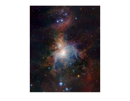
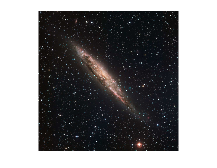
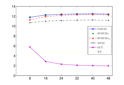
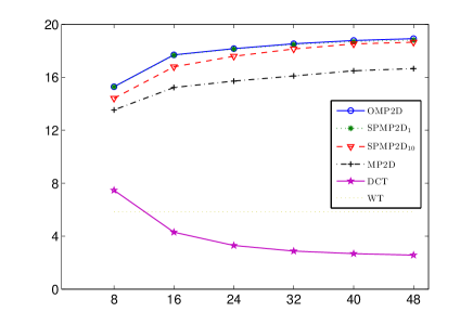
For a fixed PSNR of 45dB the SR is calculated by partitioning the corresponding image into square blocks of side length $8,16,24,32,40$ and $48$. Fig. 4 depicts the SR obtained, using the mixed dictionaries from Sec. 2.B.1, and OMP2D, SPMP2D with projection step one (SPMP2D₁) and ten (SPMP2D₁₀), and the 2D version of MP, for separable dictionaries, that we denote MP2D. Sparsity is also compared against results for the DCT (for the same block size) and the DWT applied to the whole image.

Fig. 4: SR vs partition of side length $8,16,24,32,40$, and 48 yielded by OMP2D, SPMP2D with projection step one (SPMP2D₁) and ten (SPMP2D₁₀), MP2D, and the DCT. The constant dotted line corresponds to the DWT result and is plotted only for visual comparison, since the DWT is applied to the whole image. The left and right graphs correspond to the nebula and galaxy of Fig. 3, respectively. The top graphs correspond to the higher resolution $4000\times 3252$ pixels and $4000\times 4000$ pixels respectively. The bottom graphs correspond to the lower resolution $1280\times 1574$ and $1280\times 1280$ pixel images respectively.

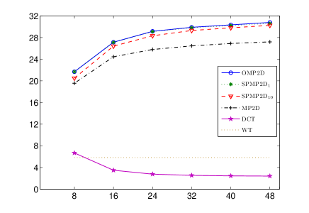
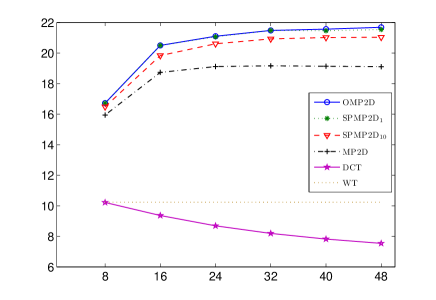
The points joined with different lines in the top left graph of Fig. 4 show results for the first image of Fig. 3 at the higher resolution ($4000\times 3552$ pixels). The results corresponding to the second image of Fig. 3, also at the higher resolution ($4000\times 4000$ pixels), are shown in the top right graph of Fig. 4. The bottom left and right graphs depict the same information as the top graphs but correspond to the screen size resolution of the images (size $1280\times 1574$ pixels and size $1280\times 1280$ pixels respectively).

Discussion of results

Let us start by highlighting the fact that the results of Fig. 4 illustrate a massive gain in sparsity yielded by the dictionary approach, in comparison to the DCT and DWT.

A clear feature in the results corresponding to the higher resolution images (top graphs of Fig. 4) is that, as opposed to the results for the DCT (decreasing curve in all the graphs of Fig. 4), the SR yielded by the dictionary approach increases with the block size, rapidly up to some value. For most images in the data set, and in particular for the two images of Fig. 3, block size $16\times 16$ yields the best trade off between sparsity and processing time (c.f. Tables 1).

The two bottom graphs confirm that, as should be expected, for the fixed PSNR of 45dB sparsity decreases with respect to the previous resolution and the block size has less relevance.

Notice that for the lower resolution image of the nebula, the SR shown in the bottom left graph of Fig. 4 becomes almost uniform for block sizes larger than $16\times 16$ pixels. For the lower resolution image of galaxy the SR shown in the bottom right graph of Fig. 4 increases with the block size, but much less than for the same image at higher resolution (top right graph).

Block size	OMP2D		SPMP2D1		SPMP2D10		MP2D
	SR	secs	SR	secs	SR	secs	SR	secs
$8\times 8$	21.69	51	21.69	61	20.52	60	19.55	56
$16\times 16$	27.63	98	27.61	115	26.41	99	24.49	93
$24\times 24$	29.15	233	29.08	209	28.28	200	25.79	205
$32\times 32$	29.97	506	29.88	392	29.30	382	26.46	387
$40\times 40$	30.36	1065	30.24	666	29.80	640	26.90	660
$48\times 48$	30.78	2041	30.60	1055	30.25	1015	27.20	1032
$8\times 8$	16.85	79	16.85	85	16.49	89	15.95	79
$16\times 16$	20.51	163	20.50	185	19.84	154	18.73	147
$24\times 24$	21.27	413	21.23	362	20.61	354	19.12	328
$32\times 32$	21.59	916	21.52	694	20.93	666	19.16	653
$40\times 40$	21.70	1989	21.59	1494	21.02	1145	19.13	1139
$48\times 48$	21.68	4031	21.53	2477	21.04	1919	19.11	1853

Table 1: SR and execution time, in secs, for approximating a complete image with different approaches and different sized blocks partitioning the image. The top half of the table corresponds to the results for the nebula at publication size resolution ($4000\times 3252$) pixels. The bottom half contains the results for the galaxy image at the equivalent resolution ($4000\times 4000$ pixels).

Table 1 compares the time (average of 5 independent runs) spent by the methods considered here, using the proposed dictionary, vs the size of the blocks partitioning the image. As can be observed, OMP2D implemented as described in Sec. 2.C is slightly faster than SPMP2D with projection step one, up to block size $24\times 24$, and becomes noticeable slower beyond that block size. This behavior is not a consequence of mathematical complexity, which as discussed in Sec 2.C in the best scenario are at most of the same order, but as a consequence of storage requirements. As the block size increases, the poor execution time scaling for OMP2D is a result of the additional memory required, over SPMP2D, for the storage of matrices $\mathbf{B}$ and $\mathbf{C}$ (c.f. (16)). Another interesting feature is that the results of SPMP2D with projection step larger than one do not improve the processing time significantly.

Experiment II

This experiment comprises a data set composed of fifty five images at screen size resolution, all of them in the category of nebulae, galaxies, and stars, taken from the top 100 images on the HST website [18]. Table 2 displays the average SR for the set, denoted as $\overline{{\mathrm{SR}}}$ as well as the average processing time, $\overline{t}$, per image in the set, using OMP2D, SPMP2D₁, SPMP2D₁₀, and MP2D, with partitions of square blocks of sides $8,16,24,32,$ and 40. The average size of the images in the set is $1264\times 1194$ pixels.

Block size	OMP2D		SPMP2D1		SPMP2D10		MP2D
	$\overline{{\mathrm{SR}}}$	$\overline{{\mathrm{t}}}$	$\overline{{\mathrm{SR}}}$	$\overline{{\mathrm{t}}}$	$\overline{{\mathrm{SR}}}$	$\overline{{\mathrm{t}}}$	$\overline{{\mathrm{SR}}}$	$\overline{{\mathrm{t}}}$
$8\times 8$	12.36	11.26	12.46	13.70	12.18	12.2	11.72	12.37
$16\times 16$	14.35	38.11	14.42	45.23	14.13	34.22	13.21	28.52
$24\times 24$	14.94	113.27	14.96	111.44	14.74	91.11	13.59	70.66
$32\times 32$	15.23	326.09	15.22	237.79	15.05	207.47	13.78	134.73
$40\times 40$	15.36	839.47	15.31	447.20	15.17	397.81	13.83	239.10

Table 2: Average SR ($\overline{{\mathrm{SR}}}$) and average processing time ($\overline{{\mathrm{t}}}$) per image (in secs) for approximating, up to a PSNR of 45 dB, a set of 55 images from the HST website. Both quantities are displayed against the block size partitioning the images. The average size of the images in the set is $1264\times 1194$ pixels. Note: the average times per image are also the average of 5 independent runs for each given block size.

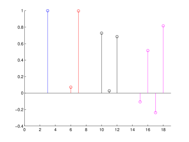
Now we are also interested in testing the proposed mixed dictionary against other possible mixed dictionaries. Preliminary experiments have shown that all combination of dictionaries containing a RDC (with redundancy two) component perform better than combinations without this component. Considering the preliminary tests we compare here the results obtained with the dictionaries of Sec. 2.B.1, against other mixed dictionaries containing a RDC component. The Euclidean basis is also included in all dictionaries. The comparison is carried out with respect to the remaining localized atoms. The RDBS dictionary is replaced by another one constructed in an equivalent manner using the prototypes in the top graphs of Fig. 5. The atoms of support 2,4,6, and 8, represented in the top right graph of Fig. 5, are discretized versions of Haar wavelets. The other prototypes are discretized versions of the continuous wavelets given in [31], the form of which is very similar to the Mexican Hat wavelet. Three fractional scaling parameters were used to produce discrete wavelets of support $3,5$, and $7$, represented in the top left graph of Fig. 5. We call this dictionary Redundant Discrete Wavelet (RDW) dictionary. For further comparison we constructed a random dictionary from normal distributed random atoms of support equal to the atoms of the dictionary we are testing against. We call such a dictionary Redundant Random (RR) dictionary. The prototypes corresponding to a particular realization of the random shapes are shown in the bottom graphs of Fig. 5.

Fig. 5: The two top graphs are the prototype atoms defining the RDW dictionary. The two bottom graphs are prototype atoms of random shape defining a realization of the RR dictionary.

For the experiment, five different realizations of a RR dictionary were tested. All the realizations produce similar results. The results displayed in Table 3 correspond to the average of the five realizations. Thus, the corresponding sparsity ratio ${\overline{\overline{{\mathrm{SR}}}}}$ is a double average. Namely, the average sparsity ratio $\overline{{\mathrm{SR}}}$ for the set of fifty five images and the average of this quantity ${\overline{\overline{{\mathrm{SR}}}}}$ with respect to the five realizations of the RR dictionary. As already mentioned the $\overline{{\mathrm{SR}}}$ does not depend significantly on the dictionary realization (the standard deviation of ${\overline{\overline{{\mathrm{SR}}}}}$ with respect to the five random realizations is, for all the block sizes, less than $4\%$ of the given ${\overline{\overline{{\mathrm{SR}}}}}$ values). The standard deviation with respect to the fifty five images is also the average $\overline{\sigma}_{\rm{SR}}$ corresponding to the five realization of the RR dictionary. Table  3 also shows the $\overline{{\mathrm{SR}}}$ and $\sigma_{\mathrm{SR}}$ for mixed dictionaries corresponding to the components RDBS and RDW and the corresponding standard deviations. All the dictionary results in Table 3 are obtained using the OMP2D method for block sides $8,16,24$ and $32$. The results from the DCT and DWT are also displayed.

Discussion of Results

This experiment confirms statistically the gain in sparsity obtained with the proposed dictionaries with respect to the DCT and DWT. It also confirms that the proposed approach SPMP2D₁ is a faster option for the implementation of OMP2D when the image partition is larger than $24$.

It is clear from Table 3 that, while the RDW and RR dictionary components produce comparable results, the differences with the RDBS component are significant, specially for the larger partition sizes. However, comparison with the $\overline{{\mathrm{SR}}}$ yielded by the DCT and DWT leads to the conclusion that it is the combination of a RDC dictionary with well localized atoms of arbitrary shape which yields a significant improvement in the sparsity of high quality approximations of astronomical images. Atoms of particular shape, such as the prototypes in the RDBS component improve sparsity even further.

Block size	RDCT-RDBS		RDCT-RDW		RDCT- RR		DCT		DWT
	$\overline{{\mathrm{SR}}}$	$\sigma_{\mathrm{SR}}$	$\overline{{\mathrm{SR}}}$	$\sigma_{\mathrm{SR}}$	${\overline{\overline{{\mathrm{SR}}}}}$	$\overline{\sigma}_{\rm{SR}}$	$\overline{{\mathrm{SR}}}$	$\sigma_{\mathrm{SR}}$	$\overline{{\mathrm{SR}}}$	$\sigma_{\mathrm{SR}}$
$8\times 8$	12.36	6.2	11.28	5.7	10.99	5.5	7.94	4.5	6.39	4.9
$16\times 16$	14.35	8.9	12.38	7.5	12.07	7.2	6.13	4.4	6.39	4.9
$24\times 24$	14.94	9.7	12.52	7.8	12.29	7.5	5.66	4.3	6.39	4.9
$32\times 32$	15.23	10.0	12.56	7.9	12.42	7.6	5.39	4.2	6.39	4.9

Table 3: Mean ($\overline{{\mathrm{SR}}}$) and variance ($\sigma_{\mathrm{SR}}$) of the SR obtained with different mixed dictionaries, by partitioning the images into blocks of size 8, 16, 24 and 32 and applying the OMP2D approach with RDCT-RDBS, RDCT-RDW and RDCT-RR dictionaries. The results from the approximation with the transforms DCT and WT are also shown.

4 Conclusions

Sparse representation of astronomical images has been considered. A mixed dictionary composed of a RDC component and a RDBS component was proposed. Using a data set of fifty five astronomical images in the category of nebulae, galaxies, and stars, the dictionary was shown to be suitable for sparse representation of that class of images. From the experiments involving atoms of different shapes one can assert that the combination of a RDC component with a component of localized atoms of different support yields the most important gain in sparsity, with respect to results from the popular transforms DCT and DWT. Nevertheless, the proposed particular shape of the RDBS component represents an advantage over other possible atoms of equal support, and yields an impressive sparsity gain over DCT and DWT results.

The fact that the proposed dictionary is suitable for block processing by the selection technique OMP2D makes the resulting approach very effective in terms of processing time. For the data set characterized by an average sparsity ratio of $12.6$ (with standard deviation $6.2$) the processing time, for partition size $8\times 8$, is only $11.26$ secs per image of average size of $1264\times 1194$ pixels. This should be appreciated taking into account that the time refers to executing a C++ MEX file in a MATLAB environment, using a small laptop with the specification details given in Sec. 3.

Specially for high resolution images, sparsity may significantly increase with the partition size. In order to handle these cases, a greedy strategy taking full advantage of the separability property of the proposed dictionaries was considered. The approach has been termed SPMP2D, because it allows to orthogonalize the seminal MP technique by self-projections. Through the experiments the technique was established as a convenient alternative to OMP2D, when the latter scale badly due to storage demands, or the storage capacity is not available.

Finally we would like to highlight that, even though for small partitions the approach is fast for sequential computing, the possibility of its parallel implementation is only a question of resource availability. The approach obeys a scaling law by independently processing the blocks partitioning the image. Hence, a straightforward multiprocessor implementation would reduce the processing time of the sequential implementation by a factor approximatelly equal to the number of processors.

The results presented in this Communication are truly encouraging and we feel confident that the approach will benefit applications relying on sparse representation of digital images.

Acknowledgements

Support from EPSRC, UK, grant (EP$/$D062632$/$1) is acknowledged. The MATLAB files and C++ MEX files for implantation of the OMP2D and SPMP2D methods are available at [29]. We are grateful to ESO and HST for making publicly available the images that have been used for the experiments.

References

- [1] S. Fischer, G. Cristóbal, R. Redondo, “Sparse overcomplete Gabor wavelet representation based on local competitions” IEEE Transactions on Image Processing 15, 265 – 271 (2006).
- [2] J. Mairal, M. Eldar, G. Sapiro, “Sparse Representation for Color Image Restoration”, IEEE Transactions on Image Processing 17, 53 – 69 (2008).
- [3] L. P. Yaroslavsky, G. Shabat, B. G. Salomon, I. A. Ideses, and B. Fishbain, “Nonuniform sampling, image recovery from sparse data and the discrete sampling theorem”, J. Opt. Soc. Am. A 26, 566–575 (2009).
- [4] J. Wright, Yi Ma, J. Mairal, G. Sapiro, T.S. Huang, and S. Yan, “Sparse Representation for Computer Vision and Pattern Recognition”, Proceedings of the IEEE 98, 1031 – 1044 (2010).
- [5] J-L. Starck, F. Murtagh and J. M. Fadili, “Sparse Image and Signal Processing”, Cambridge University Press, 2010.
- [6] E. Candès and M. Wakin, “An introduction to compressive sampling”, IEEE Signal Processing Magazin 25, 21 – 30 (2008).
- [7] J. Romberg, “Imaging via compressive sampling”, IEEE Signal Processing Magazine 25, 14 – 20 (2008).
- [8] R. Baraniuk, “More Is less: Signal processing and the data deluge”, Science 331, 717 – 719 (2011).
- [9] Z. Xu and E. Y. Lam, “Image reconstruction using spectroscopic and hyperspectral information for compressive terahertz imaging”, J. Opt. Soc. Am. A 27, 1638–1646 (2010).
- [10] A. Fannjiang and H-C Tseng, “Compressive imaging of subwavelength structures: periodic rough surfaces”, J. Opt. Soc. Am. A 29, 617–626 (2012).
- [11] J. Bobin, J-L. Stack and R. Ottensamer, “Compressed sensing in astronomy”, IEEE Journal of Selected Topics in Signal Processing 2, 718 –726 (2008).
- [12] J-L. Stack and J. Bobin, “Astronomical data analysis and sparsity: from wavelets to compressed sensing,” Proceeding of the IEEE 98, 1021–1030 (2009).
- [13] H. Rauhut, K. Schnass and P. Vandergheynst, “Compressed sensing and redundant dictionaries”, IEEE Trans. on Information Theory, 54, 2210–2219 (2008).
- [14] E. Candès, Y. Eldar, D. Needell and P. Randall, “Compressed sensing with coherent and redundant dictionaries,” Applied and Computational Harmonic Analysis, 31, 59–73 (2011).
- [15] J. Bowley and L. Rebollo-Neira, “Sparsity and something else: an approach to encrypted image folding” IEEE Signal Processing Letters, 8, 189–192 (2011).
- [16] L. Rebollo-Neira, J. Bowley, A. Constantinides and A. Plastino, “Self contained encrypted image folding”, Physica A 391, 5858–5870 (2012).
- [17] http://http://www.eso.org/public/
- [18] http://hubblesite.org/
- [19] R. Young, “An Introduction to Nonharmonic Fourier Series”, Academic Press, New York, 1980.
- [20] S.S. Chen, D.L. Donoho, and M.A. Saunders. Atomic decomposition by basis pursuit. SIAM Journal on Scientific Computing 20, 33–61 (1998).
- [21] S. G. Mallat and Z. Zhang, “Matching Pursuits with Time-Frequency Dictionaries”, IEEE Transactions on Signal Processing 41, 3397–3415 (1993).
- [22] L. K. Jones, “On a Conjecture of Huber Concerning the Convergence of Projection Pursuit Regression”, Ann. Statist. 15, 880–882 (1987).
- [23] Y.C. Pati, R. Rezaiifar, and P.S. Krishnaprasad, “Orthogonal matching pursuit: recursive function approximation with applications to wavelet decomposition,” Proceedings of the 27th Annual Asilomar Conference in Signals, System and Computers, vol 1, pp 40–44, (1993).
- [24] L. Rebollo-Neira and D. Lowe, “Optimized orthogonal matching pursuit approach”, IEEE Signal Processing Letters 9, 37–140 (2002).
- [25] M. Andrle and L. Rebollo-Neira, “A swapping-based refinement of orthogonal matching pursuit strategies,” Signal Processing 86, 480–495 (2006).
- [26] M. Andrle and L. Rebollo-Neira, “Cardinal B-spline dictionaries on a compact interval,” Applied and Computational Harmonic Analysis 18, 336–346 (2005).
- [27] L. Rebollo-Neira and Z. Xu, “Adaptive non-uniform B-spline dictionaries on a compact interval”, Signal Processing, doi:10.1016j.sigpro.2010.02.004, 2010.
- [28] C. de Boor A Practical Guide to Splines Applied Mathematical Sciences, vol. 27, Springer-Verlag, New York (1978).
-
[29]
Highly nonlinear approximations for sparse signal representation.
http://www.nonlinear-approx/info. - [30] Z. Wang, A. C. Bovik, H. R. Sheikh, E. P. Simoncelli, Image quality assessment: “From error visibility to structural similarity”, IEEE Transactions on Image Processing, 13 (2004) 600–612 (2004).
- [31] I. Daubechies, Ten Lectures on Wavelets, Society for Industrial and Applied Mathematics, 1992.