Comparative Modelling of the Spectra of Cool Giants^,

Abstract

Context. Our ability to extract information from the spectra of stars depends on reliable models of stellar atmospheres and appropriate techniques for spectral synthesis. Various model codes and strategies for the analysis of stellar spectra are available today.

Aims. We aim to compare the results of deriving stellar parameters using different atmosphere models and different analysis strategies. The focus is set on high-resolution spectroscopy of cool giant stars.

Methods. Spectra representing four cool giant stars were made available to various groups and individuals working in the area of spectral synthesis, asking them to derive stellar parameters from the data provided. The results were discussed at a workshop in Vienna in 2010. Most of the major codes currently used in the astronomical community for analyses of stellar spectra were included in this experiment.

Results. We present the results from the different groups, as well as an additional experiment comparing the synthetic spectra produced by various codes for a given set of stellar parameters. Similarities and differences of the results are discussed.

Conclusions. Several valid approaches to analyze a given spectrum of a star result in quite a wide range of solutions. The main causes for the differences in parameters derived by different groups seem to lie in the physical input data and in the details of the analysis method. This clearly shows how far from a definitive abundance analysis we still are.

1 Introduction

Spectroscopy is the basic tool of modern astrophysics. It is the key for revealing the elemental composition and the physical conditions in the spectrum-forming layers of stars. Interpreting the information contained in the spectra requires knowledge about the physics of the stellar atmosphere, the line formation processes, and the atomic and molecular data. Parameters derived from the analysis of high-resolution spectra via comparison with stellar models have great potential but suffer from systematic uncertainties due to insufficient input physics in both the model atmospheres and the spectral synthesis, as well as to different fitting approaches.

Several codes to calculate atmospheric models exist today and are used by various groups around the world to analyze both spectroscopic and photometric data. However, the implementation of the physics, the atomic and molecular data used, and the details of the method of deriving stellar parameters from the observed data differ among the various research groups. Therefore, a comparison of the various codes and their output may help us understand uncertainties in the analysis of stellar spectra introduced by these various components involved in the fitting process. These uncertainties also have a major impact on the interpretation of photometric data or the modelling of stellar populations.

In this paper we present a comparison of a variety of model codes that attempt to analyze the spectra of cool giants. Red giant stars are quite challenging targets for modelling with their complex atmospheres and the large number of lines, in particular those of molecular origin. Hence, they provide a good testbed for exploring the validity of input physics, line data, and modelling approaches. The aim was to test how comparable the results are when applying different methods.

For this comparison, three of us (U. Heiter, T. Lebzelter, W. Nowotny) designed the following experiment, hereafter referred to as Experiment 1: colleagues, who are engaged in stellar parameter and abundance determinations for cool giants on a regular basis, received high resolution and high signal-to-noise ratio (S/N) spectra of four cool stars and were asked to derive their fundamental stellar parameters, such as the effective temperature ($T_{\rm eff}$), the surface gravity ($\log g$), and the metallicity ([Fe/H]). In addition, we provided corresponding photometric data in various bands. However, no identifications of the sources were given in order to prevent the participants from comparing their findings with data in the literature. The list of authors of this paper illustrates the high level of interest in this experiment. The results were compared and discussed during a workshop held at the University of Vienna, August 23-24, 2010.

The choice of cool giants as targets was driven by the motivation of this experiment within the framework of ESA’s upcoming Gaia mission. In preparation for the exploitation of a large amount of spectroscopic and photometric data with the aim of determining accurate stellar parameters, there is a clear need to identify key areas where model spectra can and should be improved, and to determine the influence of different methods of analysis on the results. Giant stars will play an important role within the sample of objects that will be studied by Gaia.

At the workshop we agreed to perform a second comparison of our models, hereafter referred to as Experiment 2. In this case, each participating group was asked to calculate a high-resolution model spectrum in a pre-defined wavelength range using a given set of stellar parameters.

This article is organized as follows. In Section 2 we provide details on the design of the experiments, and summarize the properties of the two benchmark stars analysed in Experiment 1, $\alpha$ Tau and $\alpha$ Cet. A detailed description of the modelling approaches used in the experiments is presented in Section 3. In Sections 4 and 5 the results of both experiments are presented and discussed. As a by-product we give revised stellar parameters for the two benchmark stars. The outcome of our experiments forms a basis for future improvements of stellar spectrum modelling. This will be an important step towards accurate stellar parameters of giant stars observed by Gaia and Gaia follow-up programmes.

2 Experiment set-up and benchmark stars

2.1 Experiment 1 – stellar parameter determination

High-resolution and high S/N spectra of four targets were provided for Experiment 1. Two of them were of real stars, namely $\alpha$ Tau and $\alpha$ Cet, and covered the visual range of the spectrum between 4900 and 9750 Å. They were obtained by one of us (U. Heiter) using the NARVAL spectrograph at the 2m Telescope Bernard Lyot atop Pic du Midi (Aurière 2003). The resolution was set to $R$=80 000. S/N$>$200 was achieved throughout the whole spectral range for both stars. The data were reduced with the Libre-ESpRIT pipeline (Donati et al. 1997). The extracted and calibrated echelle orders were merged by cutting the orders at the centers of the overlap regions. The spectra were not corrected for telluric features, but a spectrum of a telluric standard star taken in the same night was provided. Both objects have been studied in detail in the past and have been used as reference targets in several investigations. In Table 1 we summarize the stellar parameters which we assume are the most accurate ones available in the literature. A more detailed description of the targets is given in Sections 2.2 and 2.3. Three wavelength ranges were recommended, on which the experiment should focus: $[4900-5400]$, $[6100-6800]$ and $[8400-8900]$ Å. Only the second of these regions was judged to be significantly contaminated by telluric lines.

The other two spectra were synthetic ones computed for realistic stellar parameters. Within the experiment they should allow for a more direct comparison between the models without the uncertainties of stellar parameters and the unidentified features we see in observed data. For the artificial data we used two COMARCS model spectra (for a description of the COMARCS models see Sect. 3.1.1) calculated by W. Nowotny and T. Lebzelter. To simulate observational effects some gaussian noise was added (S/N=125) and the output was rebinned from $R$=300 000 to $R$=50 000. The chosen model parameters are listed in Table 2. The input parameters for Star 3 were chosen to reproduce a slightly metal poor K-type giant as might be found in an Large Magellanic Cloud cluster. Star 4 should resemble a typical field star on the Asymptotic Giant Branch (AGB). The corresponding quantities follow the predictions from the stellar evolution models by Marigo et al. (2008). The ratio of ¹²C to ¹³C was solar in both cases. For the synthetic spectra we chose a wavelength range of $\lambda=$15 456–15 674 Å. Within this part of the spectrum one finds lines of CO, OH and CN as well as several atomic lines. The wavelength range is almost free of telluric lines (e.g. Hinkle et al. 1995). The synthetic spectra have a much smaller wavelength coverage than the NARVAL spectra which reflects the fact that today’s near infrared spectrographs that reach a resolution of $R$=50 000 (CRIRES, Phoenix) also cover only a comparably small wavelength range at a time. Broad band colours of the model stars, listed in Table 2 as well, have been calculated from lower resolution spectra ($R$=10 000) over a wavelength range from 0.45 to 2.6 $\mu$m as described in Nowotny et al. (2011). The participants of the experiment were not informed about the artificiality of these data. All four spectra used in Experiment 1 are available online.

A specific list of atomic line data was provided, and was suggested, but not required, to be used for the analysis. This line list was extracted on 2010-04-29 from the Vienna Atomic Line Database (VALD) (Uppsala mirror; Piskunov et al. 1995; Kupka et al. 1999; Heiter et al. 2008), and included all lines in the database within the three recommended optical wavelength regions and the single infrared region.

Table 1: Stellar parameters of $\alpha$ Tau (Section 2.2) and $\alpha$ Cet (Section 2.3) based on published data.

	$\alpha$ Tau	Ref.	$\alpha$ Cet	Ref.
	Star 1		Star 2
Name	Aldebaran		Menkar
HR	1457		911
MK type	K5 III		M1.5 IIIa
$T_{\rm eff}$ (K)	3930$\pm$40	(a)	3800$\pm$60	(a)
$T_{\rm eff}$ (K)	3920$\pm$130	(b)	3730$\pm$75	(i)
$L$ [$L_{\odot}$]	440$\pm$20	(c)	1870$\pm$130	(c)
log ($g$ (cm s-2))	1.2$\pm$0.1	(a)	0.9$\pm$0.1	(a)
log ($g$ (cm s-2))	1.2$\pm$0.5	(b)	0.7$\pm$0.3	(i)
$M$ [$M_{\odot}$]	1.3$\pm$0.3	(d)	3.0$\pm$0.5	(d)
$[$Fe/H$]$	$-$0.22$\pm$0.11	(e)	+0.02$\pm$0.03	(i)
$V-I$	2.17$\pm$0.02	(f)	2.51$\pm$0.02	(f)
$J-K$	0.97$\pm$0.03	(f)	1.08$\pm$0.03	(f)
$V-K$	3.67$\pm$0.03	(f)	4.21$\pm$0.03	(f)
$v_{\rm rad}$ [km s-1]	54.26$\pm$0.03	(g)	$-$26.08$\pm$0.02	(g)
$v$ sin $i$ [km s-1]	5$\pm$1	(h)	3$\pm$2	(j)

Table 2: Input parameters and model colours for the two artificial stars in Experiment 1.

	Star 3	Star 4
$T_{\rm eff}$ (K)	4257	3280
$L$ [$L_{\odot}$]	319	3816
log ($g$ (cm s-2))	1.47	0.06
$M$ [$M_{\odot}$]	1.165	1.509
$[$Fe/H$]$	$-$0.4	+0.1
C/O	0.35	0.55
$V-I$	1.25	3.58
$J-K$	0.82	1.23
$V-K$	2.94	6.89

2.2 $\alpha$ Tau

Stellar surface parameters ($T_{\rm eff}$ and $\log g$) can be determined either from angular diameter measurements in combination with additional data (called direct parameters hereafter), or from a model atmosphere analysis of photometric or spectroscopic data. The direct $T_{\rm eff}$ value is obtained from the angular diameter $\theta$ and the bolometric flux $F_{\rm bol}$ according to Eq. 1, where $\sigma$ is the Stefan-Boltzmann constant. The direct $\log g$ value is derived from $\theta$, the stellar mass $M$, and the parallax $\pi$ according to Eq. 2, where $R$ is the linear stellar radius and $G$ is the constant of gravity.

$$T_{\rm eff}^{4}=\frac{F_{\rm bol}}{\sigma(0.5\theta)^{2}}$$ (1)

$$g=\frac{GM}{R^{2}};\,R=\frac{\theta}{2\pi}$$ (2)

The angular diameter of $\alpha$ Tau was determined recently by Richichi & Roccatagliata (2005), using both lunar occultations and long-baseline interferometry (VLTI-VINCI, $K$-band), and taking into account limb darkening. The integrated absolute flux was measured for $\alpha$ Tau by di Benedetto & Rabbia (1987) and Mozurkewich et al. (2003). The measured $\theta=20.58\pm 0.03$ mas and $F_{\rm bol}=33.57\pm 1.35$ nW m^-2 result in the direct $T_{\rm eff}$ value given in Table 1. With the Hipparcos parallax $\pi=48.92\pm 0.77$ mas (van Leeuwen 2007), this results in $R=45.2\pm 0.7\leavevmode\nobreak\ R_{\odot}$ and in the luminosity $L$ given in Table 1. We estimate the mass of $\alpha$ Tau using two different sets of stellar evolutionary tracks, those published by the Padova group (Bertelli et al. 2008, 2009) and the Yonsei-Yale (Y2) models (Yi et al. 2003; Demarque et al. 2004). For solar metallicity tracks (Padova: $Z$=0.017, $Y$=0.26; Y2: $Z$=0.02, $X$=0.71), the direct $T_{\rm eff}$ and $L$ imply a mass of 1.6$M_{\odot}$ for both model grids, while the metal-poor tracks corresponding to [Fe/H]=$-$0.3 (Padova: $Z$=0.008, $Y$=0.26; Y2: $Z$=0.01, $X$=0.74) suggest a mass of 1.0 to 1.1 $M_{\odot}$. Interpolating between these values results in the mass in Table 1. Thus, we arrive at the $\log g$ value for $\alpha$ Tau given in Table 1.

$\alpha$ Tau has been studied with high resolution, high S/N spectra in nine publications since 1980 (according to the PASTEL catalogue, Soubiran et al. 2010). The stellar parameters derived in these works and the references are given in Table 3. Effective temperatures used in the spectroscopic analyses have been derived from various photometric calibrations by most authors. Combining the results given in six publications, the mean published photometric $T_{\rm eff}$ of $\alpha$ Tau is 3850$\pm$40 K. This is in good agreement with the latest value of $T_{\rm eff}$=3880$\pm$40 K determined with the infrared flux method (IRFM), by Ramírez & Meléndez (2005), which is an update of the work by Alonso et al. (1999). Two publications from 1981 and 2007 derive $T_{\rm eff}$ in a spectroscopic way (excitation equilibrium of iron line abundances) from high-resolution spectra in the optical wavelength range. They arrive at almost the same value, close to 4120 K, which is significantly higher than the photometric one. On the other hand, Meléndez et al. (2008) obtained a spectroscopic $T_{\rm eff}$ of 3890 K, close to the IRFM value, based on high-resolution infrared spectra centered on 15555 Å.

The method for determining the surface gravity varies significantly between the publications. Four of the authors derive $\log g$ in a spectroscopic way in the optical wavelength range (ionization equilibrium of iron line abundances) and arrive at a mean value of 1.1$\pm$0.5. Two authors use absolute magnitudes and stellar evolution calculations, and cite a higher mean value of 1.6$\pm$0.1. The spectroscopic $\log g$ of Meléndez et al. (2008) determined from IR spectra is close to the values obtained from optical spectra. The highest $\log g$ value of 1.8 is determined from DDO photometry by Fernandez-Villacanas et al. (1990), who cite an error of 0.2.

The metallicity of $\alpha$ Tau is determined in eight publications and found to be below solar (mean value $-0.2\pm 0.1$, see Table 1). The results can be divided into two groups, three authors using $T_{\rm eff}$$>$3900 K and five authors using $T_{\rm eff}$$<$3900 K. The corresponding [Fe/H] values cluster within a few tenths of a dex around $-0.35$ and $-0.15$, respectively. The mean $T_{\rm eff}$ and $\log g$ values used for deriving the mean [Fe/H] are given in Table 1.

The spectral type K5 III given for $\alpha$ Tau in Table 1 was first published in the original MKK Atlas (Morgan et al. 1943) and has been quoted throughout the literature. However, the star’s TiO strength, as measured by narrow-band classification photometry (Wing 2011), yields a spectral type of K5.7 III on a scale where type M0.0 immediately follows K5.9. The photometric colours also indicate an effective temperature closer to M0.0 than to K5.0.

Table 3: Results and references for previous spectroscopic works on $\alpha$ Tau.

$T_{\rm eff}$	(a)	$\log g$	(b)	[Fe/H]	Reference
4140	sp	1.0	sp	$-$0.33	Lambert & Ries (1981)
3830	ph	1.2	sp	$-$0.14	Kovacs (1983)
3850	ph	1.5	ev	(c)	Smith & Lambert (1985)
3800	ph	1.8	ph	$-$0.17	Fernandez-Villacanas et al. (1990)
3910	ph	1.6	ev	$-$0.34	McWilliam (1990)
3875	ph	0.6	sp	$-$0.16	Luck & Challener (1995)
3850	ph	0.6	li	$-$0.10	Mallik (1998)
4100	sp	1.7	sp	$-$0.36	Hekker & Meléndez (2007)
3890	sp	1.2	sp	$-$0.15	Meléndez et al. (2008)

2.3 $\alpha$ Cet

The angular diameter of $\alpha$ Cet was determined by Wittkowski et al. (2006a) from long-baseline interferometry, using the same instrumentation as for $\alpha$ Tau, and taking into account limb darkening. The same authors also determined $F_{\rm bol}$ from integrated absolute flux measurements. The measured $\theta=12.20\pm 0.04$ mas and $F_{\rm bol}=10.3\pm 0.7$ nW m^-2 result in the direct $T_{\rm eff}$ value given in Table 1. With the Hipparcos parallax $\pi=13.10\pm 0.44$ mas (van Leeuwen 2007), this results in $R=100\pm 3\leavevmode\nobreak\ R_{\odot}$ and in the luminosity $L$ given in Table 1. Using this luminosity and the direct $T_{\rm eff}$ value, we estimate the mass of $\alpha$ Cet (see Table 1) from evolutionary tracks for solar metallicity (see Section 2.2). The masses from the two different sets of models agree within 0.1 $M_{\odot}$ The 2007 Hipparcos parallax is smaller than the “original” one by about 10%, which results in a mass 30% higher than derived by Wittkowski et al. (2006a). The mass estimate could be refined in the future through asteroseimology, but in any case the uncertainties for the direct $\log g$ value are already much smaller than the spectroscopic uncertainties. As for $\alpha$ Tau, from these stellar data we can derive an accurate direct $\log g$ value for $\alpha$ Cet, given in Table 1.

For $\alpha$ Cet, there are no previously published high-resolution spectroscopic studies in the optical wavelength range. The $T_{\rm eff}$ value determined with the IRFM value is 3720$\pm$50 K (Ramírez & Meléndez 2005). The star is included in the infrared spectroscopic study of Meléndez et al. (2008), who determine a spectroscopic $T_{\rm eff}$ close to the IRFM value, a spectroscopic $\log g$= 0.7$\pm$0.3, and solar metallicity (see Table 1). The TiO-based spectral type of $\alpha$ Cet, from narrow-band classification photometry (Wing 2011), is M1.7 III, in substantial agreement with the Morgan-Keenan (MK) type shown in Table 1.

2.4 Experiment 2 – comparison of synthetic spectra for fixed parameters

For this experiment the set of stellar parameters was predefined in order to be able to compare the output of the various combinations of models and spectral synthesis codes directly. Participants were asked to compute spectra at high resolution ($R\geq$ 300 000) for $T_{\rm eff}=$3900 K, $\log g$= 1.3, and [Fe/H]$=-0.2$, i.e. a parameter set close to the values corresponding to $\alpha$ Tau. Microturbulence was fixed at 2.0 km s^-1, and a mass of 2 $M_{\odot}$ was to be assumed. The synthetic spectra covered the three optical wavelength regions that were recommended for the analysis of Star 1 and Star 2 in Experiment 1. The same abundance pattern (Asplund et al. 2009) was used by all participating groups.

3 Modelling

In this section we summarize the main characteristics of the models used for the experiments. In our sample we have two major model ‘families’ – MARCS (Model Atmospheres in a Radiative Convective Scheme) and ATLAS – where several implementations and individual further developments of the original code were employed, and three alternative models. For the discussion below we introduce abbreviations for each model and implementation, e.g. ‘M’ for MARCS-based modelling, and ‘M1’ for a specific participating team applying the code. Where possible we refer to more extensive descriptions of the codes published elsewhere. Comparisons of different atmospheric models can be found in the original literature describing the codes. For example, Gustafsson et al. (2008) write on the comparison between MARCS and ATLAS models:

“In view of the fact that these two grids of models are made with two totally independent numerical methods and computer codes, with independent choices of basic data (although Kurucz’s extensive lists of atomic line transitions are key data underlying both grids), this overall agreement is both satisfactory and gratifying.”

Figure 1: Wavelength intervals used by the eleven different groups analysing the optical spectra. See §§ 3.1 to 3.5. For the M3b analysis (§ 3.1.3), discontinuous wavelength regions totaling $\sim$435Å were used. The M6, A1, and A4 groups (§§ 3.1.6, 3.2.1, and 3.2.4) used spectrum synthesis for individual spectral lines distributed over the indicated regions. The A2 and A5 groups (§§ 3.2.2, and 3.2.5) used equivalent widths for individual spectral lines.

Each group worked with different subsections of the available wavelength range. For the optical spectra, Fig. 1 shows the wavelength intervals used by the eleven groups who analyzed these spectra. Most groups analysing the spectra of Star 1 and Star 2 determined radial velocities, which are given in Tables 12 and 13, and corrected the observed spectra to laboratory wavelengths. The groups used different approaches to adjust the continuum scale of these spectra, which are described in the individual subsections.

The groups employing MARCS model atmospheres in general used the solar chemical composition from Grevesse et al. (2007) as a reference (which was used for the calculation of the on-line database of MARCS models). However, M1 (Section 3.1.1) adopted the abundances from Grevesse & Sauval (1994) for C, N, and O, and from Anders & Grevesse (1989) for all other elements. A3 used only the latter source for their reference abundance pattern. A4 (Section 3.2.4) took their reference abundance pattern from Grevesse & Sauval (1998). The analysis of A5 (Section 3.1.5) refers to the abundances of Asplund et al. (2005). M5, A1, and A2 (Sections 3.1.5, 3.2.1, and 3.2.2) used the solar abundances from Asplund et al. (2009), and P and C (Sections 3.3 and 3.4) those of Grevesse et al. (1996). T used abundance values from several sources summarized in Table 4, case (b), of Tsuji (2008), and in Tsuji (2002).

Table 4: Overview of model grid parameters used by different groups in Experiment 1.

ID	$T_{\rm eff}$	$\log g$	[Fe/H]
	(K)	(cm s-2)
M1	3600 to 4000 / 50	0.5, 1.0, 1.5	0.0, $-$0.3, $-$0.5
M2	3500 to 4100 / 100	0.5 to 2.0 / 0.5	$-$0.5 to +0.5 / 0.25
M3	2500 to 8000	0.0 to 5.0	$-$5.0 to +1.0
M4	3800 to 4300 / 50	0.0 to 3.0 / 0.5	0.0, $-$0.25
M5	2500 to 8000 / 250	$-$1 to 5 / 0.5	$-$5 to 1 /
M6	3750 to 4250 / 200	0.0 to 2.0 / 1.0	-1.0 to 0.5 / 0.1
A1	3500 to 13000 / 250	0.0 to 5.0 / 0.5	$-$1.5 to +0.5 / 0.5
A2	3500 to 6000 / 250	0.0 to 5.0 / 0.5	$-$1.5 to +0.5 / 0.5
A3	3000 to 8000 / 100	0.0 to 3.0 / 0.1	0.0
A4	3500 to 6250 / 250	0.0 to 5.0 / 0.5	+0.5, +0.2, +0.0;
			$-$0.5 to $-$4.5 / 0.5
A5	3500 to 6000 / 250	0.0 to 5.0 / 0.5	0.0, -1.0
P	3500 to 4500 / 125	1.0 to 2.5 / 0.5	0.0, $-$0.5
T	2800 to 4000 / 100	$-$0.52 to 1.34 /	0.0
C	2600 to 4000 / 200	$-$0.5, 0.0	$-$0.5, 0.0

Some of the groups determined stellar parameters from the photometric colours provided together with the spectra for each star. These parameters, and the corresponding photometric calibrations, are summarized in Tables 12 to 15. Table 4 summarizes the range of parameters of the model grids used by several of the groups for the determination of the best-fit spectrum.

Sections 3.1 to 3.5 contain detailed accounts of the analysis work of the participating groups. In these sections, Star 1 and Star 2 refer to $\alpha$ Tau and $\alpha$ Cet, respectively. Each modelling description also includes a brief discussion of the individual fitting results. The impatient reader may at this point skip to Section 4, where we start with an overview of the main aspects of each analysis, and the detailed descriptions may serve for later reference. A general discussion comparing the results from the various groups is provided in Section 5.

3.1 MARCS model atmospheres (M)

3.1.1 M1

The Padova-Vienna team included B. Aringer, T. Lebzelter, and W. Nowotny. This analysis used the COMARCS hydrostatic atmosphere models, which are a further development of the original MARCS code of Gustafsson et al. (1975) and Jørgensen et al. (1992). Opacities are treated using opacity tables created in advance with the opacity generation code coma08 (Aringer et al. 2009). Compared to the MARCS models of Gustafsson et al. (2008), the opacities are computed with different interpolation schemes. The temperature and, accordingly, the pressure stratification of the models are derived under the assumption of a spherical configuration in hydrostatic and local thermodynamic equilibrium (LTE). A detailed description of the spectral synthesis is given in Nowotny et al. (2010). Sources for spectral line data are given in Lederer & Aringer (2009).

Recent applications to the fitting of observed high-resolution spectra can be found in Lebzelter et al. (2008) and Lederer et al. (2009). Here the same approach of finding the best fit was used, which will be briefly sketched in the following. Note that only the two spectra in the visual range, Star 1 and Star 2  were fitted. The same codes were used to calculate the two artificial sample spectra, Star 3 and Star 4 , and the corresponding broad band photometry.

The M1 analysis started by calculating a grid of model spectra (see Table 4) at $R$=300 000, rebinned to $R$=80 000 afterwards. Broad band model colours were determined, too, following descriptions in Nowotny et al. (2011). Microturbulence and macroturbulence were set to fixed values (see Tables 12 and 13). The value for the macroturbulence was checked with the typical line widths in the observed spectrum, and was found to be reasonably chosen.

The first step was to identify features in the optical range that are primarily sensitive to changes of a single stellar parameter. The starting point for finding the best fit was the calcium triplet which constrained the value for $\log g$. This estimate was validated by checking a few obviously $\log g$ sensitive lines between 8500 and 8800 Å. Because the strength of these lines is also dependent on the metallicity, it was decided to determine the best fitting $\log g$ value for all three [Fe/H] values of the grid independently. Next, the temperature was fixed based on the strength of the TiO band heads at 6652, 6681, and 6698 Å. The temperature was derived for each of the three metallicity / $\log g$ pairs from the previous step. A semiempirical approach combining $\chi^{2}$ analysis with a check of the fit by eye was applied. In cases where the best fit seemed to fall between two points of the model grid, the final fit parameters were determined by interpolation between these grid points. For Star 1  this resulted in the best fitting parameter combinations ($T_{\rm eff}$, $\log g$, [Fe/H]) = (3900 K, 1.25, 0.0), (3800 K, 0.75, $-$0.3), and (3750 K, 0.5, $-0.5$). For Star 2, the corresponding values are (3800 K, 1.0, 0.0), (3700 K, 0.5, $-$0.3), and (3675 K, 0.5, $-$0.5).

The best combination of metallicity, temperature and $\log g$ should then be determined by testing the overall fit of the atomic lines and molecular bands at shorter wavelengths. However, no clear decision could be made in that respect, either for Star 1 or for Star 2. It turned out that the fit of the spectrum below 6000 Å became rather poor with several missing lines. Furthermore, several lines came out too strong from the model, and it is suspected that incorrect line blends are responsible for this problem. Tentatively, an [Fe/H] value below solar seems to be more appropriate for both stars.

To further constrain the metallicity of the star, synthetic colours for the chosen best fit combinations were compared with the observed values. For Star 1, the three given colours (see Table 1) are best represented by the solution for [Fe/H] = $-0.3$. For Star 2, the solution for [Fe/H] = $-0.5$ fits best, and the solar abundance model can be excluded. These solutions are given in Tables 12 and 13 (see §4 below). The error bars are derived from the different metallicities considered.

3.1.2 M2

In the M2 analysis, Star 1 and Star 2 were studied by B. Plez. Spectra were computed using the TURBOSPECTRUM code (Alvarez & Plez 1998). Model atmospheres were extracted from the MARCS database (Gustafsson et al. 2008). Refinement in the grid of models was obtained by interpolation using the routines by Masseron (2006), provided on the MARCS site. Molecular line lists are described in Gustafsson et al. (2008), and atomic lines were extracted from the VALD database. As in the MARCS calculations, collisional line broadening is treated following Barklem et al. (2000), with particular broadening coefficients for many lines.

The comparison between observations and calculations was done using a mean square differences computation. As a first step, the photometry provided with the data was used to derive a first estimate of $T_{\rm eff}$. Colour – $T_{\rm eff}$ calibrations based on MARCS models were used (Bessell et al. 1998; van Eck et al. 2011). Spectra were then computed for spherical models of one solar mass, with $T_{\rm eff}$ $\pm$200 K around these values, gravities typical for giants, a range of metallicities, and fixed values for the microturbulence parameter (see Table 4). The differences between observed ($o_{i}$) and calculated ($c_{i}$) spectra with $N$ wavelength points were characterized by $\sigma=\sum_{i=1}^{N}\frac{(o_{i}-c_{i})^{2}}{N}$ computed for wide portions of the spectra (see Fig. 1).

This computation quickly showed that models with different parameter combinations (e.g. a lower $T_{\rm eff}$ and a lower metallicity) could give similarly small values of $\sigma$. Also, different spectral regions would lead to best fits for different values of the stellar parameters. The reason is that the spectra are dominated by numerous atomic and molecular lines, for which the line position and strength data might not be sufficiently accurate. The result is then that many small differences add up to a relatively large $\sigma$ that becomes quite insensitive to local improvements on a few “good” lines. Another problem is caused by the normalization of the observed spectra, which leaves residual slopes relative to the calculations. This is especially problematic for spectra of cooler objects with many molecular bands. Robust methods indeed use only the information from selected spectral ranges, where line data are carefully calibrated, and where spectra can be renormalized easily. This selection was not done owing to the limitations of present experiment.

Values of $\sigma$ were also computed for a number of macroturbulence parameters, but they tended to decrease systematically with increasing macroturbulence. This is again explained by the presence of numerous lines, many of which were not well fitted. It proved more efficient to use values derived from an eye-inspection of the spectra (see Tables 12 and 13). The best set of parameters ($T_{\rm eff}$, $\log g$, metallicity) was derived for the various spectral regions (Fig. 1) from the model giving the smallest $\sigma$, and for the few models giving similarly small values. Later, an inspection by eye assigned higher weight to regions that gave a better global fit (and a correspondingly smaller $\sigma$). The results for Star 1 and Star 2 are given in Tables 12 and 13 and are discussed below.

Star 1 and Star 2:

Photometry suggested the $T_{\rm eff}$ values given in Tables 12 and 13. The values were consistent for $J-K$ and $V-K$ in the case of Star 2, but not for Star 1. The preferred calibration for cool stars is $T_{\rm eff}$–$(V-K)$, which is quite insensitive to metallicity, and is strongly dependent on $T_{\rm eff}$. It is, however, also sensitive to the C/O ratio, especially when C/O$>$0.9; this is the reason for using a combination of $V-K$ and $J-K$ to determine S-type star parameters (van Eck et al. 2011).

For Star 1, the best $\sigma$-values for the first four spectral windows (Fig. 1) were 0.12, 0.047, 0.055, and 0.055. The number of models with a $\sigma$ within 10% of the smallest were 35, 5, 13, and 7. This procedure yielded an estimate of $T_{\rm eff}$ of about 3800 K and $\log g$ around 1.5, but there were other models with $T_{\rm eff}$=3700 K to 3900 K, and $\log g$ from 0.5 to 2.0, which also gave small values of $\sigma$ . The metallicity was not well constrained (solar, or maybe sub-solar). Attempts were made for the Ca II lines (8500–8700 Å) in the Gaia Radial Velocity Spectrometer (RVS) range, leading to a best fit for $T_{\rm eff}$=3850 K, $\log g$=1.25, and solar metallicity. The individual Ca abundance was also varied, once the other model parameters were fixed, and was found to be solar to within 0.1 dex. The fit of the 5000–5200 Å region (Mg I and MgH lines) gave consistent stellar parameters, and a solar Mg abundance. For Star 2, a similar approach resulted in the parameters given in Table 13. This gave a best fit in the 6400 Å region but not in the Ca II IR triplet region, unless Ca is slightly overabundant (+0.2 dex).

Star 3 and Star 4:

Photometry gave the $T_{\rm eff}$ values given in Tables 14 and 15. No further work was done on these stars. The $T_{\rm eff}$ values were consistent for $J-K$ and $V-K$ in the case of Star 3, but not for Star 4. A consistent $T_{\rm eff}$=3400 K could have been obtained from both colours, if the star is s-element rich (about +2 dex relative to the Sun). As this toy-star had a solar composition, this points to a difference between MARCS and COMARCS model spectra, presumably due to differences in the opacities.

3.1.3 M3

The M3 team consisted of C. Worley, P. de Laverny, A. Recio-Blanco and G. Kordopatis. In this case, two separate spectral analyses were carried out for each of Star 1 and Star 2 using pre-existing procedures that have been established for two separate research projects. Both projects consist of automated pipelines that feed the spectra into the stellar classification algorithm MATISSE (MaTrix Inversion for Spectrum SynthEsis). Thus, the two stars were analyzed in a completely blind way using automated procedures. The spectra were degraded to much lower resolutions (R$\approx$6500 for M3a and R$\approx$15000 for M3b) and no photometry was used to obtain prior estimates of the stellar parameters. Only the observed spectra were used in the search across a wide range of stellar parameters (dwarf to giant, metal-rich to metal-poor FGKM stars). The entire process, during which the spectra undergo wavelength selection, cosmic ray cleaning, radial velocity determination and correction, normalisation, and analysis in MATISSE, lasts only a few minutes for each pipeline. A key feature is the iteration between the normalisation procedure and the stellar parameter determination in MATISSE, whereby synthetic spectra generated for the preceding set of stellar parameters are used to normalise the observed spectrum for the next parameter determination. In this manner there is convergence to the final set of stellar parameters, the corresponding synthetic spectra, and the final normalised observed spectra.

The MATISSE algorithm, initially developed to be used in the analysis of the Gaia RVS spectra, is based on a local multi-linear regression method (Recio-Blanco et al. 2006; Bijaoui et al. 2008). A stellar parameter $\theta$ (in this case: $T_{\rm eff}$, $\log g$, or [M/H]) of a star is determined by the projection of the observed spectrum, $O(\lambda)$, onto a vector function $B_{\theta}(\lambda)$. The $B_{\theta}(\lambda)$ vector is an optimal linear combination of spectra, $S_{i}(\lambda)$, in a grid of theoretical spectra. The product $\hat{\theta}=\frac{1}{N}\sum\limits_{\lambda=1,N}B_{\theta}(\lambda)\ O(\lambda)$ is calculated.

In the training phase of MATISSE the $B_{\theta}(\lambda)$ vectors are created from the grid of synthetic spectra, with $B_{\theta}(\lambda)=\sum\ \alpha_{i}\ S_{i}(\lambda)$, and $\alpha_{i}$ being the weight associated with the spectrum $S_{i}$ giving the maximum correlation between $\hat{\theta}_{i}$ and $\theta_{i}$ in the training grid. The sensitivity of a wavelength region to the particular stellar parameter $\theta$ is reflected in the corresponding $B_{\theta}(\lambda)$ vector. The synthetic spectra cover the entire optical domain and have been built using the spectral line formation code TURBOSPECTRUM (Plez, private communication; Alvarez & Plez 1998) and the MARCS stellar atmosphere models (Gustafsson et al. 2008). We decided not to perform any convolution (spectral resolution and instrumental profile, stellar rotation, macroturbulence,…) for these spectra in order to keep an easy and fast adaptation to the properties of any spectrograph and/or astrophysical application (see also de Laverny et al. 2012). At the comparably low spectral resolution the M3 analyses were performed, these broadening parameters were of negligible relevance.

This grid covers the range of parameters given in Table 4. The atomic line lists were taken from VALD (August 2009) and for M3a were calibrated to the Sun and Arcturus. The molecular line lists were provided by B. Plez and included CH, OH, MgH plus several isotopic compositions, SiH, CaH, FeH, C₂, CN, TiO, VO, and ZrO. The grid is presented in more detail in de Laverny et al. (2012, to be submitted). For each of the two research projects there was a training phase during which the $B_{\theta}(\lambda)$ functions for each spectral set-up (wavelength regions and resolution) were generated from the initial synthetic spectra grid.

FLAMES/GIRAFFE MATISSE Analysis:

The first analysis method used (M3a) has been developed for the analysis of $\sim$700 galactic disk stars observed using FLAMES/GIRAFFE (Kordopatis et al. 2011a, b). The wavelength domain and resolution of this project correspond to that of the Gaia RVS (8470–8740 Å and R$\sim$6500), of which a key spectral feature is the Ca II Infra-Red Triplet (LR8 setup of GIRAFFE). For this analysis some small features were masked in order to eliminate sky lines and the cores of some strong lines which were not well reproduced by the synthetic spectra. Also the line list was calibrated to the Sun and Arcturus. For this analysis standard galactic $\alpha$ element enhancements were assumed for the stellar atmospheric models; this is the reason for the lower number of nodes in the synthetic spectra grid, compared to M3b (see below). For a full description of the FLAMES/GIRAFFE analysis including the adaption of the line lists and the error analysis, see Kordopatis et al. (2011a, b).

AMBRE-FEROS MATISSE Analysis:

The second approach (M3b) has been designed for the analysis of the archived spectra of the FEROS spectrograph (AMBRE Project); see Worley et al. (2012) for details.

The grid of synthetic spectra for the AMBRE Project includes the full range of parameters, and the spectra cover the entire optical domain (de Laverny et al. 2012). Due to the large wavelength range no calibration of the line list was carried out. Comprehensive comparisons were made between the AMBRE-FEROS stellar parameters and corresponding stars in the S⁴N library, the PAramètres STELlaires (PASTEL) database (Soubiran et al. 2010) and the dwarf stellar sample in Bensby et al. (2003). For the combined sample of 178 stars from S⁴N and PASTEL, the dispersions in $T_{\rm eff}$, $\log g$, and [M/H], are 150 K, 0.25 dex, and 0.12 dex respectively. For the 66 stars in Bensby et al. (2003) the dispersions in $T_{\rm eff}$, $\log g$, [M/H], and [$\alpha$/Fe] are 86 K, 0.17 dex, 0.06 dex and 0.04 dex respectively. Hence there is excellent agreement between AMBRE-FEROS and these high quality, non-automated, spectroscopic analyses.

For the AMBRE-FEROS analysis of Star 1 and Star 2 (M3b), as the spectra did not encompass the full AMBRE-FEROS wavelength range, only the regions between 4900–6730Å were extracted ($\sim$435Å in total). The spectra were then convolved to R$\sim$15 000. High resolution Hinkle atlases of the Sun and Arcturus (Wallace et al. 2007; Hinkle et al. 2000) were analyzed concurrently with Star 1 and Star 2. The parameters that were determined are $T_{\rm eff}$ = 5783$\pm$80 K, $\log g$ = 4.30$\pm$0.15, [M/H] = 0.01$\pm$0.10, [$\alpha$/Fe] = 0.00$\pm$0.10 for the Sun, and $T_{\rm eff}$ = 4306$\pm$80 K, $\log g$ = 1.80$\pm$0.15, [M/H] = $-$0.66$\pm$0.10, [$\alpha$/Fe] = 0.24$\pm$0.10 for Arcturus, in excellent agreement with accepted values.

Results for Star 1 and Star 2 for both approaches are listed in Tables 12 and 13. Both analyses confirm that these stars are cool giants. For Star 1 and Star 2 both the M3a and M3b analyses show very good agreement in $T_{\rm eff}$ and [Fe/H] in comparison to the stellar parameters quoted in Table 1. For Star 1 there is an absolute difference in gravity of $\Delta\log g=0.60$ between M3a and M3b. However both values differ by only 0.3 dex from the adopted value stated in Table 1.

For the M3a analysis the small spectral domain of 8470–8740Å at this fairly low spectral resolution is known to contain rather poor (and few) spectral signatures that are sensitive to gravity, leading to degeneracies in the derivation of the stellar parameters (see Kordopatis et al. 2011a). Gravity problems for the Ca II IR triplet arise specifically for cool dwarfs (lack of signatures) and subgiants ($T_{\rm eff}$-$\log g$ deceneracy). The problem is much less important for the giant stars studied in this paper.

For the M3b analysis it was determined that the normalisation of the magnesium triplet at $\sim$5170Å was driving the issues with the gravity determination. At these cool temperatures this is a difficult region to normalise and, as the MgIb triplet is a dominant contributor to the gravity determination, the less than ideal normalisation of this region at each normalisation/MATISSE iteration drove the automated process to less precise gravity values, in particular for Star 2. In the full AMBRE-FEROS analysis a three times wider wavelength interval is used which includes significant, and better distributed, contributors to the gravity. This reduces the impact of the MgIb triplet at these cool temperatures.

3.1.4 M4

The M4 analysis was done for Star 1 by K. Eriksson. A grid of model atmospheres was calculated for the parameters given in Table 4. All models were spherical with one solar mass. For more details on the MARCS model atmospheres see Gustafsson et al. (2008). For each of these model atmospheres synthetic spectra were calculated, for the three wavelength regions indicated in Fig. 1 with a wavelength step of 0.02 Å using the line formation code BSYN. The spectra were then downgraded to a resolution of 80 000.

For the atomic lines the VALD data base was used. For computing the atmosphere models, absorption data for transitions of 18 molecules were included (see Table 2 of Gustafsson et al. 2008). The molecular species included in the synthetic spectrum calculations are listed in Table 5.

Table 5: Molecular species used in the M4 synthetic spectrum calculations.

Species	4900–5400 Å	6100–6800 Å	8400–8900 Å
C2	$\bullet$
CN	$\bullet$	$\bullet$	$\bullet$
MgH	$\bullet$	$\bullet$
SiH	$\bullet$
TiO	$\bullet$	$\bullet$	$\bullet$
CaH		$\bullet$
ZrO		$\bullet$
FeH			$\bullet$

The flux was adjusted by a continuum scale factor determined from 100 Å-wide regions for the different parts of the spectrum. The synthetic spectra were then cross-correlated with the given observed spectrum for Star 1 for a number of wavelength regions and a $\chi^{2}$-value was calculated ($\chi^{2}\equiv\sum_{\Delta\lambda}\frac{(m-o)^{2}}{o}$, where $\Delta\lambda$ is the wavelength interval, $m$ is the model spectrum, and $o$ is the observed spectrum). The minimum $\chi^{2}$-value should then give the best model atmosphere for that wavelength region if the included line lists are complete and accurate enough. The results for some representative wavelength regions are as follows.

6100–6800 Å:

The region 6400–6700 Å was used to set the best flux scaling of the observed spectrum. The scale factor depended to some degree on the model atmosphere used, but did not vary by more than a few percentage units. With this scaling factor the wavelength region 6100–6400 Å was investigated. The result for solar abundances can be seen in the top left panel of Fig. 2, where the $\chi^{2}$-values are presented as a function of $T_{\rm eff}$ with different curves for different $\log g$ values. The best fit was obtained for an effective temperature of 4000 K or slightly less and for a $\log g$ of 3.0 or less. The same procedure for model atmospheres with a metal abundance of [Fe/H]= $-$0.25 yielded the result shown in Fig. 2 (bottom left). Note that the best fit is shifted to lower $T_{\rm eff}$ values and lower $\log g$ values by 100 K and 1 dex, respectively.

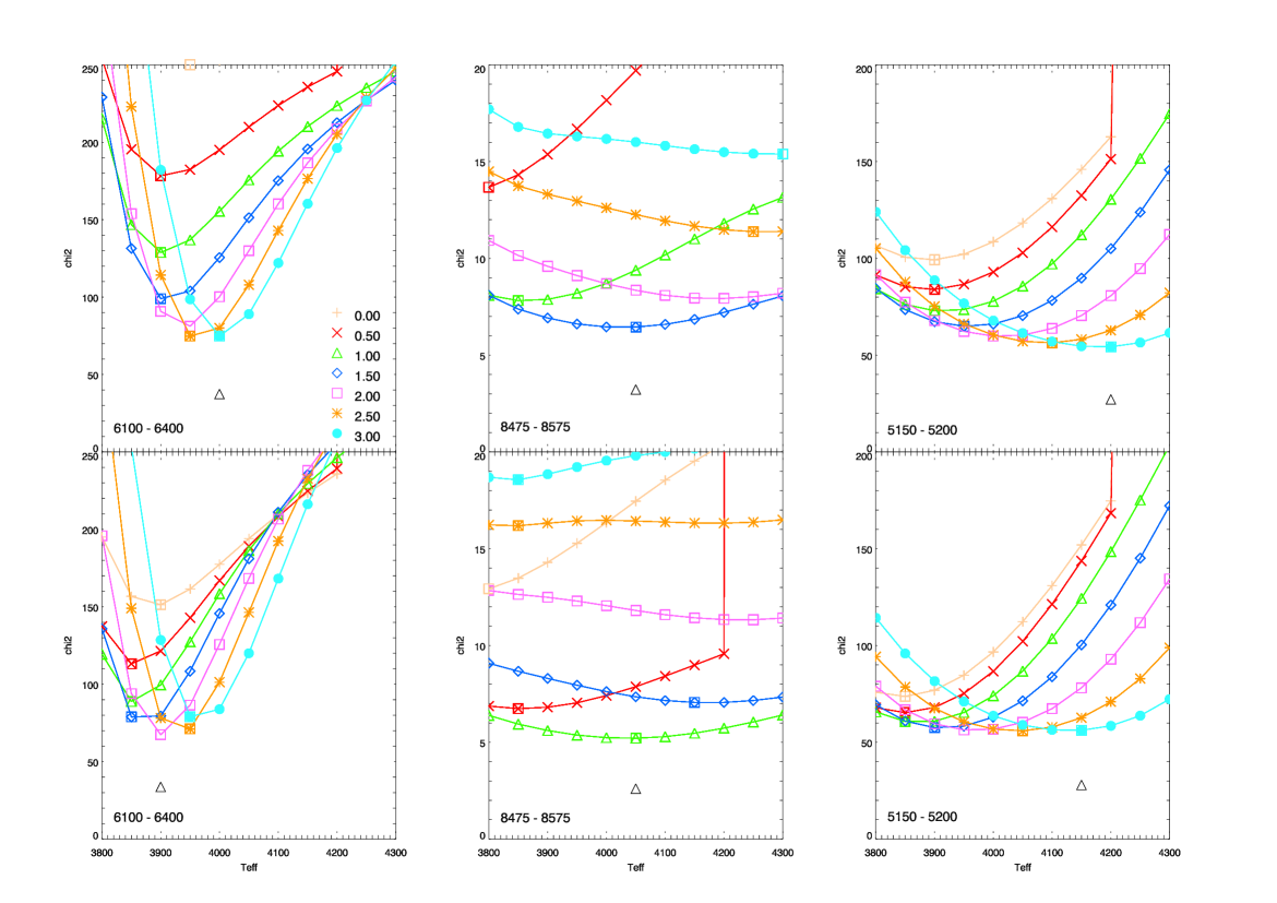
Figure 2: M4 analysis of Star 1: $\chi^{2}$ values as a function of $T_{\rm eff}$ for different $\log g$ values (see legend) and for three different wavelength regions (left, middle, right). Top row: solar abundances, bottom row: [Fe/H]= $-$0.25.

8400–8900 Å:

In this wavelength region, very interesting from a Gaia point of view, we find the Ca II infrared triplet, which is strong in cool giant stars. The $\chi^{2}$ plots for the 8475–8575 Å wavelength interval for solar abundances and for [Fe/H]= $-$0.25 can be found in Fig. 2 (top and bottom center, respectively). The best fit for solar abundances is shown in Fig. 3. This region is not very sensitive to the effective temperature, and quite sensitive to the surface gravity. Using a lower metal abundance resulted in a lower surface gravity.

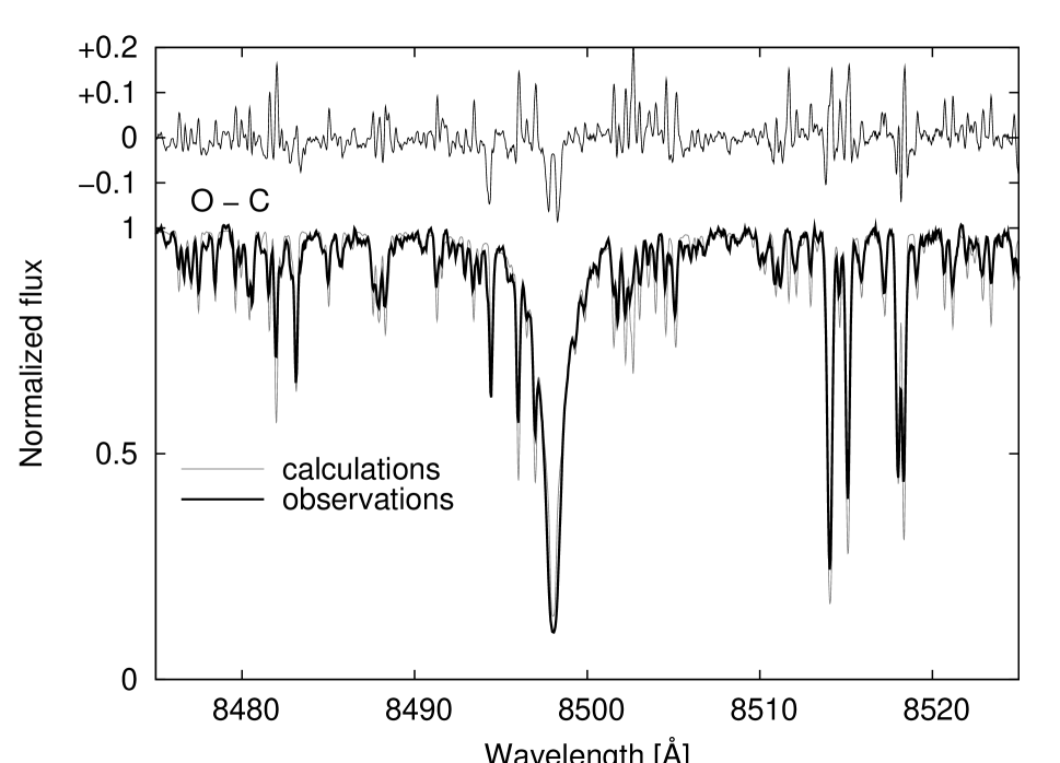
Figure 3: M4 analysis of Star 1: The best fit for the 8475–8575 Å region, showing a Ca II IR triplet line, for solar abundances ($T_{\rm eff}$=4050 K, $\log g$=1.5). Bottom: Scaled flux, observed and calculated; top: observed minus calculated flux.

4900–5400 Å:

This wavelength region has a much weaker temperature- and gravity sensitivity, as can be seen in Fig. 2 (right) for the interval 5150–5200 Å containing the Mg Ib triplet lines. The “best” fit for the [Fe/H]= $-$0.25 models is shown in Fig. 4.

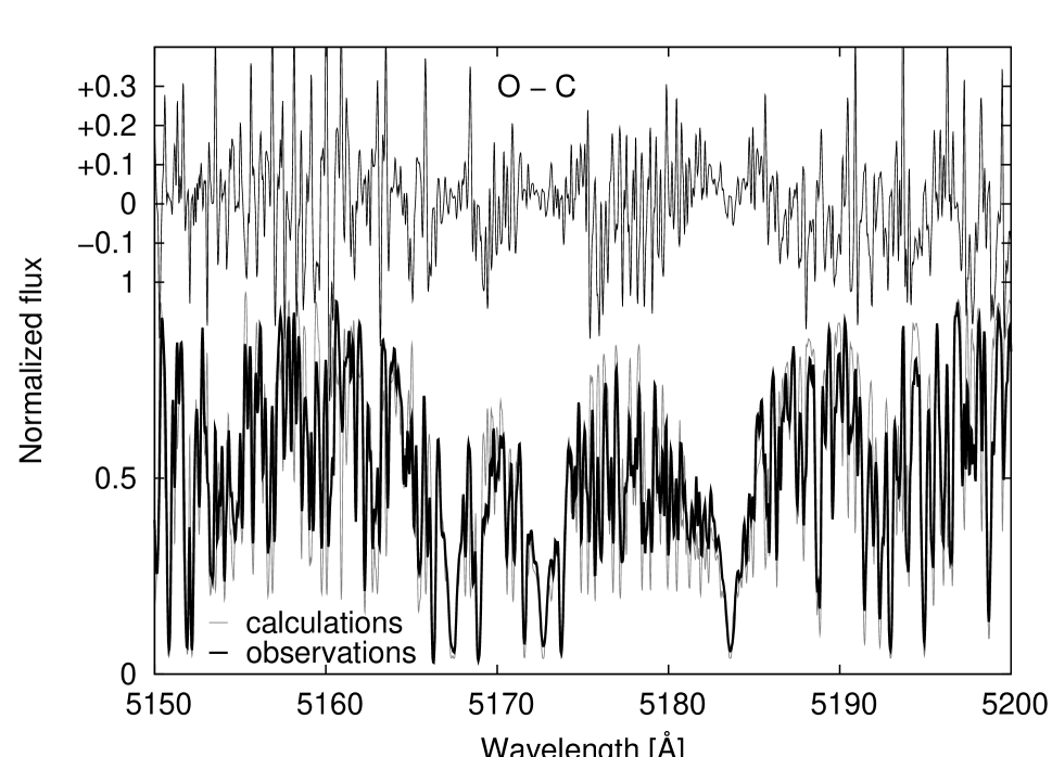
Figure 4: M4 analysis of Star 1: The best fit for the 5150–5200 Å region, showing the Mg Ib triplet lines, for sub-solar abundances ([Fe/H]= $-$0.25; $T_{\rm eff}$=4150 K, $\log g$=3.0). Bottom: Scaled flux, observed and calculated; top: observed minus calculated flux.

In conclusion, within the M4 analysis, the 6100–6400 Å region, with its temperature-sensitive TiO bands, was best suited for estimating the effective temperature for Star 1. The 8500 Å region was best suited for estimating the surface gravity. The solutions for the two adopted metallicity values are given in Table 12. It should be noted that the M4 analysis did not result in a unique set of best-fit parameters: the temperature-sensitive region gave a higher $\log g$ than the gravity-sensitive region, and vice versa. The blue-green region (5150–5200 Å) gave both a higher $T_{\rm eff}$ and a higher $\log g$ than the other two regions. Most of the other tested wavelength intervals behaved similarly to the blue-green region, i.e. showing very broad minima at rather high $T_{\rm eff}$ and $\log g$ in the $\chi^{2}$ plots. These were four 50–100 Å wide intervals between 4900 and 5400 Å, and a similar number of intervals in the region 8400–8900 Å, which did not contain any of the Ca II triplet lines.

An analysis of individual (e.g. Fe I) lines to derive an estimate of [Fe/H] was not attempted. Neither was a $\chi^{2}$ analysis in the metallicity dimension (although one can note that these values are on average somewhat smaller for the $-$0.25 models in Fig. 2). A further conclusion is that this procedure is to some degree dependent on the scale factors, i.e. it is important to have a good fit to the stellar continuum (which is hard to do, due to the effect of molecular bands).

3.1.5 M5

This part of the experiment was led by C. Abia. The M5 analysis focused on the coolest stars of the experiment, Star 3 and Star 4, because the M5 team members are more familiar with the spectral region to be analyzed in these stars (the $H$-band) where, furthermore, telluric lines are absent.

The original atomic line list was taken from the VALD database (version 2009). For the molecules, C₂ lines are from Wahlin & Plez (2005), CO lines come from Goorvitch (1994), an the CN and CH lines were assembled from the best available data as described in Hill et al. (2002) and Cayrel et al. (2004). The molecular lists also include lines of OH, TiO, CaH, SiH, FeH and H₂O taken from the HITRAN database (Rothman et al. 2005). First, the atomic and molecular lines were calibrated by obtaining astrophysical $gf$ values using the high resolution Solar (Livingston & Wallace 1991) and Arcturus (Hinkle et al. 1995) spectra in the 1.5$\mu$m region. In both analyses MARCS atmosphere models (Gustafsson et al. 2008) were used, with parameters $T_{\rm eff}$/$\log g$/[Fe/H]=5777/4.4/0.0 and 4300/1.5/$-$0.5 for the Sun and Arcturus, respectively. The reference abundances were those by Asplund et al. (2009) for the Sun, and those derived by Peterson et al. (1993) for Arcturus. The 1.5$\mu$m region is dominated by CO, OH, CN and C₂ absorptions (in order of decreasing importance). The main features were calibrated on the Arcturus spectrum. Synthetic spectra in LTE were computed using the TURBOSPECTRUM V9.02 code described in Alvarez & Plez (1998). The theoretical spectrum was convolved with a Gaussian function with a FWHM of $\sim$300 mÅ. The stellar parameters were estimated from the available photometry using the recent photometric calibrations by Worthey & Lee (2011) (see Tables 14 and 15).

Star 3:

A spherical (1 M_⊙) model atmosphere with parameters determined from the photometric colours was taken from the grid of Gustafsson et al. (2008). The fit (by eye) with this set of parameters to the observed spectrum was quite good in the full spectral range. The simultaneous fit to some OH, CO and CN lines allowed an estimate of the CNO abundances, namely C/N/O$=8.37/7.90/8.70$, i.e. C/O$=0.46$. A rough estimate of the metallicity from fits to some metallic lines in the region was compatible with [Fe/H] $\approx 0.0\pm 0.2$. Finally, according to the line list used, some CO lines are sensitive to variations in the ¹²C/¹³C ratio. Several fits unambiguously resulted in a carbon isotopic ratio lower than the solar value (89). However, due to the weakness of the ¹³CO lines only a lower limit was derived, ¹²C/¹³C$>25$.

Star 4:

With a model atmosphere with parameters determined from the photometric colours it was impossible to fit the observed spectrum. In particular, the predicted intensity of the CO lines was lower than observed. In this case, the stellar parameters were estimated through a $\chi^{2}$ test comparing observed and theoretical spectra computed for several choices of $T_{\rm eff}$/$\log g$/[Fe/H] ($\chi^{2}(i)\equiv\frac{(c(i)-o(i))^{2}}{c(i)+o(i)}$, where $c$ is the computed spectrum, and $o$ is the observed spectrum).

The best fit was obtained with a spherical 2 M_⊙ MARCS model (K. Eriksson, private communication) of parameters $T_{\rm eff}$/$\log g$/[Fe/H]= 3500/0.0/0.0 ($\chi^{2}<1.5$ over 20–30 Å regions). With these stellar parameters the corresponding photometric colours according to Worthey & Lee (2011) are instead $(V-I)$ = 2.49, $(J-K)$ = 1.18, and $(V-K)$ = 5.15. In the next step, the CNO abundances were estimated in a similar way to Star 3, resulting in C/N/O = $8.52/7.88/8.68$, i.e. C/O$=0.69$, and a lower limit of 35 for the ¹²C/¹³C. The estimated metallicity was also compatible with [Fe/H]$=0.0$. The microturbulence parameter was set to a fixed value (see Table 15). Note that the C/O ratio in the model atmosphere used (close to 1) was not consistent with the C/O ratio derived. The fact that this M-type star has some carbon enrichment may explain why a theoretical spectrum computed with the stellar parameters giving the best fit to the photometric colours does not fit the observed spectrum. In cool carbon enhanced stars, the actual C/O ratio is a critical parameter which determines the structure of the atmosphere affecting also the photometric colours. The results of the M5 analysis for both stars are summarized in Table 15.

3.1.6 M6

The M6 team, consisting of T. Merle and F. Thévenin, did not try to reproduce molecular lines and chosen to work with only Star 1  which has less affected spectra. For the M6 analysis, the photometry information was used to get starting values for $T_{\rm eff}$, $\log g$, and [Fe/H]. With the proposed approximate colours and using the theoretical calibrations by Houdashelt et al. (2000), the $T_{\rm eff}$ and $\log g$ values given in Table 12 were obtained. For K giant stars, a good approximation is to take a mass of 1 M_⊙. The spectroscopic analysis started with the selection of Fe I and Fe II lines. Care was taken to remove strong lines, multiplets with no dominant log $gf$ ($>$ 10%) and polluted or unclear line shapes in the observed spectrum. 21 Fe I lines were chosen in the near-IR range. Unfortunately, all Fe II lines in the near-IR part were too weak to use for a fit. Then, six Fe II lines were selected in the $[6100-6800]$Å range. For each line, radiative damping was estimated using the Unsöld formula; hydrogen elastic collisional damping came from ABO theory (Anstee & O’Mara 1995; Barklem & O’Mara 1997; Barklem et al. 1998) when available (e.g. the six Fe II lines), otherwise, classical Unsöld theory was used with an enhancement factor of 1.5 (e.g. the 21 Fe I lines). The line list is given in Table 6.

Table 6: Iron line selection for the M6 stellar parameter determination (Sect. 3.1.6). For each line, the wavelength $\lambda$, the lower level excitation potential $E_{\rm low}$, the $gf$ value, and the source for the $gf$ value are given.

$\lambda$	$E_{\rm low}$	log($gf$)	Sourcea
(nm)	(eV)
Fe I
843.957	4.549	$-0.587$	K07
847.174	4.956	$-1.037$	K07
852.667	4.913	$-0.760$	BWL
852.785	5.020	$-1.625$	K07
857.180	5.010	$-1.414$	K07
859.295	4.956	$-1.066$	K07
859.883	4.386	$-1.089$	BWL
860.105	5.112	$-1.577$	K07
861.394	4.988	$-1.247$	K07
863.241	4.103	$-2.341$	K07
869.945	4.955	$-0.380$	BWL
872.914	3.415	$-2.871$	K07
874.743	3.018	$-3.176$	K07
879.052	4.988	$-0.586$	BWL
879.807	4.985	$-1.895$	K07
881.451	5.067	$-1.793$	K07
881.689	4.988	$-2.203$	K07
883.402	4.218	$-2.558$	K07
884.674	5.010	$-0.777$	K07
889.140	5.334	$-1.108$	K07
Fe II
611.332	3.221	$-4.230$	RU
614.774	3.889	$-2.827$	RU
641.692	3.892	$-2.877$	RU
643.268	10.930	$-1.236$	RU
645.638	3.903	$-2.185$	RU
651.608	2.891	$-3.432$	RU

The final values of the stellar parameters for the M6 analysis were constrained by the method of ionization equilibria between Fe I and Fe II and excitation equilibria for Fe I. For this analysis, the MOOG2009 code (Sneden 1973) with spherical MARCS model atmospheres (Gustafsson et al. 2008) and atomic line lists from VALD were used. The inconsistency between spherical atmosphere and plane parallel radiative transfer is negligible (Heiter & Eriksson 2006). The chemical composition was from Grevesse et al. (2007). For each model atmosphere the abundance was determined for each line by fitting the observed spectrum while varying the iron abundance in steps of 0.1 dex around the abundance value adopted for the model atmosphere. The continuum level was determined using a local scaling factor. Then, [Fe I/H] was plotted as a function of the lower level excitation potential $E_{i}$ of the lines, and using linear regression, the model with the smallest slope was selected. For the ionization equilibrium, the mean [Fe I/H] and [Fe II/H] was compared for each model, and the model with the smallest abundance difference was selected. The best model atmosphere had parameters as given in Table 12. The uncertainties come from the large steps in the stellar parameters (200 K for $T_{\rm eff}$ , 1 for $\log g$ , and 0.1 dex in metallicity) taken to perform the analysis. With these large steps, the same atmospheric parameters were obtained both from the slope of [Fe/H] vs $E_{i}$ and from the ionization equilibrium.

The radial velocity was determined using 21 weak and relatively unblended lines in the $[6100-6800]$ and $[8400-8900]$ Å domains. The lines were synthesized using the MOOG2009 LTE code and shifted in steps of 0.5 km s^-1 for all the lines selected.

3.2 ATLAS model atmospheres (A)

3.2.1 A1

This working group consisted of G. Wahlgren and R. Norris. Using synthetic photometric colours from Kučinskas et al. (2005), initial estimates of temperature, gravity, and metallicity were made. With a least sum squares approach, the colours of the provided stars were compared to the colours in Kučinskas’ table, and the parameters of the best matching synthetic colours were interpolated to the given stars (see Tables 12 to 15).

Using these estimates of stellar parameters, appropriate ATLAS9 model atmospheres were selected from the grid of Castelli & Kurucz (2003), and synthetic spectra were created with SYNTHE (Kurucz 1993b). ATLAS is an LTE, plane-parallel model atmosphere code. Molecules from the Kurucz suite of line lists (Kurucz & Bell 1995, hydrides, CN, CO, TiO, SiO, H₂O) as well as other molecules were included in the statistical equilibrium calculations. The use of the gravities and metallicities obtained from broadband colours produced synthetic spectra which did not match the workshop spectra (at lines known to be sensitive to gravity and metallicity). Therefore, specific spectral lines as indicators of gravity and metallicity were used. The A1 analysis was continued for the K-type stars Star 1 and Star 3, because the contributing authors were not convinced that they had sufficient molecular opacities for late M-type stars.

Atomic line data in this analysis come from Kurucz (approximately 2008). Tables 7 and 8 list the lines used in the abundance determination for Star 1 and Star 3, respectively. Lines from neutral species only were used.

Star 1:

Synthetic colours suggested a cool, metal deficient giant or supergiant. Comparison to UVES spectra showed close matches with both HR 7971 (K3 II/III) and HR 611, which has ben classified as M0.8 III from narrow-band TiO/CN photometry (Wing 1978). The infrared Ca ii triplet (8498, 8542, 8662 Å) and the Fe i calibration lines at 8327, 8468, 8514, and 8689 Å noted in Keenan & Hynek (1945) were used to determine $\log g$ of 1.5 in a temperature range of 3900 – 4000 K. Deficiencies in iron (see Table 12) and the $\alpha$ elements were of particular note ([Si/H]=$-0.45\pm 0.03$, [Ca/H]=$-0.90\pm 0.15$, [Ti/H]=$-0.38\pm 0.03$). The lines used in these measurements are listed in Table 7.

Table 7: Lines used in the A1 analysis to determine abundances for Star 1. For each line, the atomic number $Z$, the wavelength $\lambda$, the $gf$ value, the lower level excitation potential $E_{\rm low}$, and the line abundance are given.

$Z$	$\lambda$	log($gf$)	Source	$E_{\rm low}$	Abundance
	(nm)			[cm-1]	(log(NH)=12.00)
14	568.448	$-$1.650	GARZ	39955.053	6.95
14	569.043	$-$1.870	GARZ	39760.285	7.10
14	570.110	$-$2.050	GARZ	39760.285	7.08
14	577.215	$-$1.750	GARZ	40991.884	7.04
14	579.307	$-$2.060	GARZ	39760.285	7.15
20	558.875	$+$0.210	NBS	20371.000	4.83
20	559.011	$-$0.710	NBS	20335.360	5.23
20	559.446	$-$0.050	NBS	20349.260	4.81
20	560.128	$-$0.690	NBS	20371.000	5.13
20	615.602	$-$2.200	NBS	20335.360	5.88
20	645.560	$-$1.350	NBS	20349.260	5.48
20	817.329	$-$0.546	K88	39349.080	5.90
20	820.375	$-$0.848	K88	36575.119	5.90
20	829.218	$-$0.391	K88	39340.080	5.80
22	546.047	$-$2.880	SK	386.874	4.55
22	556.271	$-$2.870	MFW	7255.369	4.55
22	802.484	$-$1.140	MFW	15156.787	4.45
22	806.825	$-$1.280	MFW	15108.121	4.65
22	841.229	$-$1.483	MFW	18482.860	4.55
22	867.527	$-$1.669	MFW	8602.340	4.50
22	868.299	$-$1.941	MFW	8492.421	4.50
22	869.233	$-$2.295	MFW	8436.618	4.70
22	873.471	$-$2.384	MFW	8492.421	4.70
26	552.554	$-$1.330	FMW	34121.580	6.70
26	552.890	$-$2.020	FMW	36079.366	7.30
26	552.916	$-$2.730	FMW	29371.811	7.10
26	553.275	$-$2.150	FMW	28819.946	6.70
26	554.394	$-$1.140	FMW	34017.098	6.70
26	555.798	$-$1.280	FMW	36079.366	6.65
26	556.021	$-$1.190	FMW	35767.561	6.75
26	829.351	$-$2.126	K88	38678.032	6.90
26	832.705	$-$1.525	FMW	17726.981	6.70

Of the $\alpha$ elements, the abundance of calcium resulting from the A1 analysis is particularly low. For the six lines below 8000 Å, which have a lower excitation energy close to 20 000 cm^-1, weaker $gf$-values correlated to higher abundances. For example, the 5589 Å and 5601 Å lines have the same lower excitation energy but have different $gf$-values. Of these, 5601 Å with a log($gf$)=$-$0.690 dex suggests an abundance of 5.13 whereas 5589 Åwith log($gf$)=0.210 dex suggests an abundance of 4.83. This trend does not exist for the three calcium lines above 8000 Å which were included in the abundance determination. Although each of these lines has a more energetic lower excitation energy, each suggests a higher abundance than the shorter wavelength lines with similar $gf$-values. These three lines use Kurucz (1988) calculated $gf$-values as opposed to the NBS (Wiese et al. 1969) values used for the shorter wavelength lines. The Kurucz (2007) calculated values for the four lines below 6000 Å have larger $gf$-values than NBS reports. Presuming that this correlation between calculated and experimental values would continue for longer wavelength lines, this indicates that for the three lines over 8000 Å, the reported $gf$-value is an upper bound. If the correlation between higher abundance and low $gf$-value in the shorter wavelength values is not entirely the result of poor atomic data; it is likely the result of non-LTE effects, to which calcium lines are particularly sensitive (for a non-LTE analysis of a different set of calcium lines see Section 5.3). The results of the A1 analysis for Star 1 are given in Table 12.

Star 3:

Synthetic colours suggested a metal deficient giant of effective temperature 4300–4400 K. Comparison of the workshop spectrum with synthetic spectra produced with parameters obtained from broadband colours showed that while the $\log g$ and temperature indicated by synthetic colours fit, the metallicity was closer to the solar value than the synthetic colours suggested. The A1 team determined abundances of carbon, nitrogen, and oxygen for Star 3 by fitting molecular lines. There are strong OH and CN lines present, as well as a CO bandhead, in the wavelength region of the experiment. Unblended OH lines were used as indicators of the oxygen abundance and CN and CO lines as indicators of carbon and nitrogen abundances. Several iron lines, listed in Table 8, served for the determination of the iron abundance. Despite hints from synthetic colours that the star was metal deficient, carbon, nitrogen, oxygen, and iron were all enhanced. Lines of some other elements, though not analyzed, suggested similarly enhanced abundances. The star was found to be oxygen rich. The results of the A1 analysis for Star 3 are summarized in Table 14.

Table 8: Fe I lines used in the A1 analysis to determine iron abundances for Star 3. For each line, the wavelength $\lambda$, the $gf$ value, the lower level excitation potential $E_{\rm low}$, and the line abundance are given.

$\lambda$	log($gf$)	Source	$E_{\rm low}$	Abundance
(nm)			[cm-1]	[log(NH)=12.00]
1549.034	$-$4.574	O	17726.987	7.85
1558.826	$+$0.323	K94	51359.489	7.70
1561.115	$-$3.822	K94	27523.001	7.65
1564.851	$-$0.714	K94	43763.977	7.90
1565.283	$-$0.476	K94	50377.905	7.80

3.2.2 A2

The A2 team (consisting of J. Maldonado, A. Mora, and B. Montesinos) decided to work only with the optical region of the spectrum, and therefore, only Star 1 and Star 2 were analyzed.

To determine the radial velocity, the spectra of the target stars were cross-correlated against spectra of several radial velocity standards (Maldonado et al. 2010). Cross-correlation was performed with the IRAF task fxcor. Spectral ranges with prominent telluric lines were excluded from the cross-correlation.

A grid of synthetic spectra was calculated for the parameter range given in Table 4. To compute the spectra, team A2 used ATLAS9 model atmospheres and the SYNTHE code (Kurucz 1993a, b), adapted to work under the Linux platform by Sbordone et al. (2004) and Sbordone (2005). Line data are from the Kurucz web site (2005 version). The following molecules are included: C₂, CH, CN, CO, H₂, MgH, NH, OH, SiH, SiO. Atomic line data are listed in Table $a$. The new opacitiy distribution functions from Castelli & Kurucz (2003) were used. A mixing length parameter of 1.25 was used. All spectra were computed with a resolution of 300 000,

To obtain the “best parameters” of the target stars, A2 compared the equivalent widths (EWs) of a sample of spectral lines measured in the target stars with the EWs of the same lines measured in each synthetic spectrum. To compile a list of “well behaved” lines, the A2 team calculated synthetic spectra for two stars with accurately known stellar parameters (namely, the Sun, G2V, and Procyon, F5IV) and compared them with high-resolution observed spectra. Relatively isolated lines, with a reasonable stretch of flat continuum around the limits, were selected to estimate the EWs with high accuracy. Since in all cases the synthetic lines fit the observed spectrum, it can be expected that the atomic parameters are fairly reliable. The list of lines used is given in Table $a$. The abundance ratios of the individual elements relative to each other were kept fixed to the solar ratios. Final parameters were obtained by using a reduced $\chi^{2}$ fitting method. Lines with large EWs ($>$100 mÅ) were not used. The results are listed in Tables 12 and 13.

The chosen method clearly can be further improved to obtain more accurate parameters. The first problem identified during the A2 analysis was the line selection. Although an attempt was made to compute a list of well behaved lines, it is clear that such a list depends on the spectral type of the target stars. The selection was started using as reference the Sun and Procyon, but some well behaved lines in the Sun were not well behaved in Procyon and vice versa. In addition, since the program stars of this experiment were cooler than the chosen reference stars, the selection had to be reviewed several times in order to avoid blended lines or lines not present in the program stars.

Table 9: Lines used by the A2 participants (Sect. 3.2.2). For each line, the species code, the wavelength $\lambda$ and the $gf$ value are given (taken from the line lists of Kurucz). Lines included in the final fit have been marked with the symbol ^⋆. The species code follows Kurucz’s notation, e.g. for iron lines (atomic number 26): 26.00 = Fe I, 26.01=Fe II, etc. References as listed in Kurucz & Bell (1995). Furthermore, the table gives the measured equivalent widths of the lines in the two benchmark stars.

Ion	$\lambda$	$\log$(gf)	Source	EW Star 1	EW star 2	Ion	$\lambda$	$\log$(gf)	Source	EW star 1	EW star 2
	(nm)			(mA)	(mA)		(nm)			(mA)	(mA)
26.00⋆	490.514	-2.050	FMW	73.63	30.33	26.00	536.162	-1.430	FMW	269.68	225.63
26.01	492.393	-1.320	FMW	–	–	26.00⋆	537.371	-0.860	FMW	82.82	97.37
26.00	492.477	-2.220	FMW	107.96	183.82	26.00	537.958	-1.480	FMW	102.03	113.47
24.00	493.634	-0.340	MFW	110.10	82.99	26.00	538.634	-1.770	FMW	–	–
26.00⋆	496.258	-1.290	FMW	52.201	–	26.00⋆	538.948	-0.410	FMW	20.50	85.97
28.00	501.094	-0.870	FMW	–	–	28.00	539.233	-1.320	FMW	–	4.94
26.00	504.422	-2.150	FMW	169.70	181.76	26.00	612.025	-5.950	FMW	112.24	113.17
26.00	504.982	-1.420	FMW	–	–	26.00⋆	615.938	-1.970	FMW	26.72	40.58
26.00⋆	505.465	-2.140	FMW	25.21	25.79	26.00	622.674	-2.220	FMW	23.82	6.31
22.00⋆	506.406	-0.270	MFW	2.45	2.50	26.01⋆	636.946	-4.253	K88	–	–
26.00⋆	508.334	-2.958	FMW	1.16	11.24	26.00⋆	639.254	-4.030	FMW	64.58	67.31
26.00	509.078	-0.400	FMW	–	4.39	21.01	660.460	-1.480	MFW	142.65	127.39
28.00⋆	509.441	-1.080	FMW	23.30	22.79	26.00⋆	672.536	-2.300	FMW	61.93	8.42
26.00⋆	512.735	-3.307	FMW	72.89	74.44	26.00⋆	848.198	-1.647	K94	39.32	30.20
26.00⋆	514.174	-2.150	FMW	73.17	91.99	14.00⋆	850.222	-1.260	KP	14.75	1.58
26.00⋆	514.373	-3.790	FMW	27.32	28.61	26.00	851.510	-2.073	O	152.76	132.81
22.00⋆	514.547	-0.574	MFW	–	–	26.00	858.225	-2.133	O	146.53	141.05
26.00⋆	515.191	-3.322	FMW	83.65	104.74	26.00⋆	859.295	-1.083	K94	83.14	81.46
26.00⋆	515.906	-0.820	FMW	74.80	80.40	14.00⋆	859.596	-1.040	KP	42.03	38.56
26.00	518.006	-1.260	FMW	–	–	14.00⋆	859.706	-1.370	KP	60.52	47.79
26.00⋆	518.791	-1.260	FMW	56.57	37.12	26.00⋆	859.882	-1.088	O	71.36	59.76
26.00	519.495	-2.090	FMW	73.31	113.68	26.00⋆	860.707	-1.463	K94	48.49	49.34
26.00⋆	519.547	0.018	K94	85.83	21.61	26.00	861.180	-1.900	FMW	217.20	226.04
22.01	521.154	-1.356	K88	–	–	26.00	862.160	-2.321	O	128.62	135.64
22.00⋆	521.970	-2.292	MFW	174.09	173.95	26.00⋆	867.474	-1.850	FMW	46.99	25.25
26.00	522.985	-0.241	K94	–	26.94	14.00	868.635	-1.200	KP	–	4.67
26.01	523.463	-2.050	FMW	–	–	26.00	868.862	-1.212	FMW	351.04	340.18
26.00	524.250	-0.840	FMW	114.71	172.90	26.00⋆	869.870	-3.433	K94	86.81	87.78
26.01⋆	525.693	-4.250	K88	57.75	–	26.00⋆	869.945	-0.380	O	77.67	69.31
26.00	526.331	-0.970	FMW	129.66	135.07	26.00⋆	871.039	-0.555	K94	87.34	86.76
24.00⋆	528.718	-0.907	MFW	61.55	19.62	14.00⋆	872.801	-0.610	KP	24.91	22.03
24.00	529.670	-1.400	MFW	214.13	203.87	26.00⋆	872.914	-2.951	K94	91.38	96.13
27.00⋆	535.205	0.060	FMW	62.30	50.28

This is related to the second problem, namely how to measure EWs. Although EWs can be measured “by hand” (for example using the IRAF task splot), this is not feasible even for this experiment with only two target stars, since more than six hundred synthetic spectra need to be analyzed. The A2 team developed a code which performs an integration around the center of each line using a fixed width. This could definitely be improved. Ideally, the code should be “intelligent enough” to decide on the width of the integration band according to the line profile. An alternative option, on which the A2 team is still working, is to compute EWs using model atmospheres and an abundance computation program such as WIDTH9 (Castelli 2005).

3.2.3 A3

For A3, H. Neilson attempted to determine the effective temperature, gravity, iron abundance, and carbon-to-oxygen ratio for Star 3 and Star 4 based on the broad-band colours and spectra provided. Model stellar atmospheres and synthetic spectra were computed using Fortran 90/95 versions of the ATLAS code (Lester & Neilson 2008). The new versions of the code can compute model stellar atmospheres assuming either plane-parallel or spherically symmetric geometry and either opacity distribution functions or opacity sampling. Lester & Neilson (2008) demonstrated that model stellar atmospheres computed with this code predict temperature structures consistent with plane-parallel ATLAS9 and ATLAS12 models as well as spherically symmetric PHOENIX (Hauschildt et al. 1999) and MARCS (Gustafsson et al. 2008) models. Furthermore, Neilson & Lester (2008) showed that spherical model atmospheres predict intensity distributions that fit interferometric observations of red giant stars (Wittkowski et al. 2004, 2006a, 2006b) with center-to-limb intensity profiles from model atmospheres, and they determined stellar parameters consistent with results using ATLAS9 and PHOENIX models.

For the A3 analysis, models were computed assuming plane-parallel geometry and using the opacity distribution functions to minimize computing time. Derivation of stellar parameters for the two stars was done in the following manner. First, synthetic colours were computed from a grid of model atmospheres spanning a range in $T_{\rm eff}$ of 3000 to 8000 K, and in $\log g$ of 0 to 3 with solar metallicity. Comparing the synthetic colours to the given colours, values for $T_{\rm eff}$ and $\log g$ were estimated. Next, a new grid of stellar model atmospheres and synthetic spectra for a range of $T_{\rm eff}$ and $\log g$ about the preliminary estimates was computed such that $\Delta$$T_{\rm eff}$ = $\pm 400$ K and $\Delta\log g=\pm 1$, while also varying the iron abundance. Line data were taken from Kurucz database. For each synthetic spectrum, a $\chi^{2}$-fit was computed and a new best-fit $T_{\rm eff}$, $\log g$, and [Fe/H] was determined. Using these values, a new grid was computed, varying $T_{\rm eff}$, $\log g$, and the silicon abundance. A new value for $T_{\rm eff}$  $\log g$, and the silicon abundance was found and the process was repeated for oxygen, carbon and calcium.

The best-fit stellar parameters for Star 3 and Star 4 resulting from the A3 analysis can be found in Tables 14 and 15. The results for Star 4 are consistent with the parameters given in Table 2. However, the results for Star 3 do not agree. This disagreement is due to the method which was employed. This method did not use any specific absorption lines to constrain the gravity or abundance. Instead, the parameters were determined using a blind $\chi^{2}$-fit. Furthermore, possible degeneracies between $\log g$ and various abundances were ignored. For instance, a synthetic spectrum for a model with $T_{\rm eff}$ = 4200 K, $\log g=2.25$, [Fe/H]$=0.6$ and C/O$=0.15$ had a fit to the Star 3 spectrum with a $\chi^{2}$ value that was $\lesssim 10\%$ different than the $\chi^{2}$ value for the best-fit model.

3.2.4 A4

A4 (R. Peterson) analyzed the optical spectrum of Star 1, as part of an ongoing analysis of standard stars spanning a wide range of temperature, gravity, and metallicity. For these analyses, stellar parameters and abundances were derived by matching each stellar spectral observation to theoretical spectra calculated with an updated version of the Kurucz (1993b) SYNTHE program and the static, one-dimensional stellar atmosphere models selected from the grid of Castelli & Kurucz (2003). A4 interpolated an appropriate model for each star, and used as input a list of molecular and atomic line transitions with species, wavelengths, energy levels, $gf$-values, and damping constants.

The Kurucz gfhy lists of atomic lines with known energy levels (“laboratory” lines) were modified by comparing calculations to echelle spectra of standard stars. Moving from weak-lined to stronger-lined stars, first each spectrum was calculated, then the $gf$- values were adjusted individually for atomic lines and as a function of band and energy for molecular lines, and, finally, a guess was made on the identifications of “missing” lines, those appearing in the spectra but not in the laboratory line list. This process was iterated until a match was achieved in each case. Peterson (2008) shows an example of the fits achieved in the near-UV for turnoff stars, from solar to extremely low metallicities. Fig. 5 shows optical spectra for stronger-lined stars.

Wavelength [Å]

Figure 5: A4 analysis: The plot compares observed spectra (heavy lines) to calculated spectra (light lines) for Star 1 and three standard stars. The two panels display two separate wavelength regions, as indicated in Å at the bottom of each panel. The stars are displaced vertically for clarity. Each y-axis tick denotes 10% of the full height of the normalized spectrum. The star name appears in bold above the continuum of each plot, followed by the model stellar parameters adopted for the calculation: effective temperature $T_{\rm eff}$, surface gravity $\log g$, logarithmic iron-to-hydrogen ratio [Fe/H] with respect to that of the Sun, and microturbulence $v_{\rm mic}$. Above the upper boundary of each panel appear identifications of the strongest lines in the calculation for $\mu$ Leo: the three digits after the decimal point of the wavelength in Å of the line is followed by a colon for a “missing” line, and then the species identification.

Stellar parameters were derived from the spectra, and not from colours. The effective temperature $T_{\rm eff}$ was constrained by demanding that the same abundance emerge from low- and high-excitation lines of the same species (usually Fe I), and by fitting the Balmer line wings in stars of $T_{\rm eff}$ $\sim$ 5000 K or hotter. The gravity was inferred from the wings of other strong lines; comparing Fe I and Fe II abundances provided a check. Demanding no trend in abundance with line strength set $v_{{\rm mic}}$. The iron abundance and other elemental abundance ratios stemmed from matching relatively unblended weak lines. The resulting uncertainties are typically 0.1 – 0.2 dex in [X/Fe] for element X. Peterson et al. (2001) provide details.

A4 first compared Star 1 against the metal-poor K1.5 III giant Arcturus ($\alpha$ Boo, HR 5340, HD 124897) and the super-metal-rich K2,III giant $\mu$ Leo (HR 3905, HD 85503), two well-observed stars. This quickly established Star 1 to be cooler than any giant with solar metallicity higher than one-third solar that A4 has analyzed before. Moreover, throughout the red region the star exhibited a multitude of absorption lines not seen in either of the other two K giants. The majority proved to be TiO lines. Consequently, the TiO line list of Schwenke (1998), downloaded from the Kurucz website was added.

Several iterations were required to fit reasonably well the observed spectrum for Star 1. The first iterations refined $T_{\rm eff}$, and simultaneously [Fe/H], then $\log g$ and $v_{\rm mic}$. Ultimately the best fit was obtained for a model with the parameters given in Table 12. The fit does deteriorate below 6000Å, where “missing” lines remain significant.

With one exception, there was no need to alter the relative abundance of any element with respect to that of iron in Star 1 from the values adopted for the Sun. For nitrogen in Star 1, however, the abundance was lowered to [N/Fe] = $-$0.1 dex to match the multitude of CN lines in the red. That oxygen in Star 1 is solar, [O/Fe] = 0, was confirmed from three separate diagnostics: the [O I] lines at 6300.3 Å and 6363.8 Å, the high-excitation O I triplet at 7771.9 Å, 7774.2 Å, and 7775.4 Å, and a fit of the red TiO lines. For the Sun the older, higher oxygen abundance log(O/H) = $-$3.07 was adopted.

For Arcturus and $\mu$ Leo, relative nitrogen abundances were increased by 0.1 dex. Relative abundances were also changed for other elements, notably sodium and aluminum, the light elements Ca, Mg, Si, and Ti, and elements beyond the iron peak, whose proportions are all known to vary among old stars (Sneden et al. 2008).

The degree to which the A4 calculations match the observed spectra of Star 1 and other standards is illustrated in Fig. 5, which shows a comparison in two wavelength regions of the observed spectrum to the calculated spectrum for four stars: the Sun, Arcturus, Star 1, and $\mu$ Leo. Both wavelength regions are relatively free of TiO absorption in Star 1, but its inclusion is nonetheless important to better define the continuum. Both have many CN features, which must be closely approximated to define both continuum and blends.

Although the match is not perfect, it is largely satisfactory in all four stars. Whenever a line is observed to be significantly too strong in one star, it is usually also significantly too strong in the others – indicating either a missing or wrong identification, or an erroneous $gf$-value. The Ca II core mismatch is due to the chromospheric contribution to this line. The $\log g$ values are supported by the agreement between Ca I and Ca II lines and by Fe II lines. Temperatures are supported by the wide range of lower excitation potentials spanned by lines of Si I, Ti I, and Fe I.

3.2.5 A5

The A5 analysis was performed by A. Goswami. The stellar atmospheric parameters ($T_{\rm eff}$, $\log g$, and [Fe/H]), for Star 1 were determined by an LTE analysis of the equivalent widths of atomic lines using a recent version of MOOG (Sneden 1973). The 59 cleanest lines of Fe I and two lines of Fe II within the three wavelength ranges recommended for Experiment 1 were used in the analysis (see Tab. $a$). The Fe lines covered a range in excitation potential (1.0 – 5.0 eV) and equivalent widths (10 – 165 mÅ). The excitation potentials and oscillator strengths of the lines were from various sources listed in the atomic spectral line database from CD-ROM 23 of R. L. Kurucz. Model atmospheres were selected from the Kurucz grid of model atmospheres available at the Kurucz web site. Kurucz models both with and without convective overshooting (see § 5.6) were employed, the latter from those that are computed with better opacities and abundances and labelled with the suffix “odfnew”. It was found that the derived temperatures from both the options agree well within the error limits.

Table 10: Lines analysed by A5 (Sect. 3.2.5). For each line, the wavelength, the $gf$ value, the lower level excitation potential $E_{\rm low}$, the equivalent width (EW), and the source of the line data according to Kurucz & Bell (1995) are given.

$\lambda$	$E_{\rm low}$	log($gf$)	EW	Reference
(nm)	(eV)		(mA)
Fe i
491.0325	4.191	-0.459	143.3	K88
491.6662	3.929	-2.960	26.8	FMW
491.8020	4.231	-1.360	68.9	FMW
492.7417	3.573	-1.990	78.1	FMW
494.5636	4.209	-1.510	82.5	FMW
495.2639	4.209	-1.665	73.6	K88
501.0300	2.559	-4.577	11.0	K88
505.8496	3.641	-2.830	45.1	FMW
513.7395	4.177	-0.400	116.9	FMW
523.6205	4.186	-1.720	51.3	FMW
526.2608	4.320	-2.280	30.4	FMW
530.0412	4.593	-1.750	19.1	FMW
531.5065	4.371	-1.550	70.2	FMW
532.2041	2.279	-3.030	156.2	FMW
532.6799	4.415	-2.100	31.5	FMW
536.4858	4.445	+0.230	136.7	FMW
538.5579	3.694	-2.970	32.9	FMW
538.6959	3.642	-2.624	84.9	K88
615.1617	2.176	-3.299	152.8	FMW
616.5361	4.143	-1.55	82.5	FMW
621.3429	2.223	-2.66	160.5	FMW
625.3829	4.733	-1.660	54.6	FMW
627.1276	3.332	-2.950	65.7	FMW
630.1498	3.653	-0.745	143.1	K88
630.2494	3.687	-1.203	112.1	K88
630.7856	3.642	-3.535	33.6	K88
631.5809	4.076	-1.710	72.3	FMW
632.2690	2.588	-2.426	151.1	FMW
633.6823	3.687	-1.050	145.7	FMW
640.8016	3.687	-1.048	161.0	K88
641.1647	3.653	-0.820	148.9	FMW
648.1869	2.279	-2.984	151.1	FMW
651.8365	2.830	-2.750	131.2	FMW
660.9110	2.559	-2.692	158.4	FMW
660.9676	0.990	-4.936	153.7	K88
663.3746	4.559	-0.780	81.4	FMW
664.6932	2.609	-3.990	81.6	FMW
664.8079	1.011	-5.275	118.3	FMW
666.3437	2.424	-2.479	161.5	FMW
666.7417	2.453	-4.400	56.7	FMW
670.3568	2.759	-3.160	100.2	FMW
670.5101	4.607	-1.496	63.1	K88
671.0316	1.484	-4.880	125.8	FMW
672.5353	4.103	-2.30	30.8	FMW
673.3151	4.638	-1.580	57.4	FMW
673.9520	1.557	-4.950	97.0	FMW
843.9563	4.549	-0.698	132.7	K88
847.1739	4.956	-0.863	67.7	K88
848.1982	4.187	-1.631	60.1	K88
852.6667	4.913	-0.513	86.4	K88
858.2257	2.991	-1.993	156.3	K88
859.8825	4.387	-1.428	75.8	K88
863.2412	4.104	-1.958	47.1	K88
878.4434	4.955	-1.393	52.8	K88
879.3338	4.608	-0.219	127.6	K88
880.4623	2.279	-3.234	162.0	FMW
886.6920	4.549	-0.065	157.9	K88
887.8248	2.991	-3.600	82.1	K88
Fe ii
528.4109	2.891	-3.190	56.4	FMW
645.6383	3.903	-2.075	45.2	K88

The microturbulence $v_{\rm mic}$ was estimated at a given effective temperature by demanding that there should be no dependence of the derived Fe I abundance upon the equivalent widths of Fe I lines (see Tables 12 and 13). The effective temperature was obtained adopting the derived value of the microturbulence parameter by the method of excitation balance, forcing the slope of the abundances from the Fe I lines versus excitation potential to be near zero. Using the Fe I/Fe II ionisation equilibrium, the surface gravity of the star was obtained. The results are listed in Table 12.

3.3 Phoenix model atmospheres (P)

A model fit using Version 15 of PHOENIX (Hauschildt & Baron 1999) was provided by C.I. Short. A grid of spherical LTE atmospheric models was computed with a parameter range as given in Table 4. The formal numerical precision for the fitting in $T_{\rm eff}$ was about $\pm 30$ K. The mass was held fixed at 1 M_⊙ to determine radii for each value of $\log g$. Convection was treated in the mixing length approximation with a mixing length parameter, $l$, of 1.0 pressure scale height. Atomic line data were taken from the ATLAS9 list (Kurucz 1993a). Most molecular line data are from Rothman et al. (2005) and Kurucz (1993a) except for the line lists of CO (Goorvitch 1994) and TiO (Schwenke 1998).

For the purpose of Experiment 1 the approach of investigating the global fit to two wavelength regions (“visible” and “near-IR”, see Fig. 1) was adopted in the P analysis. The radial velocity correction was determined by fitting the Doppler shift, $\Delta\lambda$, to relatively unblended weak spectral lines at the blue and red ends of the observed spectra. Synthetic spectra were computed with a spectral resolution, $R$, of 300 000. Assuming that giants are slowly enough rotating that vsini would be minor compared to the effect of microturbulence, no rotational broadening was taken into account. An initial rectification was performed by dividing the synthetic spectra by unblanketed spectra for each model; the spectra were then re-rectified to the observed spectra piece-wise with a single-point calibration in each of the two fitting regions. The visible region is affected by significant telluric contamination. In principle, every feature in the entire spectrum contains information about the stellar parameters, provided they can be modelled correctly, and this experiment can be seen as a test of how well a model “blindly” fitted to the broad spectrum with equal weight on all spectral lines would recover the stellar parameters of a known star.

In the near-IR region the strongest diagnostics are the Ca II IR triplet lines. However, it was found that PHOENIX consistently produces profiles for these lines that are too bright throughout the damping wings for any realistic stellar parameters, even with line damping parameters tuned to match the solar line profiles. A comparison of unblanketed spectra among the workshop participants revealed that PHOENIX predicts a larger “background” continuum flux throughout the near-IR band than the other codes, and a possibility to be investigated that is consistent with both of these results is that PHOENIX under-estimates the continuous opacity in this region.

Figure 6: P analysis: Relative flux difference, $(f_{\lambda,{\rm o}}-f_{\lambda,{\rm S}})/f_{\lambda,{\rm o}}$, smoothed to a resolution corresponding to $\Delta\lambda=50$ Å, for a subset of the grid with [M/H]=0.0 around the best-fit parameters for Star 1 are shown in gray-scale. The best-fit model (Teff/log g/[M/H] = 3940/2.0/0.0) is overplotted with a thicker line style.

Figure 6 shows the relative flux residuals, $(f_{\lambda},{\rm o}-f_{\lambda},{\rm s})/f_{\lambda},{\rm o}$, where $f_{\lambda},{\rm o}$ and $f_{\lambda},{\rm s}$ are observed and synthetic flux, respectively, for Star 1 and models of [M/H]= 0.0. Figures 7 and 8 show the values of $\chi^{\rm 2}$ per interpolated $\lambda$ point for Star 1 and Star 2, respectively, and all models.

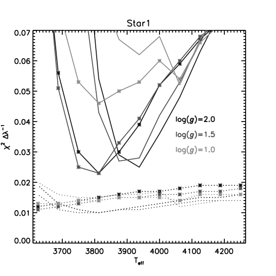
Figure 7: P analysis: Values of $\chi^{\rm 2}(\Delta\lambda)^{\rm-1}$ for Star 1. Solid lines: Fit to visible region; Dotted lines: Fit to near-IR region. No point symbol: [M/H]= 0.0; Asterisks: [M/H]= $-$0.5. Dark to light gray lines: $\log g$= 2.0 to 1.0.

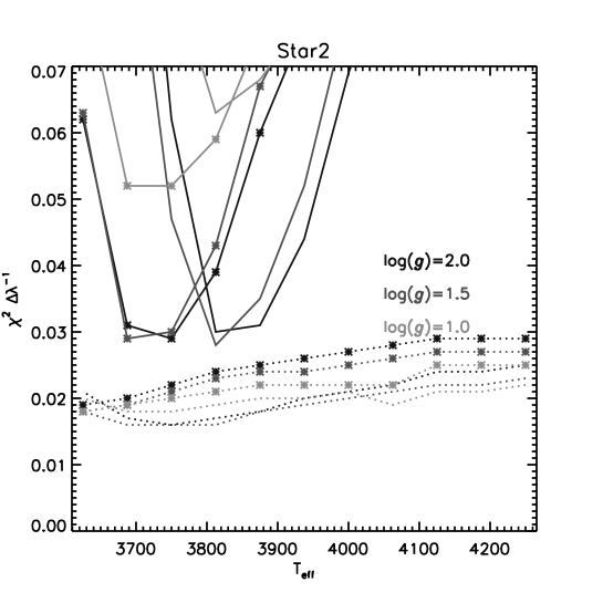
Figure 8: P analysis: Same as Fig. 7 except for Star 2.

Star 1

For the visible fitting region, the $\chi^{\rm 2}$ values showed distinct global minima as functions of $T_{\rm eff}$ (minimum $\chi^{\rm 2}(\Delta\lambda)^{\rm-1}\approx 0.025$), but picked out best-fit values of $\log g$ and [M/H] less clearly. Models of [M/H]=0.0 yielded best-fit $T_{\rm eff}$ values of 3940 and 3875 ($\pm 30$ K, formally) for $\log g$ values of 2.0 and 1.5, respectively. For [M/H]=$-$0.5 these $\log g$ values yielded best fit $T_{\rm eff}$ values of 3800 K. Models of $\log g$=1.0 provided a significantly worse fit. There was marginal evidence that models of [M/H]= $-$0.5 might provide a better fit than those of [M/H]= 0.0. For the near-IR region the $\chi^{\rm 2}$ values showed a much more shallow minimum around 3800 K (minimum $\chi^{\rm 2}(\Delta\lambda)^{\rm-1}\approx 0.01$) for [M/H]= 0.0 and $\log g$ values of 2.0 and 1.5, and did not show a minimum at all for [M/H]= $-$0.5.

Star 2

The fits yielded a similar result as that for Star 1, but with all the $\chi^{\rm 2}(\Delta\lambda)^{\rm-1}$ minima shifted downward in $T_{\rm eff}$ by about 100 K for the visible band, and 50 K for the near-IR band. For the visible band the best fit value for $\log g$ was either 1.5 or 2.0, and the best fit values for $T_{\rm eff}$ were 3800 K ([M/H]= 0.0) or 3700 to 3750 K ([M/H]= $-$0.5). Again, only models of [M/H]= 0.0 showed a minimum for the IR band, with a best fit $T_{\rm eff}$ value being indicated by a very shallow minimum of $\sim$3750 K. Models of [M/H] of 0.0 and $-$0.5 provided the same quality of fit, so the nominal best fit value was found to be $-0.25\pm 0.25$.

In conclusion, the near IR band needs attention in the P modelling to cultivate it as a more effective diagnostic of stellar parameters for M giants. The lack of distinct minima in the fitting statistic may be caused by the poor quality of the fit to the broad Ca II IR triplet lines, as discussed above. Therefore, the best-fit parameters for the P analysis given in Tables 12 and 13 are based entirely on the fit to the visible region.

3.4 CODEX model atmospheres (C)

The authors contributing the C analysis were M. Ireland and M. Scholz. The Cool Opacity-sampling Dynamic EXtended (CODEX) models as published in Ireland et al. (2008) are based on a combination of three separate codes – a grey dynamical atmosphere code, a temperature iteration code and a spectrum computation code. In addition, the equation of state is pre-tabulated based on the 1970s code from T. Tsuji, including updates from Sharp & Huebner (1990) and Jeong et al. (2003). The CODEX models are designed to predict the observables in the atmospheres of Mira variables, and the main algorithms involved are described in Schmid-Burgk (1975) and Schmid-Burgk & Scholz (1984). For the static models computed for this paper, the dynamical code was not used and the pressure stratification was iterated simultaneously with the temperature.

An important property of these models relevant to the test stars in this paper is that only atomic lines of neutral atoms were included, so that the code was not applicable and has not been used for effective temperatures above 4000 K. Furthermore, there were numerical instabilities that are not fully understood, which means that the spherical code could only be used in significantly extended configurations. In practice, this implied a restriction to $\log g$ values less than approximately $-$0.5 to 0. Within these constraints, the model structures produced by the CODEX models agree with MARCS structures within 50 K. The H2O lines come from Partridge & Schwenke (1997) and those of TiO from Schwenke (1998). Other diatomic molecular (CO, OH,CN, SiO, MgH) and neutral metal atomic lines come from the input to the ATLAS12 models (Kurucz 1994). VO was not taken into account here.

The full grid of models used to fit the stars in Experiment 1 had the parameters given in Table 4, and a fixed extension of 100 times solar. The atmospheric extension in this context was defined as $(T_{\rm eff}/5770)(R/{\rm R}_{\odot})(M/{\rm M}_{\odot})^{-1}$. A spectral fit was obtained at fixed gravity by minimising the mean square difference in between the model and the sample spectrum after interpolating bi-linearly in metallicity and effective temperature. Additional fit parameters were macroturbulence (or almost equivalently spectrograph resolution/stellar rotation velocity), radial velocity, continuum flux and continuum slope. A single continuous spectral window was used for the analysis of Star 2 (see Fig. 1).

The only stars for which reasonable spectral fits could be obtained were Star 2 and Star 4, as they were the only stars with parameters that were covered by the model grid. Uncertainties in the fitted parameters were not estimated in the C analysis, but fits were noticeably poorer by eye at parameters different by 0.2 dex in metallicity or 50 K in effective temperature, and so these can be taken as uncertainties. Gravity was not meaningfully constrained, but the $\log g$ value with the marginally better fit was chosen from the two available. The best-fit parameters are given in Tables 13 and 15. For Star 4, the broad band colours computed from the models are $V-I$=1.89, $J-K$=0.94 and $V-K$=3.71.

3.5 Tsuji08 model atmospheres (T)

The T analysis was provided by T. Tsuji. Modelling was restricted to Star 4, as the recent focus of the contributing author has been on the analysis of near infrared molecular lines (Tsuji 2008). With the given photometric data (see Table 2) it was not easy to infer fundamental parameters of this star. According to Perrin et al. (1998) $J-K=1.21$ corresponds to an M7 giant (see their Table 3), which would have a typical $T_{\rm eff}$ of 3087$\pm 94$ K (see their Table 5). $T_{\rm eff}$ = 3100 K was, thus, chosen for Star 4. In the absence of any information on mass, radius, etc. it was simply assumed that $M=2{\rm M}_{\odot}$ and $R=200{\rm R}_{\odot}$. These model parameters were adopted, together with a microturbulence $v_{\rm mic}$ = 3km s^-1, from a grid of model photospheres for red giant stars presented in Tsuji (2008). The abundance pattern used for the modelling is described in Table 4, case (b), in Tsuji (2008) for CNO and in Table 1 in Tsuji (2002) for other elements. Line data for CO 3–0 lines are listed in Table 11. Line positions and gf values are referenced in (Tsuji 2008). In particular, log $A_{\rm C}/A_{\rm H}$ = $-$3.92, log $A_{\rm N}/A_{\rm H}$ = $-$3.55, log $A_{\rm O}/A_{\rm H}$ = $-$3.31, and [Fe/H] = 0.0, were chosen.

For the abundance analysis, 14 CO lines relatively free from blending in the given spectrum of Star 4 were measured. The resulting equivalent width (EW) data are given in Table 11. A measurement of OH and CN lines was also attempted but it was difficult to find a sufficient number of lines free from disturbance. Line-by-line (LL) analysis as described in detail in Tsuji (1986, 2008) was applied to measure the selected CO lines. Results are shown in Fig. 9a, in which logarithmic abundance corrections to the assumed carbon abundance for different lines are given for $v_{\rm mic}$ = 3, 4, and 5 km s^-1. For the microturbulence value given in Table 15), the abundance corrections were found to be independent of EWs, and the mean logarithmic abundance correction was found to be $+0.36\pm 0.13$. This resulted in ${\rm log}A_{\rm C}/A_{\rm H}=-3.92+0.36=-3.56\pm 0.13$. Fig. 9b shows that the logarithmic abundance corrections are on average zero for these parameters.

Table 11: Measured CO 3–0 lines in Star 4 from the T analysis (Sect. 3.5). For each line, the wavelength $\lambda$ (air), the $gf$ value, the lower level excitation potential $E_{\rm low}$, the equivalent width over wavenumber log $W/\nu$, and the identification are given.

$\lambda$	log($gf$)	$E_{\rm low}$	log $W/\nu$	Identification
(nm)		[cm-1]
1560.082	$-$7.797	886.903	$-$4.696	12C16O 3–0 R 21
1560.447	$-$7.823	806.383	$-$4.632	12C16O 3–0 R 20
1560.839	$-$7.850	729.678	$-$4.691	12C16O 3–0 R 19
1561.257	$-$7.877	656.789	$-$4.679	12C16O 3–0 R 18
1561.533	$-$7.249	5055.604	$-$4.732	12C16O 3–0 R 51
1561.702	$-$7.907	587.721	$-$4.621	12C16O 3–0 R 17
1562.002	$-$7.234	5252.117	$-$4.784	12C16O 3–0 R 52
1562.499	$-$7.220	5452.275	$-$4.744	12C16O 3–0 R 53
1563.748	$-$8.038	349.698	$-$4.645	12C16O 3–0 R 13
1564.157	$-$7.179	6074.532	$-$4.791	12C16O 3–0 R 56
1564.326	$-$8.076	299.766	$-$4.695	12C16O 3–0 R 12
1564.930	$-$8.116	253.667	$-$4.707	12C16O 3–0 R 11
1565.561	$-$8.159	211.404	$-$4.729	12C16O 3–0 R 10
1566.763	$-$7.125	6954.739	$-$4.902	12C16O 3–0 R 60

Figure 9: T analysis: a) Line-by-line analysis of CO lines in Star 4, i.e. logarithmic abundance corrections to the assumed carbon abundance derived from the observed log $W/\nu$ values are plotted against the log $W/\nu$ values for $v_{\rm mic}$ = 3, 4, and 5 km s^-1. b) Confirmation of the null abundance corrections for ${\rm log}A_{\rm C}/A_{\rm H}=-3.56$ and $v_{\rm mic}=3.93$ km s^-1.

For the resulting microturbulence and carbon abundance, a synthetic spectrum for the region of the CO 3–0 band was computed, and the result is compared with the observed one in Fig. 10a. The CO lines used in the LL analysis are indicated by the rotational identifications for the CO 3–0 lines. Only these CO lines should be considered for estimating the quality of the fit, but fits are not so good even for these lines. To improve the fits in Fig. 10b, some additional broadening may be required, and several values of macroturbulent velocities were tried. It was found that the fits are somewhat improved for the selected CO lines with an assumed macroturbulent velocity of 3.0 km s${-1}$ (which could have been determined empirically if a sufficient number of weak lines could be measured, as in Fig. 3 in Tsuji (1986)).

Figure 10: T analysis: a) Observed spectrum (dots, relative flux vs. wave number) and model spectrum (solid line) with a macroturbulence of zero, for the CO lines between 1.5601 and 1.5625 $\mu$m of Star 4. b) The same as a) but with a macroturbulence of 3.0 km s^-1.

Because the stellar parameters ($T_{\rm eff},M,R$ etc.) cannot be pre-defined well and because the number of lines is too small for the LL analysis, only the basic procedure to analyze the stellar spectrum has been shown and a final converged solution was not pursued. However, we may conclude that the abundance determination is possible even for very cool stars in this way, if dozens of weak lines could be measured.

For the T analysis, the classical theory of line formation assuming the presence of microturbulence was applied. However, the applicability of the classical model of line formation may be limited to relatively weak lines with log $W/\nu<-4.75$ (Tsuji 2008). Although the sample of CO lines of Star 4 analyzed here includes some lines slightly stronger than this limit, the modelling was quite successful because most of the lines used are weak and below or near the limit mentioned (Tsuji 1991, cf. a similar previous study of the CO second overtone lines). The strongest lines with log $W/\nu>-4.5$ clearly deserve an extra contributions from outside the photosphere (Tsuji 1988). Thus, if a large number of the intermediate strength lines with $-4.75<{\rm log}\,W/\nu<-4.5$ are included as in a previous study of the CO first overtone lines (Tsuji 1986), the results cannot be correct as was recognized 20 years later (Tsuji 2008). Such a problem will appear not only in very cool stars but also in earlier type stars such as K giants (Tsuji 2009).

4 Results

As described above, two experiments were conducted. Experiment 1 had the aim to find the best fitting model to the four sample spectra provided, using the preferred method of each participating researcher or team. It was to be completed before the beginning of the workshop. A time limit of several weeks was set for the groups to deliver their results. This limit was introduced not only for practical reasons but also to simulate the typical amount of time used for parameter determination from a stellar spectrum in the current age of multi-object spectrographs and large surveys. Naturally, this time limit set some constraints on the level of elaboration of the resulting fits. Experiment 2 resulted from the discussions at the workshop and was aimed at a direct comparison of synthetic spectra from different model codes for a given set of stellar parameters.

4.1 Experiment 1 – stellar parameter determination

We start with an overview of the main aspects of the different modelling approaches (for details see Sections 3.1 to 3.5). About half of the groups (six of fourteen) based their analysis on MARCS atmospheric models calculated in spherically-symmetric geometry. Five groups used the plane-parallel ATLAS suite of codes (Kurucz 1993a, b; Lester & Neilson 2008). The three software packages PHOENIX (Hauschildt & Baron 1999), CODEX (Ireland et al. 2008) and Tsuji08 (Tsuji 2008) were employed by one group each (all of them spherical). The first character of the group identifier indicates this aspect. The stellar radius, a key parameter, is defined as the layer where the Rosseland optical depth is equal to one in the case of the MARCS models, the model of Tsuji, and the CODEX models. In the case of the PHOENIX models, it is assumed that the stellar mass $M$ is one solar mass, and the radius $R$ is computed accordingly from the specified surface gravity ($R=(GM/g)^{1/2}$). For the plane-parallel ATLAS models the radius is undefined.

To improve the fit of the line widths and to take into account various additional line broadening mechanisms like stellar rotation a macroturbulence has been added by most of the groups, i.e. the synthetic spectra have been convoled with a Gaussian profile.

The set-up did not require all participants to complete the experiment for all four spectra. Indeed, due to methodological constraints, some participants restricted their attempts to either the visual (M2, M3, M4, M6, A2, A4, A5, P) or the near infrared spectra (M5, A3, T). Naturally, the team that prepared the artificial observations for Star 3 and Star 4 (M1) did not participate in the fitting of these spectra. Two groups analysed both wavelength domains – A1 (Star 1 and Star 3) and C (Star 2 and Star 4). In summary, Star 1 was analysed by eleven groups, of which five also analysed Star 2. Star 3 and/or Star 4 were analysed by five groups.

Figure 11: Results of the various model fits in three different two-parameter planes for Star 1 ($\alpha$ Tau). The red star marks the values of the direct parameters given in Table 1.

4.2 $\alpha$ Tau (Star 1) and $\alpha$ Cet (Star 2)

The best fits to these two spectra as provided by the participating teams are summarized in Tables 12 and 13. For $\alpha$ Tau we have the more extensive set of model fits. The results are presented in Fig. 11 for the three possible combinations of the three main parameters derived: $T_{\rm eff}$, $\log g$, and [Fe/H]. The (unweighted) mean values of all results are: $T_{\rm eff}$ = 3980$\pm$250 K, $\log g$ = 1.3$\pm$0.3, and [Fe/H] = $-$0.2$\pm$0.2 dex, close to the literature values discussed in Section 2.2 and Table 1. No systematic differences between the model families (MARCS, ATLAS, and others) are apparent. Within the error bars given by the different groups, the derived $T_{\rm eff}$ values of almost all groups agree with each other. The only exception is the A2 analysis, which deviates by 800 K from the mean value. Discarding the A2 value, the mean $T_{\rm eff}$ of $\alpha$ Tau as a result of this experiment becomes 3910$\pm$80 K. Note that in the case of our experiment, contrary to a series of repeated measurements, the mean value does not necessarily result in a more precise value than the individual determinations.

We have no obvious explanation for the deviating result of A2, but the analysis approach differs in various aspects from the bulk of the other analyses. First, A2 uses a large model atmosphere grid including $T_{\rm eff}$ values up to 6000 K, which makes it possible to probe higher temperatures than other analyses. However, the same can be said for the M3a and M3b analyses, which do not find a high-$T_{\rm eff}$ solution using a grid up to 8000 K. Second, A2 did not include molecular lines in the analysis, but the same is true for M6, A1, and A5. A final aspect is that A2 did an equivalent width analysis, and not a synthetic spectrum fit, which seems problematic when dealing with crowded spectra. The A5 analysis also used equivalent widths, and obtained a $T_{\rm eff}$ close to the mean value. However, there are important differences between the two analyses, which might explain the different results. A2 measured equivalent widths for selected lines of several different species from the observed and computed spectra, while A5 computed equivalent widths line-by-line, adjusting the abundances for lines of Fe I and Fe II only. Also, A2 derived all parameters simultaneously from a fit to all lines, while A5 used the classical approach of excitation and ionization equilibrium for Fe lines. Note that there are only three lines in common in the line lists of A2 and A5.

Concerning gravity, the results for $\alpha$ Tau group around two values, slightly lower (M1, M3b, M6, A4, A5) and slightly higher (M2, M3a, A1, A2, P) than the published values given in Table 1, with the two M4 results falling in both groups. The majority of the modelers found $\alpha$ Tau to exhibit a lower metallicity than the Sun, the lowest values being suggested by A1. For the cases where [Ca/Fe] values were also determined, most groups find a mild underabundance of Ca.

Figure 12 shows the best-fit $T_{\rm eff}$ and $\log g$ for Star 1 ($\alpha$ Tau) from all participants except A2 converted to luminosity, using three different mass values, together with the direct $T_{\rm eff}$ and $\log g$ values from Table 1. We also show evolutionary tracks for metal-poor models by the Padova group for several different mass values. It is obvious that some of the derived pairs of parameters are inconsistent with the chosen stellar evolution models.

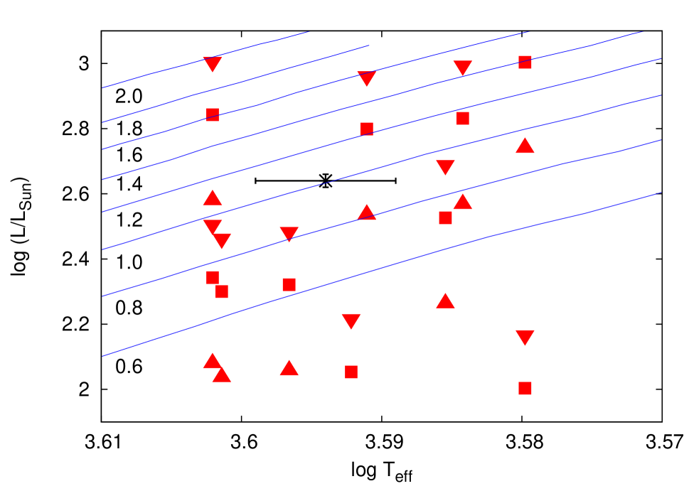
Figure 12: Best-fit $T_{\rm eff}$ and $\log g$ for Star 1 ($\alpha$ Tau) converted to luminosity, using three different mass values (triangles up – 0.6 $M_{\odot}$, squares – 1.1 $M_{\odot}$, triangles down – 1.6 $M_{\odot}$), and direct $T_{\rm eff}$ and $\log g$ values from Table 1 (black cross with error bars). Solid lines are evolutionary tracks for $Z$=0.008 and $Y$=0.26 by the Padova group (Bertelli et al. 2008, 2009), labelled to the left with mass in solar masses.

Fewer model fits are available for $\alpha$ Cet, and thus we have omitted a graphical presentation. The (unweighted) mean values and standard deviations of all results are: $T_{\rm eff}$ = 3830$\pm$220 K, $\log g$ = 1.0$\pm$0.8, and [Fe/H] = $-$0.2$\pm$0.2 dex, which is close to the published values discussed in Section 2.3. As for $\alpha$ Tau we find rather good agreement in the derived temperature, with the exception of A2 (deviating by 500 K). Discarding the A2 value, the mean $T_{\rm eff}$ of $\alpha$ Cet as a result of this experiment becomes 3760$\pm$70 K. Concerning the surface gravity, the scatter is somewhat larger than for $\alpha$ Tau, and the majority of the values are larger than the published value. For [Fe/H] the model fits to the spectrum of $\alpha$ Cet suggest metallicities from solar to subsolar. In general, one would expect a correlation between $T_{\rm eff}$ and [Fe/H] for the differing results, since line strength increases towards lower temperatures and higher [Fe/H]. This can be seen to some extent in Fig. 11, and the $\alpha$ Cet results show a similar trend. On the other hand, there is no obvious correlation between $\log g$ and $T_{\rm eff}$, or $\log g$ and [Fe/H].

Table 12: Experiment 1: parameters determined for $\alpha$ Tau (Star 1) from the best fits to the optical spectra by the various participating teams.

	starting parameters from photometry			best fit parameters from spectroscopy				additional quantities
Code	$T_{\rm eff}$	log $g$	[Fe/H]	$T_{\rm eff}$	log $g$	[Fe/H]	[Ca/Fe]	RV	$v_{{\rm mic}}$	$v_{{\rm mac}}$
	(K)	($g$ (cm s-2))		(K)	($g$ (cm s-2))			(km s-1)	(km s-1)	(km s-1)
M1			$-$0.3	3800$\pm$100	0.75$\pm$0.25	$-$0.3$\pm$0.25		54	2.5	3
M2	3850/4000			3850	1.25	0.0	0.0$\pm$0.1	54.5	1–2	4.5
M3a				3994$\pm$100	1.54$\pm$0.20	$-$0.15$\pm$0.10		53.9$\pm$0.9	2
M3b				3839$\pm$80	0.94$\pm$0.15	$-$0.35$\pm$0.10	$-$0.2$\pm$0.1	53.9$\pm$0.9	2
M4				4000	1.5	0.0		55	2	0
				3900	1.0	$-$0.25		55	2	0
M6	3750–4250	1.0–1.5		4000$\pm$200	1.0$\pm$1.0	0.0$\pm$0.5	$-$0.3$\pm$0.1	54.3$\pm$0.5	2
A1	3900	0.0	1.0	3950$\pm$100	1.5	$-$0.67$\pm$0.08	$-$0.23$\pm$0.17		2	–
A2				4788$\pm$92	1.5$\pm$0.1	$-$0.4$\pm$0.1		54.1$\pm$0.4	2
A4				3900	1.0	0.0		54.3	1.3	1.5
A5				4000$\pm$200	1.0$\pm$0.25	$-$0.29			1.6$\pm$0.5
P				3910$\pm$45	1.75$\pm$0.25	0.0		54.71	3	0
				3800$\pm$30	1.75$\pm$0.25	$-$0.5		54.71	3	0

Table 13: Experiment 1: parameters determined for $\alpha$ Cet from the best fits to the optical spectra by the various participating teams.

	starting parameters from photometry			best fit parameters from spectroscopy				additional quantities
Code	$T_{\rm eff}$	log $g$	[Fe/H]	$T_{\rm eff}$	log $g$	[Fe/H]	[Ca/Fe]	RV	$v_{{\rm mic}}$	$v_{{\rm mac}}$
	(K)	($g$ (cm s-2))		(K)	($g$ (cm s-2))			(km s-1)	(km s-1)	(km s-1)
M1			$-$0.5	3675$\pm$50	0.5$\pm$0.25	$-$0.5$\pm$0.2			2.5	3
M2	$\lesssim$3700			3700	1.0	0.0		$-$25.9	1–2	5.0
M3a				3867$\pm$100	1.15$\pm$0.20	$-$0.22$\pm$0.10		$-$27.6$\pm$1.3	2
M3b				3718$\pm$80	1.31$\pm$0.15	$-$0.02$\pm$0.10	$-$0.32$\pm$0.10	$-$27.6$\pm$1.3	2
A1	3500	1.0	$-$2.0
A2				4310$\pm$136	1.5$\pm$0.1	$-$0.6$\pm$0.1		$-$26.3$\pm$0.4	2
P				3750$\pm$30	1.75$\pm$0.25	$-$0.25$\pm$0.25		$-$26.22	3	0
C				3820$\pm$50	$-$0.5	0.0$\pm$0.2			2.8	2.3

4.3 Star 3 and Star 4

The fitting results for the two artificial stars are summarized in Tables 14 and 15. In this part of the experiment we asked the participants to derive also a C/O ratio.

The fitting of spectra in the optical range is still more widely used than the application of the same technique to spectra in the $H$ and $K$ band. This may be due to the longer and wider availability of optical high-resolution spectrographs and the better knowledge of the resident features. It is therefore not surprising that also the number of teams providing a fit to one of the near-infrared spectra is smaller than for the case of the optical ones. Furthermore, the lower temperature, especially of Star 4, requires an extensive inclusion of molecular line data, which is not needed for the usual work of some of our participating teams and, therefore, not included in their codes.

In comparing the fit results with each other we have to remember that the fitted star’ was a MARCS model. Therefore, one could expect that systematic differences between the underlying codes of the model fits should show up more clearly. For Star 3 the result is a bit surprising, because the best fits of all three groups gave a solar or supersolar metallicity, while the Star 3 model is clearly subsolar. Also, the derived C/O ratio differs significantly from the model input value. Temperature values, on the other hand, nicely agree with each other and are in reasonable agreement with the Star 3 value. For Star 4, all model fits are close to the real values or at least point into the correct direction (in particular to a higher C/O ratio).

A conclusion may be that the spectra of cool stars can be understood reasonably well if the attention is confined to relatively weak lines. However, we are still far from understanding complete spectra of cool stars including the intermediate strength lines and the strong lines, and the status of the modelling of these strong lines is still not at a satisfying stage. It appears to be no problem in analyzing the CO lines in Star 4, but this may be simply because the provided spectrum of Star 4 does not include strong lines, and we should not be fully satisfied with the present result.

Table 14: Experiment 1: parameters determined for the artificial spectrum of Star 3 from the best fits of the various participating teams.

	starting parameters from photometry			best fit parameters from spectroscopy
Code	$T_{\rm eff}$	log $g$	[Fe/H]	$T_{\rm eff}$	log $g$	[Fe/H]	C/O	$v_{{\rm mic}}$	$v_{{\rm mac}}$
	(K)	($g$ (cm s-2))		(K)	($g$ (cm s-2))			(km s-1)	(km s-1)
M2	4225
M5	4250	2.0	0.0	4250	2.0	0.0	0.46	1.7	4.5
A1	4300	2.0	$-$2.5	4350$\pm$100	2.0	0.32$\pm$0.04	0.63	2	–
A3	4200	3.0	0.0	4400	3.5	0.6	0.63	2.0

Table 15: Experiment 1: parameters determined for the artificial spectrum of Star 4 from the best fits of the various participating teams.

	starting parameters from photometry			best fit parameters from spectroscopy
Code	$T_{\rm eff}$	log $g$	[Fe/H]	$T_{\rm eff}$	log $g$	[Fe/H]	C/O	$v_{{\rm mic}}$	$v_{{\rm mac}}$
	(K)	($g$ (cm s-2))		(K)	($g$ (cm s-2))			(km s-1)	(km s-1)
M2	$\gtrsim$3300 K/3500 K
M5	3250	0.0	0.0	3500	0.0	0.0	0.69	3.0	5.0
A1	3800	1.0	$-$1.5
A3	3000	1.0	0.0	3200	0.25	0	0.79	2.0	0
C				3244$\pm$50	0.0	$-$0.1$\pm$0.2	0.48	2.8	1.2
T	3087$\pm$94			3100	0.14	0.0	0.56	3.9$\pm$0.4	3.0

4.4 Experiment 2 – synthetic spectra comparison

For Experiment 2 the participants were asked to calculate a synthetic spectrum using the stellar parameters listed in Sect. 2.4. Spectra should be provided for the wavelength ranges 4900–5400 Å, 6100–6800 Å, and 8400–8900 Å, respectively. Eight high-resolution spectra ($R$=300 000 to 500 000) were produced for the comparison, namely P, A1, A2, A3, M1, M2, M3, and M4. Note that M3 is at that stage (no parameter determination) very similar to M2 since the spectra are based on the same line-lists and model atmospheres but due to interpolation and the selected parameters the spectra are slightly different. A3 provided both a plane-parallel and a spherical solution, which are very similar. The plane-parallel version is used in the following as it had the higher spectral resolution. A1 and A2 both used ATLAS9+SYNTHE, but under two different operating systems. They differ only at very few wavelength points, so that we show only A1 in the figures below. An overview of the modelling details can be found in Table 16.

Table 16: Overview of model inputs used for Experiment 2. The listed codes were also used for Experiment 1.

Label	Codes	Spectral	Comments
		resolution
M1	MARCS + coma08	300000	spherical
M2	MARCS	500000	mass = 1 M⊙; spherical
	+ TURBOSPECTRUM
M3	MARCS	500000	mass = 1 M⊙, $\log g$=1.5, [Fe/H]=$-$0.25
	+ TURBOSPECTRUM		spherical
M4	MARCS + BSYN	300000 at 6000 Å	mass = 2 M⊙, $v_{{\rm mic}}$=2 km s-1; spherical
			spectrum convolved to a resolution of 80 000
A1	ATLAS9 + SYNTHE	500000	model atmospheres interpolated within Kurucz grid
A2	ATLAS9 + SYNTHE	300000	model atmospheres and spectra calculated
	Linux vers. (Sbordone)		for [Fe/H]=0 and $-$0.5, interpolated to [Fe/H]=$-$0.2
A3	ATLAS12	500000	plane-parallel
P	Phoenix V.15	300000

To compare these synthetic spectra we first made a linear interpolation of the normalized flux values to a common wavelength grid with a step size of 0.01 Å. Then, for each wavelength point the mean flux of all six spectra (P, A1, A3, M1, M2, M4) was calculated, and the root-mean-square (rms) difference of all normalized fluxes from the mean normalized flux was determined. Next, the rms differences were averaged over 2 Å-wide wavelength intervals. In addition, the difference of each individual normalized spectrum from the mean normalized flux was calculated.

Figure 13: Root-mean-square (rms) of the differences between the normalized flux of six model spectra (P, A1/A2, A3, M1, M2/M3, M4) and the mean of these six spectra, averaged over 2 Å-wide wavelength intervals. The different panels show four different wavelength regions, referred to in the text.

Figure 13 shows the rms flux differences. We note that a large rms value can be caused by one or more of the following: a large difference for an individual line, small differences for several lines, or a small continuum difference. To explore the features seen in Figure 13, we looked at the individual spectra in more detail. In Fig. 14 we show the differences of the six spectra from the mean, for selected 10 Å-wide wavelength intervals. Starting with Region 1 in Fig. 13, we found that MgH is the dominant molecular absorber in the region from 5000 to 5210 Å, where we see high rms differences. Comparison with a spectrum calculated with MgH lines only demonstrated that the differences in the spectra produced by different investigators are mainly due to differences in the MgH line data that they used. The broad rms peaks around 6220 Å in Region 2a and around 6740 Å in Region 2b coincide with regions where TiO absorption dominates, while the smaller peak around 6510 Å in Region 2b coincides with dominant CN absorption.

The three sharp peaks in Region 2a close to 6350 Å are due to three atomic lines. Two lines at 6343 and 6362 Å are present in four out of the six spectra, and are much broader in the A3 model than in the others. These lines are not present in the observed spectrum of $\alpha$ Tau. One line at 6354 Å is present in all models, but with varying line depths (0.3, 0.4, 0.6, 0.8, 0.9) – a comparison with the observed spectrum of $\alpha$ Tau points towards intermediate values. A careful check of the line lists revealed that these three lines can likely be associated with wrong data for some Ca i transitions. A3 included theoretical iron line lists from Kurucz, which are based on predicted energy levels. These lines appear to cause the strong and broad features seen in A3’s synthetic spectra at the mentioned wavelengths. A minor sharp peak can be seen in Region 2b close to the H$\alpha$ line, which was not included in the line list of the M2/M3 model (see Fig. 14b). We note that none of the models reproduce the H$\alpha$ line in the observed spectrum of $\alpha$ Tau. The observed line depth is more than twice as large as any of the calculated ones. In Region 3 in Fig. 13, the most obvious features are centered on the IR Ca II triplet lines and are due to different modelling of the broadening of these lines. A3 and M2/M3 show the broadest lines, A1/A2, M1, and M4 are narrower, and P is narrowest. An example is shown in Fig. 14c. Finally, the very sharp peak seen in Region 3 in Fig. 13 close to 8810 Å is due to deviations for a strong Mg I line in two of the models. The line is absent in M1 and narrower than in the others in P (see Fig. 14d). A comparison with the observations supports the models with larger broadening.

In general, the outcome of the comparison can be summarized in the following way:

• Good agreement is seen for strong atomic lines, with a few exceptions (e.g. the wings of Mg I 8807 Å).

• Medium-weak atomic lines are in partial agreement.

• Large differences are seen for the IR Ca II triplet lines.

• Molecular lines differ to varying degrees.

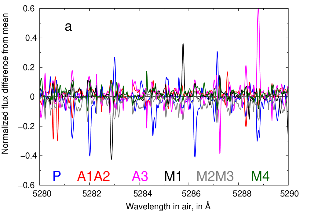
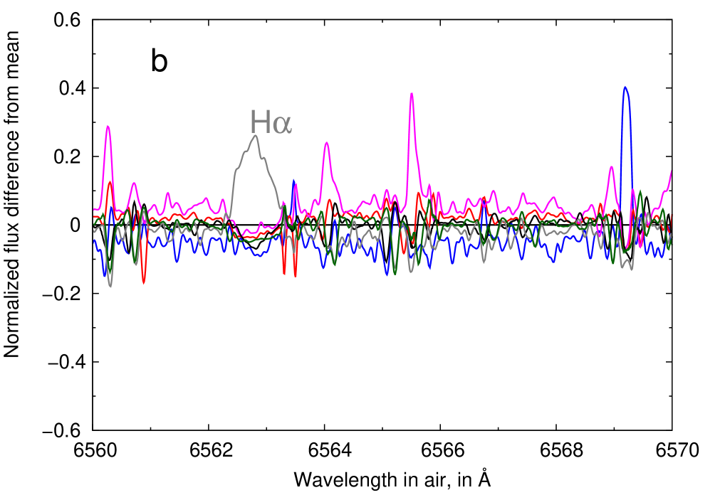
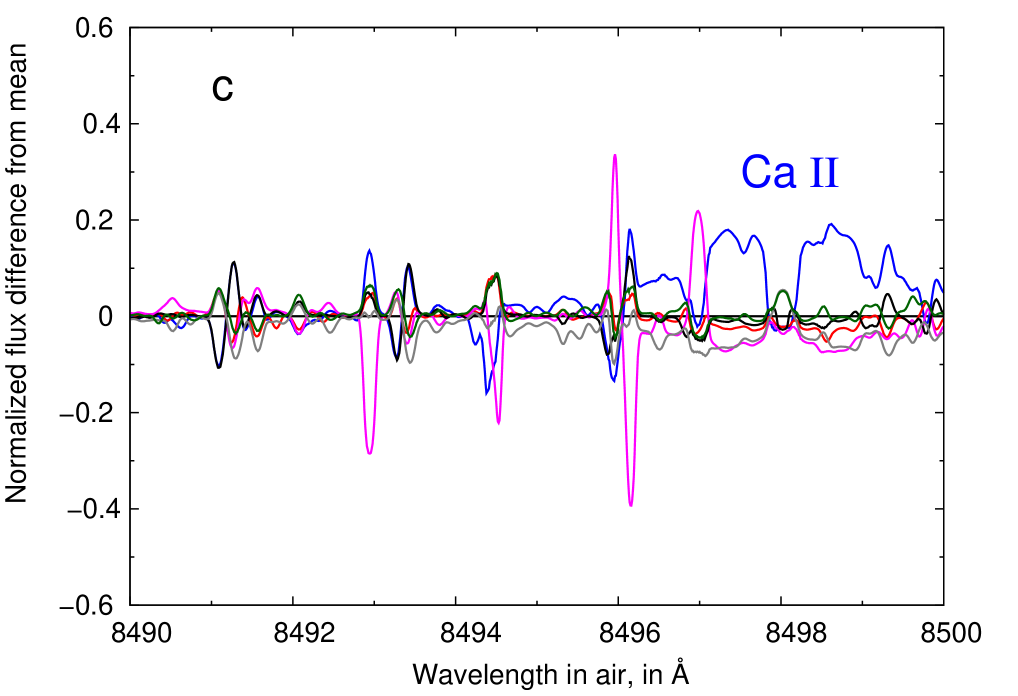
Figure 14: Normalized flux differences from the mean for six different models, for four different wavelength regions. The six model codes appear across the bottom of panel (a) in the colours used in the plots. (a) blue region with relatively low rms difference; (b) region containing H$\alpha$; (c) region containing the IR Ca II triplet 8498 Å line; (d) region with high rms difference due to differences in a strong Mg I line at 8807 Å.

5 Discussion

As pointed out above, there seems to be no obvious difference between the results from different ‘code-families’ (MARCS, ATLAS). Experiment 2, the ‘fixed parameter comparison’, revealed quite significant differences in the synthetic line strengths, in particular for some medium to weak lines, molecular lines, and for the Ca II IR triplet. The main reason for these differences seems to be the different line parameters used by the different groups. However, the spectrum modelling differences are only one aspect leading to the resulting scatter of the derived parameters of, e.g., Star 1. In the following we briefly discuss various aspects that may affect the result.

5.1 Method of parameter determination

In an ideal world, observations with their uncertainties would be combined with models and their uncertainties via a Bayesian approach to estimate stellar parameters, including correlations between parameters. This is especially difficult in the real world, because uncertainties are often difficult to estimate. Some of the observing parameters (e.g., spectral point-spread function, telluric correction) require complex models to determine uncertainties, and, to our knowledge, no modelling code currently propagates uncertainties in, e.g., oscillator strengths and pressure broadening coefficients through to wavelength-dependent uncertainties on the output spectra. Therefore, different groups tried different approaches to fitting what they regard as the most reliable parts of the spectra with differing weighting schemes.

The participating teams have chosen a remarkable variety of approaches for deriving the stellar parameters. The groups can be divided into those which measured equivalent widths from the provided spectra which they compared to calculated equivalent widths (A2, A5, T), and those which employed spectrum synthesis. The latter groups synthesized either continuous wavelength intervals (M2, M3a, M4, M5, A3, P, C), or intervals around selected spectral lines (M1, M3b, M6, A1, A4; see Fig. 1). The main difference between the two M3 analyses was in the characteristics of the spectra that were fed through an automated pipeline into the parameter determination code MATISSE. M3a was tailored to low resolution ($R\sim$6 500) spectra covering almost continuous wavelengths within a region of $\sim$300Å. M3b was applied to spectra at a higher resolution ($R\sim$15 000), using discontinuous wavelength regions totaling $\sim$435Å spread over $\sim$1800Å.

The M2, M5, M6, A1, A3, and T, analysis started by determining approximate stellar parameters (or at least one parameter) from a comparison of observed photometry and synthetic colours (see Tables 12 to 15, and Section 3.2.3). M1 used the colour information at a later step to partly lift the degeneracy between $T_{\rm eff}$/ $\log g$ and metallicity. The remaining groups did not use the provided colour information.

The experiment participants used different methods to calculate equivalent widths or synthetic spectra. A2 applied automatic measurement of equivalent widths from synthetic spectra calculated with SYNTHE, using fixed-width integration around the center of each spectral line. A5 used the plane-parallel code MOOG (original version described in Sneden 1973) to calculate the equivalent widths, while T employed the method described in Tsuji (1986). A1, A3, and A4 worked with the plane-parallel line-formation code SYNTHE (Kurucz 1993b) for spectrum synthesis. M1 used a spherically-symmetric spectrum synthesis code developed for the study of line profile variability in AGB stars, described in Nowotny et al. (2010, their Section 2.4). M2, M3, and M5 used the spectral line formation code TURBOSPECTRUM (Alvarez & Plez 1998), while M4 used the code BSYN developed in Uppsala. Both TURBOSPECTRUM and BSYN provide the option to compute the radiative transfer in spherically-symmetric geometry, and both have a number of subroutines in common with the MARCS code. M6 used the MOOG code in spectrum-synthesis mode. The P and C analyses employed the spectrum synthesis integrated in the PHOENIX and CODEX packages, respectively.

The methods used for parameter optimization with the provided spectra are briefly summarized as follows. M1, M2, M4, M5, A2, A3, P, and C based their fit on minimizing a weighted squared difference ($\chi^{2}$) between the observed and the synthetic spectrum, either for the whole wavelength range available or for selected regions containing parameter-sensitive features. Some of the groups complemented the automatic fit with an inspection by eye (M1, M2, M5). M3 used the MATISSE algorithm, which has been developed for fast automatic parameter determination of low- to high-resolution stellar spectra, and is based on a local multi-linear regression method (for details see Section 3.1.3). A1 verified by eye that the observed spectrum was reproduced by the model spectrum with the photometric $T_{\rm eff}$ values, and adjusted the $\log g$ and [Fe/H] values manually in order to fit selected features sensitive to these parameters. M6, A4, and A5 derived the stellar parameters by removing line abundance trends. This “classical” method effectively combines the information from spectrum points within spectral lines, and uses knowledge on spectral line behaviour to infer the parameters. The difference was that M6 and A4 used spectrum fits for each line, and A4 also fitted the wings of strong lines, while A5 worked with equivalent widths. In the T analysis, $T_{\rm eff}$ was derived from photometry, a fixed value was chosen for $\log g$, and the abundance analysis was performed as described in Tsuji (2008).

A prime issue that has to be discussed is how these different strategies affect the result. There are good reasons to start with photometry data to constrain the stellar parameters. Photometric colours have the advantage of providing information over a wide baseline in the spectrum. Some of them – of course depending on the spectral types of the target stars – are nearly independent of metallicity over a wide range of temperatures (for cool stars $V-K$ can be used very well), while others involve a dependence on surface gravity. A clear disadvantage, however, that can introduce considerable error for this approach, is interstellar reddening, although this will not play a significant role in the context of our experiment. Narrow-band photometry – e.g. using filters to study the strength of individual molecular bands (see e.g. Wing 2007) – may be a way to circumvent this weakness.

Furthermore, photometric colours are affected by the actual chemical composition of the star, especially for cool objects with altered C/O ratios (e.g. Star 4 in Experiment 1). In such cases, the uncertainty in the derived $T_{\rm eff}$ is expected to increase significantly. To make use of the photometry, a calibration relating colours and parameters is required, which can be either purely theoretical or semi-empirical. A considerable number of such calibrations have been published throughout the years. Thus, it is not surprising that each of the groups using the colour information in Experiment 1 applied a different calibration (see Tables 12 to 15). The resulting estimates for $T_{\rm eff}$ agree rather well, except for Star 4, as expected from the discussion above (see also discussion in Section 3.1.5). For $\log g$ and [Fe/H], the values disagree in the few applicable cases.

All of the methodologies used here for the parameter determination suffer from several sources of uncertainty. First, in the squared-difference minimization method, similar $\chi^{2}$ values can be obtained for a certain range of models, and so the “best parameters” must be constrained by additional considerations. An interesting aspect is that the groups using this method defined the difference measure ($\chi^{2}$) in different ways, in particular regarding the weight factor. It is not clear how this might affect the outcome of the analysis. Note that we did not compare individual $\chi^{2}$ values to assess the results from the different groups, as those will also depend on the length and location of the wavelength sections. Second, none of the methods provides a straight-forward way for estimating the uncertainties in the derived parameters, except for MATISSE (M3) which automatically provides error estimates based on the signal-to-noise ratio. Third, separating the effects of different line-broadening parameters such as micro- and macro-turbulence or rotation may be difficult in the case of the spectral synthesis method. On the other hand, the full spectrum fit can – in principle – better handle spectra with lots of blended lines, and it includes a large number of spectral indicators at once.

Since M2 and M3 used identical model spectra for their analysis, the differences in the results are entirely due to the different methods applied. In addition, the influence of different methods can be seen by comparing the M3a and M3b results. M2 and M3b both used the optical wavelength region (4900 – 6800 Å) for the fit, although slightly different subintervals were selected. Furthermore, M3b worked at decreased spectral resolution, while M2 used the full resolution. The resulting $T_{\rm eff}$ values are comparable for both $\alpha$ Tau and $\alpha$ Cet, while $\log g$ and [Fe/H] differ. This is in line with the findings of M4 that the optical region is mostly sensitive to $T_{\rm eff}$ variations. Hence, the “best-fit” values of $\log g$ and [Fe/H] will be rather arbitrary. Using only the RVS wavelength region (8470-8740 Å) and a low resolution, M3a gives different results for all three parameters. The $T_{\rm eff}$ values are higher for both benchmark stars (compared to M3b), while $\log g$ and [Fe/H] are higher for one star and lower for the other.

The P analysis for $\alpha$ Tau resulted in the highest value for $\log g$. This could be explained by low values of the pressure broadening parameters for strong atomic lines used by the P code, apparent in Fig. 14 c and d. To achieve a fit to broad observed line wings, the P analysis requires a higher $\log g$ value than the other models.

5.2 Limitations in accessible parameter range

Typically, models are optimized for application to a specific range of stellar parameters. In Experiment 1 we also see this in some limits of the tested parameter range. For example the CODEX code (C) has an upper limit in $\log g$ of 0.0, and thus the ‘best fit’ result in the case of Star 2 is naturally somewhat offset from the findings of the other groups.

As mentioned in Section 4.2, most participating groups explored only a small volume in parameter space around values estimated from photometry or comparisons with spectra of standard stars. Only M3 and A2 based the analysis of Star 1 and Star 2 on a large model grid, and they obtained results similar to the others, except for $T_{\rm eff}$ in the case of A2.

5.3 LTE and non-LTE

As one of the underlying assumptions in this comparative work, all the participants used LTE stellar model atmospheres with LTE line formation (except for the M6 Ca abundance analysis described below). A full non-LTE treatment of all elements in the atmospheres of cool giants is a very complex task that can not yet be achieved due to the lack of quantitative atomic data. Nevertheless, non-LTE theoretical models of giant stars have been computed by Short & Hauschildt (2005), taking into account the main electron contributors. They showed that non-LTE effects on the structure of the atmosphere increase with decreasing metallicity, especially deep and high up in the photosphere. The change in the structure will change the line formation domains and the intensity of the photospheric lines. Fortunately, the change in the structure seems to be negligible at solar metallicity. Thus, one can use LTE model atmospheres for a partial non-LTE analysis by applying line synthesis of a given element in non-LTE. This has been done by many authors, e.g., Thévenin & Idiart (1999); Shchukina & Trujillo Bueno (2001). More recently, Mashonkina et al. (2011) showed with a very complete model atom of Fe I/II that the non-LTE corrections do not exceed 0.1 dex for solar and mildly low metallicities.

The LTE assumption may strongly affect the surface gravity determination when this astrophysical parameter is constrained by the ionization equilibrium to follow Saha’s law. The surface gravity deduced from the photometry and evolutionary tracks is usually used as a starting point for spectroscopic iteration between two ionization stages of iron. This latter procedure relies on the assumption of LTE and tends to give LTE values of $T_{\rm eff}$ and $\log g$ smaller than those from photometric determinations. Therefore, this can also impact the iron abundance analysis. A temporary solution to this problem can be to trust the surface gravity given by the photometric estimation, and to use only Fe II lines, which are known to be free of non-LTE effects (see, e.g. Mashonkina et al. 2011), to determine [Fe/H]. An investigation of non-LTE effects on Fe line formation is not within the scope of the present paper. However, the M6 team determined the abundance of Ca in $\alpha$ Tau using non-LTE radiative transfer in an LTE model atmosphere, as described in the following paragraph.

Ca I/Ca II analysis of $\alpha$ Tau:

The M6 team aimed to find the same abundance for Ca I and Ca II. It was decided to compare the abundance determined using the IR triplet (8498, 8542, 8662) Å with the abundance determined using the optical triplet (6102, 6122, 6162) Å. A non-LTE analysis was performed, using a Ca I atom with 153 energy levels (taking into account fine structure), 2120 bound-bound radiative transitions and 11476 bound-bound collisional transitions with electrons, and 81 photoionization tables from TopBase. They used a Ca II model atom with 74 energy levels, 422 bound-bound radiative transitions, 2628 bound-bound collisional transitions with electrons, and 40 photoionization tables from TopBase. The contribution of inelastic collisions with neutral hydrogen was neglected due to the lack of accurate quantum-mechanical calculations to determine their importance, and the Stark effect in the line-broadening parameters was also neglected (see Merle et al. 2011). Spherical MARCS model atmospheres with standard composition were adopted. The code MULTI2.2, slightly modified for the collisional transition part, solves the radiative transfer and statistical equilibrium equations consistently and computes line profiles, equivalent widths and contribution functions for all the radiative transitions. They performed several computations for the model atmosphere 4000/1/0 ($T_{\rm eff}$/$\log g$/[Fe/H]) with different calcium abundances for Ca I and Ca II and decided by eye the best metallicity fitting both the Ca I lines and the Ca II triplet lines. This turns out to be [Ca/Fe] = $-0.3\pm 0.1$ with an adopted [Fe/H]=0.0 (see Table 12). We note that the core of the Ca II IR lines is still poorly reproduced, because of the existence of a chromosphere where the line cores form (see Berio et al. 2011).

5.4 Geometry

In addition to $T_{\rm eff}$, $\log g$ and abundances, stellar spectra are in principle also affected by the extension of the atmosphere, which can be parameterized by ($T_{\rm eff}$/5770)$(R/{\rm R}_{\odot})(M/{\rm M}_{\odot})^{-1}$. If the atmospheric extension could be modelled from spectra, then this would uniquely constrain $M$, $L$ and distance independently of evolutionary models. None of the models submitted in the study of stars 1 through 4 came up with a meaningful constraint on extension, but this by itself does not mean it is insignificant.

Especially extended atmospheres can show very strong effects of extension such as molecular shells, where it is not even obvious if a strong line in a cool extended shell will appear in absorption or emission, Ohnaka (e.g. 2004). Extreme effects observed in highly evolved stars are difficult to model completely in studies such as this paper, because they necessarily require departures from hydrostatic equilibrium (e.g. pulsation and shocks) in order to elevate the material. The effects in stars with only low-amplitude oscillations such as Star 2 are much smaller, but are significant enough that many modelling teams chose to use spherical codes. This mirrors the experience of the various groups that even in a purely hydrostatic world the sphericity effects on spectra increase towards cooler giants.

The extension of an atmospheric model is typically parameterised by a single statement: whether the model is spherical (with a reasonable value of extension) or plane-parallel. For $T_{\rm eff}$ greater than 4000 K, Heiter & Eriksson (2006) show typical abundance differences between spherical and plane-parallel codes of 0.1 dex. This is comparable to or smaller than the metallicity errors estimated from models in this paper, but suggests that if sphericity is not taken into account, the atmospheric parameters will be mis-estimated. We suggest that further work on this topic is required, informed by detailed observations of a range of stars with well-known parameters and a range of atmospheric extensions.

5.5 Atomic and molecular line data

Accuracy and completeness of atomic and molecular data play a key role in fitting observed spectra with synthetic ones. In the experiments presented in this article we find various approaches to the compilation of input data. All MARCS-based analyses relied on atomic data extracted from the VALD database (in 2008–2009), while all ATLAS-based analyses used atomic data from the Kurucz web site. A few groups calibrated the $gf$-values on high-resolution spectra of standard stars – M3a and M5 on the Sun and Arcturus, and A4 on several standard stars, including the Sun, Arcturus, and $\mu$ Leo. A2 verified the atomic line data for the cases of the Sun and Procyon. Molecular data were included in all calculations except for M6 and A5. Typically, line lists for 8–11 different species were included. In the case of M2, M3, and M4, the data stem from the same sources (described in Gustafsson et al. 2008). For M1, the data sources are given in Lederer & Aringer (2009), and for M5 they are specified in Section 3.1.5. A1, A2, A3, A4, P, and C obtained molecular line data from the same sources (via the Kurucz website), see respective subsections of Section 3 for details. Data sources for T are given in Tsuji (2008).

The VALD database for atomic lines was therefore the prime source of atomic data, although the line lists have been extracted from different versions of the database. Sources for molecular line lists are less homogeneous, and also the number of molecules included varies from group to group. All line lists, both for atoms and for molecules, still require significant improvement. A way around missing line data is offered by the use of astrophysical oscillator strengths.

However, the derivation of astrophysical $gf$-values requires a reference object, for which atmospheric parameters and element abundances are known precisely. Currently, this is only the case for the Sun (even in that case some uncertainties remain). As the nature and strength of spectral lines appearing in the object under study (e.g. a cool giant) and the Sun will differ significantly, the astrophysical $gf$-values will be in most cases of limited use.

A possible approach would be to work differentially using a “chain” of reference stars, starting from parameters close to solar and leading towards the required area in parameter space. We assume that for each neighbouring pair of stars it will be possible to define a common set of spectral lines. The line data calibrated on the star “closer” to the Sun will then define the element abundances of the “new” star. However, astrophysical $gf$-values will always remain an unsatisfying solution. Good experimental data are certainly highly desired.

We note that oscillator strengths are only one element of the line data set required for each transition. Various damping constants used to parametrize collisional processes are equally important and equally uncertain. Differential work can remedy these uncertainties to a certain extent, in a similar way as for $gf$-values. For certain transitions, specialised theories are available, as for example for the hydrogen lines, but these are not implemented in all codes.

5.6 Convection

An important physical process to be included in the calculation of model stellar atmospheres is convection. The main effects of convection are 1) the contribution of the convective flux to the energy transport, leading to a modified temperature distribution compared to the purely radiative case; and 2) the generation of horizontal and vertical velocity fields, which modify the positions and shapes of spectral lines. The efficiency of convective energy transport and its effect on the temperature structure in the line-forming region depends on all three atmospheric parameters ($T_{\rm eff}$, $\log g$, [M/H]) in a complex way (the contribution of the convective flux to the total flux is shown e.g. in Fig. 4 in Heiter et al. 2002). At $T_{\rm eff}$$\approx$4000 K, the efficiency of convection reaches a maximum and seems to be independent of gravity or metallicity.

In all of the atmospheric models used for the experiments described in the present paper, the first effect of convection is included in an approximative way, based on the mixing length theory (MLT, Böhm-Vitense 1958). The practical implementation of the MLT varies somewhat between the different codes. In the ATLAS models, MLT convection is implemented as described in Kurucz (1970) and Castelli (1996), similar to the formulation according to Mihalas (1978). A variant of the latter is used in the PHOENIX models (Ludwig et al. 2002). In the MARCS models, the MLT formulation of Henyey et al. (1965) is used. This variation in the implementation results in different numbers of free parameters, and different meanings of these parameters, for each model, hampering a direct comparison (see Section 5.3.1 in Ludwig et al. 2002 for a discussion on the importance of the MLT formulation).

The free parameter dominating any discussion of MLT convection is the “mixing length,” i.e. the distance which convective elements can travel before they dissolve. It is usually specified in terms of the local pressure scale height, and typical values are between 0.5 and 3, depending on stellar parameters and whether spectral features or global stellar parameters are modelled. However, a number of additional parameters have to be set. The size of convective elements is usually assumed to be a single value and equal to the mixing length. The need for this “one-eddy” approximation is overcome in the alternative “full-spectrum-turbulence” convection models (e.g. Canuto & Mazzitelli 1991), where the distribution of kinetic energy generated by convection over different spatial scales is computed from a turbulence model. This treatment of convection has been implemented in ATLAS models by Heiter et al. (2002) and was compared to MLT models for $T_{\rm eff}$$\geq$4000 K, $\log g$$\geq$2 and a range of metallicities, but has not been used by any of the groups in the present paper. Additional free parameters are needed to specify the geometry of the convective elements and the temperature distribution within them. This determines the energy lost by radiation and thus the efficiency of convection. Furthermore, viscous energy dissipation is parametrized by a coefficient in the equation for the convective flux. The default values for these parameters are different in the ATLAS and MARCS models. However, since all free parameters basically are scaling factors in a single equation, this may be compensated by using different values for the mixing length.

An additional degree of freedom is provided in the MLT implementation of ATLAS models through the “overshooting option.” A smoothing procedure allows for a positive convective flux in stable layers next to the convection zone. Castelli et al. (1997) investigated the effect of this option for $T_{\rm eff}$$\geq$4000 K, $\log g$$\geq$2.5 and a range of metallicities. Comparison with observation indicated that except for the Sun, the atmospheric parameters derived with different methods were more consistent when the overshooting option was switched off.

The second effect of convection, the three-dimensional velocity field, is not treated at all by MLT. Additional Doppler broadening of spectral lines caused by convective motions is taken into account in the one-dimensional models by specifying the ad-hoc parameters micro- and macroturbulence (in units of velocity, see modelling descriptions in Section 3 and Tables 12 to 15).

Realistic modelling of the effects of surface convection on stellar spectra can only be achieved with time-dependent, three-dimensional, radiation-hydrodynamic numerical simulations (hereafter referred to as “3D models”). Such simulations have been done for the Sun for several decades, and have become increasingly accurate. This has been demonstrated by comparison to a variety of observations, not the least the profiles of numerous individual resolved spectral lines. Without applying any micro- or macroturbulence parameters, the wavelength shifts and asymmetries of the solar line profiles are in general very well reproduced (see, e.g., the detailed review by Nordlund et al. 2009).

3D surface convection models and spectra for stars other than the Sun are not yet widely available, due to the large amount of computing power and human post-processing time required. However, individual regions in the parameter space have been investigated thoroughly. The most relevant study in the context of this paper is that by Collet et al. (2007), who examined the effects of convection on spectral lines for red giant stars with $\log g$ = 2.2 at two different effective temperatures and [Fe/H] = $0,-1,-2,-3$. The largest effects when compared to 1D model atmospheres where found at the lowest metallicities, while the effects were minor at solar metallicity (abundance differences of up to 0.8 dex and within $\pm$0.1 dex, respectively). However, these models were significantly hotter and at lower $\log g$ than the stars investigated in the present paper.

The situation may improve rapidly in the near future, as at least two groups are computing larger grids of 3D models, using two different simulation codes. The “CIFIST grid” (Ludwig et al. 2009) and the “StaggerGrid” (Collet et al. 2011) both will include on the order of 100 models for main-sequence and red giant stars (25–30 $T_{\rm eff}$/$\log g$ combinations and four metallicities). Within the latter project, average temperature structures calculated from the full 3D models will be made publicly available, as well as corresponding values for micro- and macroturbulence for implementation with classical line-formation codes. This will be the first step towards a more realistic spectrum analysis of a variety of stars. We note that the parameters of the two benchmark stars $\alpha$ Tau and $\alpha$ Cet lie just outside of the parameter ranges investigated for convection effects so far, both in grids of 1D models and in sets of 3D models. However, both of the future 3D grids include a solar-metallicity model at ($T_{\rm eff}$, $\log g$) = (4000 K, 1.5), which should be close enough for establishing the importance of convection for spectrum modelling for these stars.

Finally, we point out that the spatial extension of hydrodynamic simulations can be set up in two different ways. In the surface gravity domain of red giants, the “box-in-a-star” approach is applicable (cf the two model grids mentioned above). In this approach, the simulation is performed for a box inside the stellar atmosphere, covering several convective cells. The horizontal boundaries of the box are periodic, the vertical boundaries are open, and the extensions of the box are small compared to the stellar radius. However, the characteristic size of the convective cells scales with pressure scale height and thus increases with decreasing gravity. In the extreme case of red supergiants such as Betelgeuse, the atmosphere contains only a few giant convective cells, and hydrodynamic simulations of the “star-in-a-box” type must be employed (Freytag et al. 2002). $\alpha$ Tau and $\alpha$ Cet lie in the transition region between these two approaches (close to $\log g$ = 1, Chiavassa et al. 2011). Since the influence of convection on spectrum modelling has not been investigated in this region so far, these two stars are very interesting test objects for future studies (see, however, Section 3.5 in Kučinskas et al. 2005 for a 3D hydrodynamical model and convection-related effects on colours of a late-type giant).

5.7 Other issues

An often neglected fact is that model atmosphere and synthetic spectrum codes rely on a wealth of physical input data besides the spectral line data discussed in Section 5.5. Apart from parameters describing convective processes, an example for these are data used for chemical equilibrium calculations (establishing the equation of state), namely partition functions and molecular dissociation energies. Another important ingredient are data describing bound-free and free-free transitions providing the continuous opacity. Although widely used standard references exist for much of these data (e.g. the “Kurucz routines” for continuous opacities, or Irwin 1981 for partition functions), these are evolving slowly and often are not described in detail. These “hidden data” leave room for differences of unknown degree between codes from different authors. Furthermore, they can lead to inconsistencies between model atmospheres and spectral synthesis. In this regard, the first step towards consistent spectrum modelling is to use spectrum synthesis and model atmosphere codes developed by the same author or group.

For example, the MARCS model atmosphere code and the BSYN synthetic spectrum code share many subroutines (e.g. for the chemical equilibrium) and the computation of the continuous opacities is consistent in both codes. The same is true for MARCS and TURBOSPECTRUM, and the “Kurucz suite” consisting of ATLAS9, ATLAS12, and SYNTHE.

6 Conclusions

Estimating stellar parameters by comparison of observed and synthetic spectra is always affected by inaccuracies in line data and assumptions of model stellar atmospheres for cool stars (cf. the extensive discussion of this issue in the context of cool, evolved giants by Gustafsson 2007). Due to these limitations even a ‘perfect’ fit of a spectrum cannot be seen as proof for a perfect model. We stress that it is not the intention of this paper to rank the various existing models of stellar atmospheres, but to learn from the effects caused by their differences.

Experiment 1 clearly illustrates the need to be cautious when comparing or combining stellar parameters that were derived using different model atmospheres and fitting strategies. We tried to illuminate various possible influences, but a clear trend in terms of a systematically higher or lower value for some parameter for a given assumption could not be derived. This is a very complex problem with various aspects that seem to partly compensate for each other.

It would be desirable to repeat the experiment using different modelling codes, but exactly the same method (e.g. a chi-square fit to preselected wavelength regions). Also, differences in atomic and molecular line lists should be sorted out. It seems to be extremely difficult to implement the use of equal input line data in the various codes, simply because of different requirements for the data format. This annoying obstacle could possibly be mitigated in the future by the use of a common infrastructure for atomic and molecular line data. An attempt to create such an infrastructure is currently underway in the VAMDC EU project (Dubernet et al. 2010). Finally, repeating the experiment using exactly the same tools may give a clearer idea about the reasons for different results between different codes.

One could ask whether the data given for Experiment 1 are sufficient to derive a unique set of parameters. No doubt additional data would set further constraints and resolve one or another degeneracy. A more extensive analysis of the existing data may produce some progress as well, but in our view it will be always limited by the accuracy of the line data and inaccuracies in our models, which definitely require further attention in the future.

However, we think that Experiment 1 represents quite a typical situation in observational astrophysics: a piece of the spectrum and some photometric data are given, and some fixed strategy to analyze the data is adopted. With our limited experiment we want to point out that the atmospheric model and the analysis method used can have a significant effect on the absolute values of the derived stellar parameters. Bringing together such a variety of groups fitting stellar spectra by the use of various methods, this paper provides also an unprecedented snapshot of the current status of this field.

For future analysis projects, we recommend working differentially as far as possible. For stellar samples with parameters significantly different from the Sun, a set of suitable benchmark stars may serve as stepping stones for a piecewise differential analysis.