Microscopic description of quadrupole-octupole coupling in Sm and Gd isotopes with the Gogny Energy Density Functional.

Abstract

The interplay between the collective dynamics of the quadrupole and octupole deformation degree of freedom is discussed in a series of Sm and Gd isotopes both at the mean field level and beyond, including parity symmetry restoration and configuration mixing. Physical properties like negative parity excitation energies, E1 and E3 transition probabilities are discussed and compared to experimental data. Other relevant intrinsic quantities like dipole moments, ground state quadrupole moments or correlation energies associated to symmetry restoration and configuration mixing are discussed. For the considered isotopes, the quadrupole-octupole coupling is found to be weak and most of the properties of negative parity states can be described in terms of the octupole degree of freedom alone.

I Introduction.

The nuclear mass region with proton number $Z\approx 60$ and neutron number $N\approx 90$ is receiving at present much attention, both experimental and theoretically, since it is a region where nuclear structure collective effects of different nature overlap butler_96 . Particularly interesting in this context is the interplay between quadrupole transitional properties in $N\approx 90$ isotones and octupole deformation manifestations in nuclei with proton $Z\approx 56$ and neutron $N\approx 88$ numbers. On one hand, isotones with $N\approx 90$ have been found as empirical realizations exp_x5 of the critical point symmetry $X(5)$, introduced iachello to describe analytically the first order phase transition from spherical $[U(5)]$ to well deformed $[SU(3)]$ nuclei. Such critical point symmetries, have recently been studied within various microscopic approaches, either relativistic or non-relativistic (see, for example, ring_x5 ; ours_x5_1 ; ours_x5_2 ; Egido-Tomas-Nd and references therein).

On the other hand, it is well known butler_96 that there is a tendency towards octupolarity around particular neutron/proton numbers, namely $N/Z=$ 34, 56, 88 and 134. The emergence of octupolarity in these nuclear systems can be traced back to the structure of the corresponding single-particle spectra which exhibit maximum coupling between states of opposite parity, where the $(N+1,l+3,j+3)$ intruder orbitals interact with the $(N,l,j)$ normal-parity states through the octupole component of the effective nuclear Hamiltonian. When the mixing is strong enough, the nucleus displays an octupole deformed ground state butler_96 . In particular, for nuclei with $Z\approx 56$ ($N\approx 88$) the coupling between the proton (neutron) single-particle states $h_{11/2}$ ($i_{13/2}$) and $d_{5/2}$ ($f_{7/2}$) has been considered as mainly responsible for mean field ground state octupolarity.

Figure 1: MFPESs computed with the Gogny-D1S EDF in panel a) and Gogny-D1M EDF in panel b) for the nucleus ¹⁵⁰Sm. Taking the lowest energy as a reference, the contour lines extend from 0.25 MeV up to 4 MeV in steps of 0.25 MeV. Full, long dashed and short dashed contours are used successively to help identify contours more easily. Dotted lines correspond to contours starting at 5 MeV and extending to 8 MeV in steps of 1 MeV.

The search for signatures of stable octupole deformations in atomic nuclei has been actively pursued during the last decades butler_96 ; aberg_90 . As a main feature, octupole deformed even-even nuclei display particularly low-lying negative-parity $1^{-}$ states. In the case of stable octupole deformations, the $0^{+}$ and $1^{-}$ states represent the members of parity doublets, giving rise to alternating-parity rotational bands with enhanced $E1$ transitions among them. These fingerprints of octupole deformations have already been found in the particular regions mentioned above, but especially in the rare-earth and actinide regions butler_96 ; aberg_90 .

For the sample of nuclei considered in the present study (i.e., ^146-154Sm and ^148-156Gd), experimental fingerprints have been obtained through the observation of octupole correlations at medium spins, as well as the crossing of the octupole and the ground state band, pointing to the fact that reflection symmetric and asymmetric structures coexist in ¹⁵⁰Sm urban_87 and ¹⁴⁸Sm urban_91 . A recent study garrett_09 has analyzed the lowest four negative-parity bands in ¹⁵²Sm and has found an emerging pattern of repeating excitations, built on the $0^{+}_{2}$ level and similar to that of the ground state, suggesting a complex shape coexistence in ¹⁵²Sm.

The experimental findings urban_87 ; urban_91 ; garrett_09 mentioned above, already suggest that it is timely and necessary to carry out systematic studies of the quadrupole-octupole interplay in this and other regions of the nuclear chart, starting from modern (global) relativistic PR-VE-RI-2005 ; review-Bender and/or non-relativistic review-Bender ; gogny ; gogny-d1s ; bal08 nuclear Energy Density Functionals (EDFs), with reasonable predictive power all over the nuclear chart.

Let us remark that the microscopic study of the dynamical (i.e., beyond mean field) quadrupole-octupole coupling in the considered Sm and Gd isotopes is also required to better understand the extent to which a picture of independent quadrupole and octupole excitations persists or breaks down for nuclei with neutron number $N\approx 88$. This, together with the available experimental fingerprints urban_87 ; urban_91 ; garrett_09 for octupolarity in the region, is one of the main reasons driving our choice of the nuclei ^146-154Sm and ^148-156Gd as a representative sample to test the performance of the different approximations and EDFs considered in the present study.

Table 1: Proton $E_{p}(Z)$ (MeV) and neutron $E_{p}(N)$ (MeV) pairing energies, dipole $D_{0}$ (efm) moment, quadrupole $Q_{20}$(b) and octupole $Q_{30}$(b^3/2) moments at the minima of the MFPESs for the isotopes ^146-154Sm. Results are given for both Gogny-D1S and Gogny-D1M EDFs.

Nucleus		$E_{p}(Z)$	$E_{p}(N)$	$D_{0}$	$Q_{20}$	$Q_{30}$			$E_{p}(Z)$	$E_{p}(N)$	$D_{0}$	$Q_{20}$	$Q_{30}$
		D1S						D1M
146Sm		-14.64	-3.58	0.00	1.20	0.00			-15.67	-5.20	0.00	0.60	0.00
148Sm		-12.41	-3.34	0.18	3.00	1.25			-13.92	-4.52	0.14	3.00	0.75
150Sm		-10.98	-1.53	0.41	4.80	1.50			-11.80	-2.99	0.35	4.80	1.25
152Sm		-6.58	-5.57	0.00	7.20	0.00			-8.24	-6.18	0.00	6.60	0.00
154Sm		-5.91	-3.27	0.00	7.80	0.00			-6.38	-4.63	0.00	7.80	0.00

From a theoretical perspective, many different models have been used to describe octupole correlations in atomic nuclei. For a detailed survey the reader is referred, for example, to Ref. butler_96 . Calculations based on the shell-correction approach with folded Yukawa deformed potentials moller_81 ; leander_82 , as well as calculations based on Woods-Saxon potentials with various models for the microscopic and macroscopic terms naza_84 ; naza_92 , predicted a significant stabilization of octupole deformation effects in various nuclear mass regions. Pioneer Skyrme-HF+BCS calculations including the octupole constraint and restoring parity symmetry were carried out in Ref. mar83 . Subsequent calculations in Ref. bon86 included both quadrupole and octupole constraints at the same time but at the mean field level only. On the other hand, microscopic studies of octupole correlations with Skyrme and Gogny EDFs, both at the mean field level and beyond with different levels of complexity, have already been reported (see, Refs. bon88 ; bon91 ; hee94 ; mey95 ; rob87 ; rob88 ; egi90 ; egi91 ; gar98 ; egi92 ; rob10 and references therein) for several regions of the nuclear chart. Theoretical studies in the Sm region include mean field based calculations with the collective hamiltonian and the Gogny force egi92 , the IBM study with $spdf$ bosons of Ref. babilon_05 or the collective models using a coherent coupling between quadrupole and octupole modes minkov_06 and new parametrizations of the quadrupole and octupole modes bizzeti_10 . Non-axial pear-like shapes in this region were considered, for example, in Refs. skalski_91 . Additionally, the isotopes ^146-156Sm have been investigated very recently within the constrained reflection-asymmetric relativistic mean field (RMF) approach zhang_10 based on the parametrization PK1 RMF-PK1 for the RMF Lagrangian together with a constant gap BCS approximation for pairing correlations.

In the present work, we investigate the interplay between octupole and quadrupole degrees of freedom in the sample of nuclei ^146-154Sm and ^148-156Gd. We use three different levels of approximation. First, the constrained (reflection-asymmetric) Hartree-Fock-Bogoliubov (HFB) framework is used as starting point providing energy contour plots in terms of the (axially symmetric) quadrupole $Q_{20}=\langle{\Phi}|\hat{Q}_{20}|{\Phi}\rangle$ and octupole $Q_{30}=\langle{\Phi}|\hat{Q}_{30}|{\Phi}\rangle$ moments (where $|{\Phi}\rangle$ is the corresponding HFB intrinsic wave function). Within this mean field framework we pay attention to the shape changes in the considered nuclei and their relation with the underlying single-particle spectrum butler_96 ; rob10 ; ours-PT .

As will be discussed later on, the $(Q_{20},Q_{30})$ mean field potential energy surfaces (MFPES) obtained for the nuclei ^146-154Sm and ^148-156Gd are, in most of the cases, very soft along the $Q_{30}$ direction indicating that the (static) mean field picture is not enough and that a (dynamical) beyond mean field treatment is required. Therefore, both the minimization of the energies obtained after parity projection of the intrinsic states mar83 ; egi91 ; egi92 as well as quadrupole-octupole configuration mixing calculations in the spirit of the Generator Coordinate Method (GCM) rs , are subsequently carried out. The analysis of the two sets of results allows to disentangle the role played in the dynamics of the considered nuclei by the restoration of the broken reflection symmetry and the fluctuations in the ($Q_{20}$,$Q_{30}$) collective coordinates. Similar calculations with the Skyrme functional where carried out in Ref mey95 for a lead isotope.

Table 2: The same as Table I but for the isotopes ^148-156Gd.

Nucleus		$E_{p}(Z)$	$E_{p}(N)$	$D_{0}$	$Q_{20}$	$Q_{30}$			$E_{p}(Z)$	$E_{p}(N)$	$D_{0}$	$Q_{20}$	$Q_{30}$
		D1S						D1M
148Gd		-15.22	-4.27	0.00	0.66	0.00			-16.11	-5.35	0.00	0.00	0.00
150Gd		-14.22	-3.63	0.19	3.60	0.75			-15.43	-5.03	0.05	3.00	0.25
152Gd		-12.69	-3.02	0.27	4.80	1.00			-13.18	-4.76	0.15	4.80	0.50
154Gd		-7.63	-6.26	0.00	7.20	0.00			-9.25	-6.88	0.00	6.60	0.00
156Gd		-7.18	-4.86	0.00	7.80	0.00			-7.66	-6.20	0.00	7.80	0.00

To the best of our knowledge, the hierarchy of approximations (i.e., reflection-asymmetric HFB, parity projection and $(Q_{20},Q_{30})$-GCM) considered in the present work belong, at least for the case of the Gogny-EDF, to the class of unique and state-of-the-art tools for the microscopic description of quadrupole-octupole correlations in atomic nuclei. Let us also stress that, the two-dimensional GCM (2D-GCM) framework used in the present study represents an extension of the treatment of octupolarity reported in Refs. rob10 ; egi92 , where a one-dimensional collective hamiltonian based on several approximations and parameters extracted from $Q_{30}$-constrained HFB calculations, was considered. Here, on the other hand, the octupole and quadrupole degrees of freedom are explored simultaneously and the kernels involved in the solution of the corresponding Hill-Wheeler equation rs are computed without assuming a gaussian behavior of the norm overlap neither a (second order) expansion over the non-locality of the hamiltonian kernel. Therefore, the present study for the selected set of Sm and Gd nuclei, to the best of our knowledge the first of this kind for the case of the Gogny-EDF, may also be regarded as a proof of principle concerning the feasibility of the calculations to be discussed later on. Pioneer calculations along the same lines considered in the present study, but based on the Skyrme-EDF, have been carried out in Ref. mey95 ; Heenen.01 .

Figure 2: In panel a) the reflection symmetric (i.e., $Q_{30}$=0) MFPECs for ^146-154Sm and in panel b) for ^148-156Gd are plotted as functions of the axially symmetric quadrupole moment $Q_{20}$. Results for both Gogny-D1S with full line and Gogny-D1M with dashed line are given. In each panel the energies are referred to the D1S ground state energy of the heavier isotope.

In addition to the standard Gogny-D1S gogny-d1s parametrization, which is taken as a reference, the D1M parametrization gogny-d1m will also be considered. The functional Gogny-D1S has a long standing tradition and it has been able to describe many low-energy experimental data all over the nuclear chart with reasonable predictive power both at the mean field level and beyond (see, for example, Refs. gogny-d1s ; rob87 ; rob88 ; egi90 ; egi91 ; gar98 ; rod02 ; egi04 ; egi04b ; gogny-other-1 ; gogny-other-2 ; gogny-other-5 ; bertsch ; peru ; hilaire ; delaroche10 ; PLB-2010-rayner and references therein). On the other hand, the D1M parametrization gogny-d1m that was tailored to provide a better description of masses is now proving its merits in nuclear structure studies not only in even-even nuclei ours-PT ; gogny-d1m ; ours2 ; PLB-2010-rayner ; ours-SrZrMo-quasi ; ours-Rb-quasi ; ours-Y-Nb-quasi , but also in odd nuclei in the framework of the Equal Filling Approximation (EFA) PLB-2010-rayner ; ours-SrZrMo-quasi ; ours-Rb-quasi ; ours-Y-Nb-quasi . In this paper the results of both D1S and D1M are compared to verify the robustness of our predictions with respect to the particular version of the interaction and to test the performance of D1M in the present context of quadrupole-octupole coupling.

The paper is organized as follows. In Secs. II, III and IV we briefly describe the theoretical formalisms used in the present work and subsequently the results obtained with them. Mean field calculations will be discussed in Sec. II. Parity projection and configuration mixing results will be presented in Secs. III and IV, respectively. In particular, in Sec. IV especial attention will be paid to beyond mean field properties in the considered nuclei -dynamical octupole and dipole moments, correlation energies, reduced transition probabilities B(E1) and B(E3) as well as energy splittings- and their comparison with available experimental data. Finally, Sec. V is devoted to the concluding remarks and work perspectives.

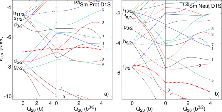
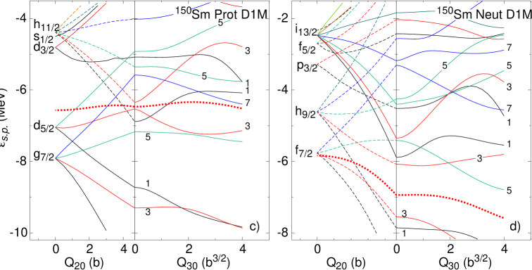
Figure 3: (Color online) Single particle energies (see text for details) in ¹⁵⁰Sm are plotted as a function of the quadrupole moment $Q_{20}$ (in barn) up to the value corresponding to the ground state minimum. From there on, the plot continues with the representation of the SPEs as a function of the octupole moment $Q_{30}$. In the part of the plot where the SPEs are plotted versus $Q_{20}$, full (dashed) curves stand for positive (negative) parity levels. The thick (red) dashed line in each plot represents the chemical potential. In the part of the plot where the SPEs are plotted versus $Q_{30}$ some levels around the Fermi level are labeled with twice their $J_{z}$ value. Panels a) and b) (c) and d)) correspond to results obtained with D1S (D1M) EDFs. Panels a) and c) (b) and d)) correspond to protons (neutrons).

II Mean field systematics.

The aim of the present work is the study of the quadrupole-octupole dynamics in selected Sm and Gd isotopes with neutron number 84 $\leq$ N $\leq$ 92. Three different levels of approximation are considered: the HFB method with constraints in the relevant degrees of freedom, parity projection (with minimization of the energy after projection) and the Generator Coordinate Method (GCM) with $Q_{20}$ and $Q_{30}$ as collective coordinates. For a detailed survey on the three techniques the reader is referred to Ref. rs . The Gogny EDF is used consistently in the three methods both with the D1S and D1M parametrizations.

First, $(Q_{20},Q_{30})$-constrained HFB calculations are performed for the nuclei ^146-154Sm and ^148-156Gd to obtain a set of states $|\Phi({\bf Q})\rangle$ labeled by their corresponding multipole moments ${\bf Q}=(Q_{20},Q_{30})$. The $K=0$ quadrupole $Q_{20}$ and octupole $Q_{30}$ moments are given by the average values

$$Q_{20}=\langle\Phi|z^{2}-\frac{1}{2}\left(x^{2}+y^{2}\right)|\Phi\rangle,$$ (1)

and

$$Q_{30}=\langle\Phi|z^{3}-\frac{3}{2}\left(x^{2}+y^{2}\right)z|\Phi\rangle.$$ (2)

Axial and time reversal are self-consistent symmetries in the mean field calculations. As a consequence of the axial symmetry imposed on the HFB wave functions $|{\Phi}\rangle$, the mean values of the multipole operators $\hat{Q}_{2\mu}$ and $\hat{Q}_{3\mu}$ with $\mu\neq 0$ are zero by construction. Aside from the constraints on the quadrupole and octupole moments, a constraint on the center of mass operator is used to place it at the origin of coordinates in order to prevent spurious effects associated to center of mass motion. The HFB quasiparticle operators $(\hat{\alpha}_{k}^{\dagger},\hat{\alpha}_{k})$ rs have been expanded in an axially symmetric harmonic oscillator (HO) basis $(\hat{c}_{l}^{\dagger},\hat{c}_{l})$ containing 13 major shells as to grant convergence for all the observable quantities. For the solution of the HFB equation, an approximate second order gradient method rob11 is used.

The MFPES have been computed in a grid with $Q_{20}$ in the range from -30b to 30b in steps of 0.6 b and the octupole moment $Q_{30}$ in the range from 0 b^3/2 to 3.75 b ^3/2 in steps of 0.25 b^3/2. Negative values of the octupole moment are not computed explicitly as the corresponding wave function can be obtained from the positive $Q_{30}$ one by applying the parity operator. As the Gogny EDF is invariant under parity (see rod02 ; egi04 for a discussion of the meaning of symmetry invariance for density dependent ”forces”) the energy has the property $E_{HFB}(Q_{20},Q_{30})=E_{HFB}(Q_{20},-Q_{30})$ and therefore is an even function of the octupole moment. For this reason, in the graphical representation of the PES only positive values of $Q_{30}$ are considered.

Figure 4: Positive $\pi$=+1 (upper panels) and negative $\pi$=-1 (lower panels) parity-projected potential energy surfaces (PPPES) computed with the Gogny-D1S (left panel) and Gogny-D1M (right panel) EDFs for the nucleus ¹⁵⁰Sm. See caption of Fig 1 for the contour line patterns.

The MFPESs obtained for the nucleus ¹⁵⁰Sm, with the parametrizations D1S and D1M of the Gogny-EDF, are shown in Fig. 1 as an illustrative example of our mean field results. For the sake of presentation, quadrupole and octupole moments have been constrained in the plots to the ranges -10 b $\leq Q_{20}\leq$ 20 b and 0 b^3/2 $\leq Q_{30}\leq$ 3.75 b^3/2, respectively. The similitude between the D1S and D1M results both in the $Q_{20}$ and $Q_{30}$ directions is remarkable. In previous calculations in other regions and looking at different physical effects ours-PT ; PLB-2010-rayner ; ours-SrZrMo-quasi ; ours-Rb-quasi ; ours-Y-Nb-quasi we have already noticed the same similitude between D1S and D1M results. Focusing on the MFPES, the absolute minimum is located in the prolate side at a finite value of the octupole moment. The minimum is very shallow along the $Q_{30}$ direction. Another minimum is observed in the oblate side, but this time centered at $Q_{30}=0$. For the other nuclei considered the energies look similar and therefore they are not shown. The most relevant mean field quantities for the ground states are summarized in Tables I and II. In order to better understand the quadrupole deformation properties of the studied nuclei, the reflection symmetric (i.e., $Q_{30}$=0) mean field potential energy curves (MFPECs) are depicted for all the considered nuclei in Fig. 2. A transition from weakly deformed ground states in the N=84 nuclei ¹⁴⁶Sm and ¹⁴⁸Gd to well (quadrupole) deformed ground states in ^152,154Sm and ^154,156Gd (prolate moments 6.6 b $\leq Q_{20}\leq$ 7.8 b) is observed. In most of the isotopes except the lightest ones an additional minimum is observed in the oblate side. This minimum may become a saddle point (see, ours_x5_2 for examples) once the $\gamma$ degree of freedom is considered. Nevertheless, the simultaneous consideration of triaxial quadupole and octupole moments lies outside of the scope of the present study. Investigation along these lines is in progress and will be reported elsewhere.

Figure 5: Mean field (full line), positive (dashed) and negative (dotted) parity-projected energies as a function of the octupole moment $Q_{30}$ for selfconsistent $Q_{20}$ values for the nucleus ¹⁵⁰Sm. Energies are referred to the D1S HFB ground state energy.

From Tables I and II, we observe the onset of an octupole deformed regime at the N=88 nuclei ¹⁵⁰Sm and ¹⁵²Gd. These nuclei mark the borders of another shape transition from octupole deformed ground states in ¹⁴⁸Sm and ¹⁵⁰Gd to quadrupole deformed and reflection symmetric ground states in ¹⁵²Sm and ¹⁵⁴Gd. Consistent with the breakdown of the left-right symmetry in their ground states, the ^148,150Sm and ^150,152Gd isotopes exhibit a non zero (static) dipole moment $D_{0}$. It is computed as the ground state average value of the dipole operator

$$\hat{D}_{0}=\frac{N}{A}\hat{z}_{prot}-\frac{Z}{A}\hat{z}_{neut}$$ (3)

along the symmetry z-axis. The values of $D_{0}$ tend to be smaller for D1M than for D1S. This is not surprising due to the delicate balance between single particle orbital properties that enter in the definition of the dipole moment egi90 . Another quantity of interest is the mean field octupole correlation energy $E_{corr}^{MF}=E_{HFB,Q_{30}=0}^{g.s}-E_{HFB}^{g.s}$ corresponding to the energy gain by allowing octupole deformation. For example, the values obtained for ¹⁵⁰Sm and ¹⁵²Gd are 204 and 43 KeV (105 and 6 KeV) for the functional D1S (D1M), respectively. These very low values are a clear indication of the softness of the octupole minima in those nuclei. As the minima are also soft along the $Q_{20}$ direction both the quadrupole and octupole degrees of freedom have to be considered at the same time in a dynamical treatment of the problem urban_87 ; urban_91 ; garrett_09 .

Figure 6: Collective wave functions squared ($|G_{\sigma}(Q_{20},Q_{30})|^{2}$) for the ground state (left panels) and the lowest negative parity state (right panels) for the nuclei ^146,150,154Sm. The contour lines (a sucession of full, long dashed and short dashed) start at 90 % of the maximum value up to 10 % of it. The two dotted line contour correspond to the tail of the amplitude (5 % and 1% of the maximum value).

In Tables I and II, the proton $E_{p}(Z)$ and neutron $E_{p}(N)$ pairing energies are also listed. They are computed in the usual way as $E_{p}(\tau)=-1/2\textrm{Tr}\Big{(}\Delta(\tau)\kappa^{*}(\tau)\Big{)}$ in terms of the pairing field $\Delta$ and the pairing tensor $\kappa$ for each isospin $\tau$ = Z, N. Moving along isotopic chains, the smallest neutron pairing energy corresponds to the N=88 nuclei ¹⁵⁰Sm and ¹⁵²Gd, which are precisely the ones providing the largest values of the mean field octupole correlation energy $E_{corr}^{MF}$. The significant lowering of the neutron pairing energies in these nuclei is a consequence of the low level density typical of deformed (quadrupole or octupole) minima, the Jahn-Teller effect. On the other hand, proton pairing energies tend to decrease as a function of the neutron number. In general, the proton and neutron pairing energies for the two Gogny-EDFs considered follow the same trend, the only relevant difference being in their absolute values that tend to be slightly larger for D1M.

Table 3: Dynamical quadrupole $\bar{Q}_{20}^{(+)}$, $\bar{Q}_{20}^{(-)}$ (b) and octupole $\bar{Q}_{30}^{(+)}$, $\bar{Q}_{30}^{(-)}$ (b^3/2 ) moments corresponding to the first positive and negative parity 2D-GCM states in the isotopes ^146-154Sm. Results are given for both Gogny-D1S and Gogny-D1M EDFs.

Nucleus		$\bar{Q}_{20}^{(+)}$	$\bar{Q}_{30}^{(+)}$	$\bar{Q}_{20}^{(-)}$	$\bar{Q}_{30}^{(-)}$			$\bar{Q}_{20}^{(+)}$	$\bar{Q}_{30}^{(+)}$	$\bar{Q}_{20}^{(-)}$	$\bar{Q}_{30}^{(-)}$
		D1S						D1M
146Sm		0.63	0.43	1.37	1.33			0.45	0.39	1.39	1.29
148Sm		2.28	0.54	2.01	1.77			2.93	0.52	2.10	1.65
150Sm		2.94	0.60	2.63	1.83			3.09	0.56	2.68	1.81
152Sm		5.48	0.51	3.81	1.72			5.28	0.50	3.63	1.74
154Sm		6.15	0.50	4.21	1.63			6.15	0.49	4.33	1.58

Before concluding this section, we turn our attention to single-particle properties. The appearance of quadrupole and/or octupole deformation effects is strongly linked to the position of the Fermi energy in the single-particle spectrum butler_96 ; rob10 ; ours2 ; ours-PT ; Bo-M . Therefore, the evolution of the the single-particle energies (SPEs) for both protons and neutrons with deformation is an interesting piece of information. In HFB calculations the concept of single particle energy is assigned to the eigenvalues of the Routhian $h=t+\Gamma-\lambda_{Q_{20}}Q_{20}-\lambda_{Q_{30}}Q_{30}$, with $t$ being the kinetic energy operator, and $\Gamma$ the Hartree-Fock field. The term $\lambda_{Q_{20}}Q_{20}+\lambda_{Q_{30}}Q_{30}$ contains the Lagrange multipliers used to enforce the corresponding quadrupole and octupole constraints.

Proton and neutron SPEs for the nucleus ¹⁵⁰Sm, computed with both the Gogny-D1S and Gogny-D1M EDFs are presented in Fig. 3. The SPEs are plotted first as functions of the quadrupole moment $Q_{20}$ up to the value corresponding to the ground state minimum obtained with the $Q_{30}=0$ constraint. From there on, the plot continues with the representation of the SPEs as a function of the octupole moment $Q_{30}$. The given SPEs as a function of the octupole moment have the self-consistently determined quadrupole moment which, in the present case, does not depart significantly from the ground state value at $Q_{30}=0$.

Table 4: The same as Table III but for the isotopes ^148-156Gd.

Nucleus		$\bar{Q}_{20}^{(+)}$	$\bar{Q}_{30}^{(+)}$	$\bar{Q}_{20}^{(-)}$	$\bar{Q}_{30}^{(-)}$			$\bar{Q}_{20}^{(+)}$	$\bar{Q}_{30}^{(+)}$	$\bar{Q}_{20}^{(-)}$	$\bar{Q}_{30}^{(-)}$
		D1S						D1M
148Gd		0.23	0.44	1.05	1.35			0.12	0.41	0.97	1.29
150Gd		2.46	0.52	1.78	1.74			2.53	0.47	1.57	1.65
152Gd		3.47	0.57	2.66	1.79			3.50	0.55	2.73	1.73
154Gd		5.72	0.50	3.75	1.74			5.50	0.49	3.31	1.68
156Gd		6.51	0.49	4.47	1.59			6.40	0.48	4.56	1.61

The first significant conclusion drawn from Fig. 3 is that the D1S and D1M SPE plots look rather similar near the Fermi level (thick red dashed line): both the ordering of the levels at sphericity and their behavior with $Q_{20}$ and $Q_{30}$ are rather similar. For this reason we will from now on focus only on the D1M SPEs. For protons, the positive parity $d_{5/2}$ orbital strongly interacts with the negative parity $h_{11/2}$ one by means of the $l=3$ octupole component of the interaction. The position of the proton’s Fermi level in the considered nucleus is located in the center of a small gap in the single particle spectrum that favors octupole deformation (Jahn-Teller effect JTE-1 ). In the neutron’s spectrum a fairly large gap near the Fermi level also opens up when the octupole moment is switched on. The neighboring levels come from the negative parity $f_{7/2}$ orbital and the positive parity $i_{13/2}$ intruder orbital. It is also worth mentioning the occurrence of ”quasi-$j$” orbitals in the neutron spectrum for the $Q_{30}$ values corresponding to the minimum at around 2 b^3/2. A $j=7/2$ is formed at an energy of around $-4$ MeV; one with $j=5/2$ is located at around $-6$ MeV and finally another one with $j=3/2$ shows up at an energy of $-8$ MeV. The same grouping of levels can also be observed in the SPEs for protons at similar values of the octupole moment. These quasi-$j$ orbitals are the consequence of the relationship between classical closed periodic orbits for specific octupole deformed shapes and the corresponding quantum orbitals that have to show an integer ratio between the radial and angular frequencies (see Bo-M , Vol II, page 587 for a general discussion and also egi90 for specific examples in rare earth nuclei).

III Parity Projection.

Although the HFB framework discussed in the previous section is a valuable starting point, it produces MFPESs with very soft minima along the $Q_{30}$-direction in the nuclei considered. This suggests the important role played by both types of dynamical correlations: the one associated with symmetry restoration and the other to configuration mixing. Symmetry restoration is considered in this section while configuration mixing will be presented in the next section.

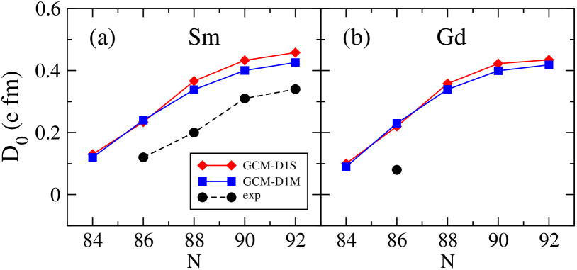
Figure 7: (Color online) The dynamical dipole moments provided by the GCM calculations for the nuclei ^146-154Sm and ^148-156Gd are shown, as functions of the neutron number, in panels a-b). Experimental dipole moments are taken from Ref. butler_96 . Results are shown for both Gogny-D1S and Gogny-D1M EDFs.

There are two spatial symmetries broken in the present calculations. One is rotational symmetry with the quadrupole moment as relevant parameter and the other is reflection symmetry (parity) with the octupole moment as relevant quantity. From the discussion of the mean field results it is clear that the softest mode is the octupole moment and therefore the most relevant symmetry to be restored is parity. Obviously, it would be desirable to restore also the rotational symmetry as well as particle number. This combined symmetry restoration is feasible but, when combined with the configuration mixing of next section, becomes a very demanding computational task not considered in this paper.

The quantum interference typical of the GCM framework could be directly used to restore the parity symmetry by choosing appropriate weights for the configurations with mutipole moments $(Q_{20},Q_{30})$ and $(Q_{20},-Q_{30})$ egi92 . However, in order to disentangle the relative contribution of the parity restoration correlations as compared with the ones of the GCM configuration mixing, we have carried out explicit parity projection calculations.

To restore parity symmetry mar83 ; egi91 we build positive ($\pi=+1$) and negative ( $\pi=-1$) parity-projected states $|{\Phi}^{\pi}(Q_{20},Q_{30})\rangle=\hat{{\cal{P}}}^{\pi}|{\Phi}(Q_{20},Q_{30})\rangle$ by applying the parity projector $\hat{{\cal{P}}}^{\pi}$ to the intrinsic configuration. The parity projector is a linear combination of the identity and the parity operator $\hat{\Pi}$ given by

$$\hat{{\cal{P}}}^{\pi}=\frac{1}{2}\left(1+\pi\hat{\Pi}\right).$$ (4)

The projected energies, used to construct parity-projected potential energy surfaces (to be called PPPES in what follows), are labeled with the multipole moments ${\bf Q}=(Q_{20},Q_{30})$ of the intrinsic state and read rob07

$$E_{\pi}({\bf Q})=\frac{\langle{\Phi}({\bf Q})|\hat{H}[\rho(\vec{r})]|{\Phi}({\bf Q})\rangle}{\langle{\Phi}({\bf Q})|{\Phi}({\bf Q})\rangle+\pi\langle{\Phi}({\bf Q})|\hat{\Pi}|{\Phi}({\bf Q})\rangle}+\pi\frac{\langle{\Phi}({\bf Q})|\hat{H}[\theta(\vec{r})]\hat{\Pi}|{\Phi}({\bf Q})\rangle}{\langle{\Phi}({\bf Q})|{\Phi}({\bf Q})\rangle+\pi\langle{\Phi}({\bf Q})|\hat{\Pi}|{\Phi}({\bf Q})\rangle}$$ (5)

The parity projected mean value of proton and neutron number, $\frac{\langle{\Phi}({\bf Q})|\hat{Z}\hat{{\cal{P}}}^{\pi}|{\Phi}({\bf Q})\rangle}{\langle{\Phi}({\bf Q})|\hat{{\cal{P}}}^{\pi}|{\Phi}({\bf Q})\rangle}$ and $\frac{\langle{\Phi}({\bf Q})|\hat{N}\hat{{\cal{P}}}^{\pi}|{\Phi}({\bf Q})\rangle}{\langle{\Phi}({\bf Q})|\hat{{\cal{P}}}^{\pi}|{\Phi}({\bf Q})\rangle}$ usually differ from the nucleus’ proton $Z_{0}$ and neutron $N_{0}$ numbers. To correct the energy for this deviation we have replaced $\hat{H}$ by $\hat{H}-\lambda_{Z}\left(\hat{Z}-Z_{0}\right)-\lambda_{N}\left(\hat{N}-N_{0}\right)$, where $\lambda_{Z}$ and $\lambda_{N}$ are chemical potentials for protons and neutrons, respectively har82 ; bon90 ; egi91 .

Figure 8: Predicted energy splittings between the lowest lying $\pi$=+1 and $\pi$=-1 2D-GCM states in ^146-154Sm and ^148-156Gd are compared with the experimental $0^{+}-1^{-}$ and $0^{+}-3^{-}$ splittings exp_ensdf . Results are shown for the D1S parametrization of the Gogny force as D1M ones are rather similar.

In the case of the Gogny-EDF, as well as for Skyrme-like EDFs, the definite expression for the projected energy (5) depends, on the prescription used for the density dependent part of the functional. In this work, we resort to the so called mixed density prescription that amounts to consider the standard intrinsic density

$$\rho(\vec{r})=\frac{\langle{\Phi}({\bf Q})|\hat{\rho}({\vec{r})}|{\Phi}({\bf Q})\rangle}{\langle{\Phi}({\bf Q})|{\Phi}({\bf Q})\rangle},$$ (6)

and the density

$$\theta(\vec{r})=\frac{\langle{\Phi}({\bf Q})|\hat{\rho}({\vec{r})}\hat{\Pi}|{\Phi}({\bf Q})\rangle}{\langle{\Phi}({\bf Q})|\hat{\Pi}|{\Phi}({\bf Q})\rangle}$$ (7)

in the evaluation of the first and second terms in Eq. (5), respectively. The mixed density prescription has been widely and successfully used in the context of projection and/or configuration mixing techniques (see, for example, bon90 ; rod02 ; egi04 ; review-Bender ; delta2p-2 ; Duguet-1 ; Doba-mixed and references therein). In fact, this is the only prescription that guarantees various consistency requirements within the EDF framework rod02 ; rob07 ; Duguet-kernels-1 . Even though this prescription has some drawbacks, as put into evidence recently Duguet-kernels-1 ; Duguet-kernels-2 ; Duguet-kernels-3 , the use of other prescriptions, like the one based on the projected density, are pathologically ill defined when applied to the restoration of spatial symmetries rob10b .

As an illustrative example of PPPES, we show in Fig. 4 the results for the nucleus ¹⁵⁰Sm obtained with both the D1S and D1M parametrizations of the Gogny force. Along the $Q_{30}$=0 axis, the projection onto positive parity $\pi$=+1 is unnecessary since the corresponding (quadrupole deformed) intrinsic configurations are already parity eigenstates with eigenvalue $\pi=+1$. For the same reason, the negative parity $\pi=-1$ projected wave function only makes sense along the $Q_{30}$=0 axis when a limiting procedure is considered. The evaluation of physical quantities in this case is subject to numerical inaccuracies consequence of evaluating the ratio of two small quantities (the denominator is the norm of the projected negative parity state that is zero in this case) and alternative expressions, obtained by considering explicitly the $Q_{30}$= 0 limit egi91 , are required for a sound numerical evaluation of those quantities. Note however (see, Fig. 5) that the negative parity projected energy increases rapidly while approaching the $Q_{30}$=0 configuration and therefore it does not play a significant role in the subsequent discussion of the corresponding PPPESs. As a consequence, we have omitted this quantity along the $Q_{30}$=0 axis.

As in the mean field case, the results with D1S and D1M show a striking similarity and therefore only the D1S results will be discussed. The comparison between the MFPESs in Fig. 1 and the PPPESs in Fig. 4, clearly illustrates the topological changes induced by the restoration of the reflection symmetry. In general, the quadrupole moments $Q_{20}$ corresponding to the absolute minima of the PPPESs, remain quite close to the ones obtained at the HFB level (see, Tables I and II) increasing their values as more neutrons are added for each of the Sm and Gd chains. On the other hand, the situation is quite different along the $Q_{30}$ direction. To obtain a more quantitative understanding of the evolution of the PPPESs, we have plotted in Fig. 5 the parity-projected energy curves for selfconsistent $Q_{20}$ values, as a function of the octupole moment $Q_{30}$ for the nucleus ¹⁵⁰ Sm. The corresponding HFB energy curves are also included for comparison. For ¹⁵⁰Sm, and all the other nuclei considered in the present study, the negative parity curves always show a well developed minimum at $Q_{30}$ values in the range 1.50-1.75 b^3/2. On the other hand, and regardless of the particular version of the Gogny-EDF employed, the $\pi=+1$ curves always display a characteristic pocket butler_96 ; bon88 ; egi91 with a minimum at $Q_{30}$ = 0.50-0.75 b^3/2. In the spirit of the Variation after Projection procedure, the configuration yielding the minimum of the positive (negative) parity projected energy as a function of $Q_{20}$ and $Q_{30}$ is to be associated with the positive (negative) parity state. As a consequence of this ”minimization after projection” the intrinsic states for each parity have different deformations. The positive parity ground state gains an amount of energy $E_{corr}^{\textrm{par proj}}$ given by

$$E_{corr}^{\textrm{par proj}}=E_{HFB}^{g.s.}-E_{\pi=+1}^{g.s.}$$ (8)

where, $E_{\pi=+1}^{g.s.}$ corresponds to the absolute minima of the positive parity PPPESs and $E_{HFB}^{g.s.}$ to the HFB ground state energies, i.e., the absolute minima of the MFPESs. Regardless of the Gogny-EDF employed, they are always smaller than 900 keV in each of the considered nuclei. This correlation energy has to be compared to the correlation energy gained by configuration mixing (see also Fig. 10 below).

IV Generator Coordinate Method.

According to the discussions in previous sections, it can be concluded that not only the plain HFB results of Sec. II, but even the parity projection ones, may not be sufficient to decide whether, as suggested in Ref. zhang_10 , there exists a transition to an octupole deformed regime in the considered nuclei in addition to the transitional behavior along the $Q_{20}$-direction ours_x5_1 ; ours_x5_2 . Within this context, $(Q_{20},Q_{30})$-GCM calculations are needed in order to verify the stability of the quadrupole and/or octupole deformation effects encountered in both the MFPESs and the PPPESs for the considered Sm and Gd nuclei. One should also keep in mind that in the framework of such a dynamical 2D-GCM treatment, not only the mean field energy surface but also the underlying collective inertia plays a role.

Figure 9: Theoretical and experimental transition rates $B(E1,1^{-}\rightarrow 0^{+})$ (panels a and b) and $B(E3,3^{-}\rightarrow 0^{+})$ (panels c and d) for the nuclei ^146-154Sm and ^148-156Gd. Results are shown for the Gogny-EDFs D1S and D1M. Experimental results for $B(E1,1^{-}\rightarrow 0^{+})$ rates are extracted from Ref. butler_96 while the experimental $B(E3,3^{-}\rightarrow 0^{+})$ rates are taken from Ref. Kibedi .

The superposition of HFB states

$$|{\Psi}_{\sigma}^{\pi}\rangle=\int d{\bf Q}f_{\sigma}^{\pi}({\bf Q})|{\Phi}({\bf Q})\rangle$$ (9)

is used to define the GCM wave functions $|{\Psi}_{\sigma}^{\pi}\rangle$. In the integration domain both positive and negative octupole moments $Q_{30}$ are included. The GCM amplitudes $f_{\sigma}^{\pi}({\bf Q})$ are the solutions of the Hill-Wheeler (HW) equation rs

$$\int d{\bf Q}^{{}^{\prime}}\left({\cal{H}}({\bf Q},{\bf Q}^{{}^{\prime}})-E_{\sigma}^{\pi}{\cal{N}}({\bf Q},{\bf Q}^{{}^{\prime}})\right)f_{\sigma}^{\pi}({\bf Q}^{{}^{\prime}})=0.$$ (10)

The GCM hamiltonian ${\cal{H}}({\bf Q},{\bf Q}^{{}^{\prime}})$ and norm ${\cal{N}}({\bf Q},{\bf Q}^{{}^{\prime}})$ kernels are given by

$${\cal{H}}({\bf Q},{\bf Q}^{{}^{\prime}}) = \langle{\Phi}({\bf Q})|\hat{H}[\rho^{GCM}(\vec{r})]|{\Phi}({\bf Q}^{{}^{\prime}})\rangle,$$

$${\cal{N}}({\bf Q},{\bf Q}^{{}^{\prime}}) = \langle{\Phi}({\bf Q})|{\Phi}({\bf Q}^{{}^{\prime}})\rangle$$ (11)

where in the evaluation of ${\cal{H}}({\bf Q},{\bf Q}^{{}^{\prime}})$ the mixed density prescription is used

$$\rho^{GCM}(\vec{r})=\frac{\langle{\Phi}({\bf Q})|\hat{\rho}({\vec{r})}|{\Phi}({\bf Q}^{{}^{\prime}})\rangle}{\langle{\Phi}({\bf Q})|{\Phi}({\bf Q}^{{}^{\prime}})\rangle}.$$ (12)

As in the parity projection case the Hamiltonian kernel ${\cal{H}}({\bf Q},{\bf Q}^{{}^{\prime}})$ is also supplemented with first order corrections in both proton and neutron numbers har82 ; bon90 ; egi91 .

The solution of the HW equation (10) provides the energies $E_{\sigma}^{\pi}$ corresponding to the ground ($\sigma=1$) and excited ($\sigma=2,3,\dots$) states. The parity of each of these states is given by the behavior of $f_{\sigma}^{\pi}({\bf Q})$ under the $Q_{30}\rightarrow-Q_{30}$ exchange. This is a consequence of the invariance under reflection symmetry of the GCM Hamiltonian kernels. For details on the solution of Eq. (10), the reader is referred, for example, to Refs. rs ; rod02 ; bon90 . Since the $|{\Phi}({\bf Q})\rangle$ basis states are not orthogonal, the functions $f_{\sigma}^{\pi}({\bf Q})$ of Eq. (9) can not be interpreted as probability amplitudes. One then introduces (see, for example, Refs. rs ; rod02 ) the collective wave functions

$$G_{\sigma}^{\pi}({\bf Q})=\int d{\bf Q}^{{}^{\prime}}{\cal{N}}^{\frac{1}{2}}({\bf Q},{\bf Q}^{{}^{\prime}})f_{\sigma}^{\pi}({\bf Q}^{{}^{\prime}}),$$ (13)

which are orthogonal and therefore their modulus squared $|G_{\sigma}^{\pi}({\bf Q})|^{2}$ has the meaning of a probability amplitude. It is easy to show that the parity of the collective wave functions $G_{\sigma}(Q_{20},Q_{30})$ under the exchange $Q_{30}\rightarrow-Q_{30}$ corresponds to the spatial parity operation in the correlated wave functions built up from them. The inclusion of octupole correlations immediately restores the reflection symmetry spontaneously broken at the mean field level and grants the use of a parity label $\pi$ for the GCM quantities.

The collective wave functions of Eq. (13) can be used to express overlaps of operators between GCM wave functions in a more convenient way

$$\langle\Psi_{\sigma}^{\pi}|\hat{O}|\Psi_{\sigma^{\prime}}^{\pi^{\prime}}\rangle=\int d{\bf Q}d{\bf Q}^{{}^{\prime}}G_{\sigma}^{\pi\,*}({\bf Q}){\cal O}({\bf Q},{\bf Q}^{{}^{\prime}})G_{\sigma^{\prime}}^{\pi^{\prime}}({\bf Q}^{{}^{\prime}}),$$ (14)

with the kernels

$${\cal{O}}({\bf Q},{\bf Q}^{{}^{\prime}})=\int d{\bf Q}^{{}^{\prime\prime}}d{\bf Q}^{{}^{\prime\prime\prime}}{\cal{N}}^{-\frac{1}{2}}({\bf Q};{\bf Q}^{{}^{\prime\prime}})\langle{\bf Q}^{{}^{\prime\prime}}|\hat{O}|{\bf Q}^{{}^{\prime\prime\prime}}\rangle{\cal{N}}^{-\frac{1}{2}}({\bf Q}^{{}^{\prime\prime\prime}};{\bf Q}^{{}^{\prime}})$$ (15)

given in terms of the operational square root of the overlap kernel that is defined by the property

$${\cal{N}}({\bf Q};{\bf Q}^{{}^{\prime}})=\int d{\bf Q}^{{}^{\prime\prime}}{\cal{N}}^{\frac{1}{2}}({\bf Q};{\bf Q}^{{}^{\prime\prime}}){\cal{N}}^{\frac{1}{2}}({\bf Q}^{{}^{\prime\prime}};{\bf Q}^{{}^{\prime}}).$$ (16)

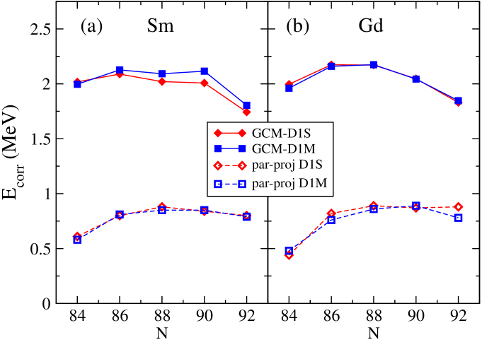
Figure 10: (Color online) The 2D-GCM correlation energies for the nuclei ^146-154Sm (panel a) and ^148-156Gd (panel b) are shown, as functions of the neutron number. The correlation energies stemming from the restoration of reflection symmetry are also included. Results are shown for both Gogny-D1S and Gogny-D1M EDFs. For more details, see main text.

The solution of Eq. (10) allows the calculation of physical observables like the energy splitting between positive and negative parity states as well as B(E1) and B(E3) transition probabilities. In the present study time reversal symmetry is preserved and therefore only excited states with an average angular momentum zero can be accounted for. Genuine $1^{-}$ and $3^{-}$ states, on the other hand, will require to consider cranking HFB states rs ; gar98 , a calculation which is out of the scope of the present work. We assume here that the cranking rotational energy of the $1^{-}$ and $3^{-}$ states is much smaller than the excitation energy of the negative-parity bandhead and therefore it can be neglected. For the reduced transition probabilities $B(E1,1^{-}\rightarrow 0^{+})$ and $B(E3,3^{-}\rightarrow 0^{+})$ the rotational model approximation for K=0 bands has been used

$$B(E\lambda,\lambda^{-}\rightarrow 0^{+})=\frac{e^{2}}{4\pi}\Big{|}\langle\Psi_{\sigma}^{\pi=-1}|\hat{{\cal O}}_{\lambda}|\Psi_{\sigma=1}^{\pi=+1}\rangle\Big{|}^{2}$$ (17)

where $\sigma$ corresponds to the first GCM excited state of negative parity. The electromagnetic transition operators $\hat{\cal{O}}_{1}$ and $\hat{\cal{O}}_{3}$ represent the dipole moment operator of Eq. (3) and the proton component $\hat{Q}_{30,\textrm{prot}}$ of the octupole operator, respectively. The evaluation of the overlap is carried out using Eq. (14).

In Fig. 6 the collective probability amplitude $|G_{\sigma}^{\pi}(Q_{20},Q_{30})|^{2}$ of Eq. (13), obtained from the solution of the HW equation (10) are plotted. As a typical example, results for the ^146,150,154Sm isotopes and the Gogny-D1S EDF are presented. For other nuclei and Gogny parametrizations, the results look very similar. The left panels in Fig. 6 correspond to the ground state wave functions (i.e., $\sigma=1$ and $\pi$=+1) while the right panels correspond to the lowest-lying $\pi$=-1 states $\sigma=3$ for ¹⁴⁶Sm and $\sigma=2$ for the others.

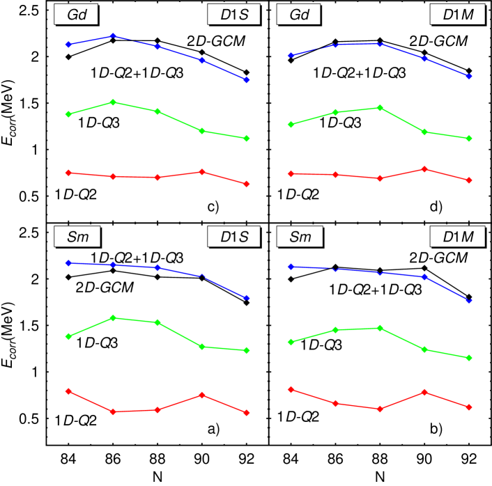
Figure 11: (Color online) The sum (blue curve named 1D-Q2+1D-Q3) of the correlation energies $E_{corr}^{1D-Q3}$ [Eq.(22)] (green curve named 1D-Q3) and $E_{corr}^{1D-Q2}$ [Eq.(24)] (red curve named 1D-Q2) is compared with the correlation energy $E_{corr}^{2D-GCM}$ [Eq.(20)] (black curve named 2D-GCM) provided by the full 2D-GCM calculations in ^146-154Sm and ^148-156Gd. Results are shown for both Gogny-D1S and Gogny-D1M EDFs. For more details, see main text.

The ground state collective probability amplitude $|G_{\sigma=1}^{\pi=+1}(Q_{20},Q_{30})|^{2}$ reach a global maximum at $Q_{30}=0$ pointing to the octupole-soft character of the ground states in ^146-154Sm. The spreading along the octupole direction is large for ^150,154Sm indicating octupole softness in these nuclei. For the negative parity collective wave functions the maximum is always located at a non zero value of $Q_{30}$ as could be anticipated from the parity projection results. For ^150,154Sm the wave function spreads out farther along $Q_{30}$ than in previous cases in agreement with the octupole softness of their ground states.

To have a more quantitative characterization of the collective wave functions we have computed mean values of relevant operators (see Eq. (14)). The first is the average of the quadrupole moment defined as

$$(\bar{Q}_{20})_{\sigma}^{\pi}=\langle{\Psi}_{\sigma}^{\pi}|\hat{Q}_{20}|{\Psi}_{\sigma}^{\pi}\rangle.$$ (18)

For negative parity operators like the octupole or the dipole moment the above averages are zero by construction and therefore a meaningful averaged quantity has to be defined as

$$\bar{O}_{\sigma}^{\pi}=4\int_{Q_{30}>0,Q_{30}^{{}^{\prime}}>0}d{\bf Q}d{\bf Q^{\prime}}G_{\sigma}^{\pi\,*}({\bf Q}){\cal O}({\bf Q},{\bf Q}^{{}^{\prime}})G_{\sigma}^{\pi}({\bf Q}^{{}^{\prime}})$$ (19)

where a restriction to positive values of the octupole moment has been made. The average quadrupole $\bar{Q}_{20}^{(+)}$ and octupole $\bar{Q}_{30}^{(+)}$ moments for the ground state ($\sigma=1$) are listed in Tables III and IV. The $\bar{Q}_{20}^{(+)}$ moments follow a trend similar to the one found within the HFB approximation increasing their values as more neutrons are added in a given isotopic chain. On the other hand, the isotopic trend predicted for $\bar{Q}_{30}^{(+)}$ is quite different to the one predicted at the mean field level. As discussed in Sec. II, at the Gogny-HFB level only the N=86 and 88 isotones ^148,150Sm and ^150,152Gd display non vanishing (static) octupole moments (see, Tables I and II). Nevertheless, after both projection onto $\pi=+1$ and dynamical $(Q_{20},Q_{30})$-fluctuations are considered at the 2D-GCM level, the octupole deformation effects predicted for ^148,150Sm and ^150,152Gd are reduced to more than half of their mean field values. At variance with the HFB results, the nuclei ^146,152,154Sm and ^148,154,156Gd exhibit dynamical ground state octupole moments $\bar{Q}_{30}^{(+)}\approx$ 0.40-0.50 b^3/2. We conclude that, regardless of the particular version of the Gogny-EDF employed, our 2D-GCM calculations suggest a dynamical shape/phase transition from weakly (¹⁴⁶Sm and ¹⁴⁸Gd) to well quadrupole deformed (¹⁵⁴Sm and ¹⁵⁶Gd) ground states as well as a transition to an octupole vibrational regime in the considered Sm and Gd nuclei.

For the lowest-lying negative parity states, the dynamical octupole $\bar{Q}_{30}^{(-)}$ and quadrupole $\bar{Q}_{20}^{(-)}$ moments, computed with the corresponding 2D-GCM states $|{\Psi}_{\sigma=2}^{\pi=-1}\rangle$ or $|{\Psi}_{\sigma=3}^{\pi=-1}\rangle$, are also listed in Tables III and IV. It should be noted that the largest values of the octupole deformations $\bar{Q}_{30}^{(+)}$ and $\bar{Q}_{30}^{(-)}$ always correspond to the N=88 isotones ¹⁵⁰Sm and ¹⁵²Gd.

The values of the ground state dipole moments $\bar{D}_{0}^{(+)}$ are less predictable than the averages of the quadrupole and octupole moments discussed previously as the behavior of $D_{0}$ for the HFB states strongly depends upon the orbitals occupied and those change rapidly with deformation. The comparison of the dipole moments with available experimental data butler_96 is presented in panels a) and b) of Fig. 7. In particular, the comparison between the HFB results (see, Tables I and II), $\bar{D}_{0}^{(+)}$ and experimental values clearly reveal the limitations of the HFB approximation to predict dipole moments in this region of the nuclear chart.

Another physical observable is the energy splitting between the lowest lying $\pi=+1$ and $\pi=-1$ states. The results for ^146-154 Sm and ^148-156Gd are compared in Fig. 8 with available experimental $0^{+}-1^{-}$ and $0^{+}-3^{-}$ energy splittings exp_ensdf . As already mentioned, in the present study we are not able to account for genuine $1^{-}$ and/or $3^{-}$ states that require, for example, the use of cranking HFB states rs ; gar98 . With this in mind and regardless of the Gogny-EDF employed, a reasonable agreement between the theoretical and experimental energy splittings is observed. The remaining discrepancies imply that correlations other than (axial) quadrupole-octupole fluctuations could also be required. In particular, the time-odd components of the Gogny-EDF, incorporated throughout cranking calculations, should be further investigated within the present 2D-GCM framework. Let us mention that the results are compatible with the ones obtained in Ref. egi92 using a one-dimensional collective Hamiltonian whose parameters are derived from octupole constrained calculations. This is also the case with the systematic calculations of Ref. rob11b using a GCM with the octupole degree of freedom as generating coordinate.

In panels a) and b) of Fig. 9, the $B(E1,1^{-}\rightarrow 0^{+})$ reduced transition probabilities of Eq. (17) are compared with experimental data butler_96 . It is very satisfying to observe how, without resorting to any effective charges, the predicted $B(E1,1^{-}\rightarrow 0^{+})$ values in Sm nuclei follow the experimental isotopic trend with a slight improvement in the case of the Gogny-D1M EDF. In panels c) and d) of the same figure, we compare the $B(E3,3^{-}\rightarrow 0^{+})$ transition rates of Eq. (17)] with available data Kibedi . The predicted $B(E3,3^{-}\rightarrow 0^{+})$ values reproduce quite well the experimental ones in the case of ^152,154Sm and ^154,156Gd. On the other hand, from the comparison between ours and the $B(E1,1^{-}\rightarrow 0^{+})$ and $B(E3,3^{-}\rightarrow 0^{+})$ rates obtained in Refs. egi92 and rob11b , we can conclude that they are, to a large extent, not very sensitive to quadrupole fluctuations.

In panels a) and b) of Fig. 10, the correlation energies defined as the difference between the reference HFB ground state energy and the 2D-GCM one

$$E_{corr}^{2D-GCM}=E_{HFB}^{g.s}-E_{\sigma=1}^{\pi=+1}$$ (20)

are ploted. The parity restoration correlation energies $E_{corr}^{\textrm{par proj}}$ of Eq. (8) are also included for comparison. The predicted isotopic trends and quantitative values of $E_{corr}^{2D-GCM}$ are quite similar for both Gogny-D1S and Gogny-D1M EDFs. The correlation energies $E_{corr}^{2D-GCM}$ exhibit a relatively weak dependence with neutron number with values oscillating between 1.74 and 2.09 MeV for Sm and between 1.83 and 2.17 MeV for Gd nuclei. The smooth variation of the correlation energy is, however, of the same order of magnitude as the rms for the binding energy in modern nuclear mass tables gogny-d1m and therefore the dynamical octupole correlation energies should be considered in improved versions of them.

A rough estimate of the contribution of the $(Q_{20},Q_{30})$ fluctuations to the correlation energies can be obtained by subtracting to the total correlation energy the parity projected one. Those contributions range in between 0.94 and 1.41 MeV for Sm isotopes and in between 0.94 and 1.56 MeV for Gd isotopes. The oscillations are slightly larger than for the total correlation energy.

In order to determine the contributions of each degree of freedom in the results obtained we have also performed one dimensional GCM calculations along each of the degrees of freedom. First, the octupole moment has been used as generating coordinate. For each octupole moment considered the quadrupole moment corresponds to the minimum energy. The octupole moments of the generating wave functions are taken in the range -7 b^3/2 $\leq Q_{30}\leq$ 7 b^3/2 and with a mesh size $\delta Q_{30}$= 0.25 b^3/2. The 1D-GCM ansatz is

$$|{\Psi}_{\sigma,1D-Q3}^{\pi}\rangle=\int dQ_{30}f_{\sigma,1D-Q3}^{\pi}(Q_{30})|{\Phi}(Q_{30})\rangle$$ (21)

given in terms of the HFB states $|{\Phi}(Q_{30})\rangle$. Note that no quadrupole constraint is imposed in these calculations. From the 1D-Q3 ground state energies we can computed the 1D octupole correlation energy

$$E_{corr}^{1D-Q3}=E_{HFB}^{g.s}-E_{\sigma=1,1D-Q3}^{\pi=+1}$$ (22)

This quantity is displayed in panels a) to d) of Fig. 11 for the considered Sm and Gd nuclei. It has to be mentioned that this type of calculations have been carried out for all possible even-even nuclei with several parametrizations of the Gogny force in rob11b .

In a second step, GCM calculations with the quadrupole degree of freedom ($Q_{30}=0$, i.e., reflection symmetry is preserved) as generating coordinate have been performed. The $Q_{20}$ values used are in the interval -30b $\leq Q_{20}\leq$ 30b with $\delta Q_{20}$= 0.6 b. The GCM wave functions

$$|{\Psi}_{\sigma,1D-Q2}\rangle=\int dQ_{20}f_{\sigma,1D-Q2}(Q_{20})|{\Phi}(Q_{20})\rangle$$ (23)

are defined in terms of the states $|{\Phi}(Q_{20})\rangle$. The corresponding correlation energy

$$E_{corr}^{1D-Q2}=E_{HFB}^{g.s}-E_{\sigma=1,1D-Q2}$$ (24)

is displayed in panels a) to d) of Fig. 11.

In panels a) to d) of Fig. 11, we compare the sum $E_{corr}^{1D-Q2+1D-Q3}=E_{corr}^{1D-Q3}+E_{corr}^{1D-Q2}$ with the correlation energies $E_{corr}^{2D-GCM}$ of Eq. (20). For the particular set of Sm and Gd nuclei considered in the present study and regardless of the Gogny-EDF employed, the correlation energies provided by the full 2D-GCM are very well reproduced by the sum of the ones obtained in the framework of the 1D-GCM approximations (21) and (23). Obviously, this is far from being a general statement and further explorations in other regions of the nuclear chart, specially those showing shape coexistence already at $Q_{30}=0$ are required. Nevertheless, the kind of decoupling observed in our results may be potentially relevant to incorporate correlation energies stemming from parity restoration and octupole fluctuations in large scale calculations of nuclear masses based on the Gogny-EDF (see, for example, delaroche10 ) as well as in future fitting protocols beyond the most recent D1M parametrization gogny-d1m of the Gogny EDF.

V Conclusions

Calculations have been carried out using the GCM method and with the multipole moments $Q_{20}$ and $Q_{30}$ as generating coordinates for several Sm and Gd isotopes and with different parametrizations of the Gogny force. The results from different parametrizations are very close to each other indicating again that the D1M parametrization of the Gogny force performs as well as D1S in spectroscopic calculation. The comparison with experimental data is fairly good both for excitation energies and electromagnetic transition probabilities reassuring the predictive power of the Gogny class of EDFs. Comparison of the 2D GCM results with the outcome of previous 1D Collective Schrodinger equation calculations in the same region points out to a decoupling of the dynamics of the quadrupole and octupole degrees of freedom. This conclusion is reinforced by the comparison of the 2D correlation energies with the sum of correlation energies along each of the degrees of freedom. Correlation energies show a smooth behavior with neutron number with differences between different isotopes as large as 200 keV. Although these differences are small, they can be relevant for theories aiming at providing accurate mass tables for applications requiring accurate reaction rates that depend on their energetic balance.

- (1) P.A. Butler and W. Nazarewicz, Rev. Mod. Phys. 68, 349 (1996).
- (2) R.F. Casten and N.V. Zamfir, Phys. Rev. Lett. 87, 052503 (2001); R. Krücken et al., Phys. Rev. Lett. 88, 232501 (2002).
- (3) F. Iachello, Phys. Rev. Lett. 87, 052502 (2001).
- (4) J. Meng, W. Zhang, S.G. Zhou, H. Toki, and L.S. Geng, Eur. Phys. J. A 25, 23 (2005); Z.P. Li, T. Niksic, D. Vretenar, J. Meng, G.A. Lalazissis, and P. Ring, Phys. Rev. C 79, 054301 (2009).
- (5) R. Rodríguez-Guzmán and P. Sarriguren, Phys. Rev. C76, 064303 (2007).
- (6) L.M. Robledo, R.R. Rodríguez-Guzmán, and P. Sarriguren, Phys. Rev. C78, 034314 (2008).
- (7) T. R. Rodríguez and J.L.Egido, Phys. Lett. B663, 49 (2008).
- (8) S. Aberg, H. Flocard, and W. Nazarewicz, Ann. Rev. Nucl. Part. Sci. 40, 439 (1990).
- (9) W. Urban et al., Phys. Lett. B185, 331 (1987).
- (10) W. Urban et al., Phys. Lett. B258, 293 (1991).
- (11) P.E. Garrett et al., Phys. Rev. Lett. 103, 062501 (2009).
- (12) D. Vretenar, A. V. Afanasjev, G. A. Lalazissis and P. Ring, Phys. Rep. 409, 101 (2005).
- (13) M. Bender, P.-H. Heenen and P.-G.Reinhard, Rev. Mod. Phys. 75, 121 (2003).
- (14) J. Dechargé and D. Gogny, Phys. Rev. C 21, 1568 (1980).
- (15) J. F. Berger, M. Girod, and D. Gogny, Nucl. Phys. A428, 23c (1984).
- (16) M. Baldo, P. Schuck, and X. Viñas, Phys. Lett. B663, 390 (2008).
- (17) P. Möller and J.R. Nix, Nucl. Phys. A361, 117 (1981).
- (18) G.A. Leander, R.K. Sheline, P. Möller, P. Olanders, I. Ragnarsson, and A.J. Sierk, Nucl. Phys. A388, 452 (1982).
- (19) W. Nazarewicz et al., Nucl. Phys. A429, 269 (1984).
- (20) W. Nazarewicz and S.L. Tabor, Phys. Rev. C 45, 2226 (1992).
- (21) S. Marcos, H. Flocard, and P.H. Heenen, Nucl. Phys. A410, 125 (1983).
- (22) P. Bonche, P. -H. Heenen, H. Flocard, and D. Vautherin, Phys. Lett. B175, 387 (1986).
- (23) P.Bonche, The Variety of Nuclear Shapes, edited by J.D.Garret et al., World Scientific, Singapore, page 302 (1988).
- (24) P. Bonche, J.S. Krieger, M.S. Weiss, J. Dobaczewski, H. Flocard, and P.-H. Heenen, Phys. Rev. Lett. 66, 876 (1991).
- (25) P.-H. Heenen, J. Skalski, P.Bonche, and H. Flocard, Phys. Rev. C 50,802 (1994).
- (26) J. Meyer, P. Bonche, M.S. Weiss, J. Dobaczewski, H. Flocard, and P.-H. Heenen, Nucl. Phys. A588, 597 (1995).
- (27) L.M. Robledo, J.L. Egido, J.F. Berger, and M. Girod, Phys. Lett. B187, 223 (1987).
- (28) L.M. Robledo, J.L. Egido, B. Nerlo-Pomorska, and K. Pomorski, Phys. Lett. B201, 409 (1988).
- (29) J.L. Egido and L.M. Robledo, Nucl. Phys. A518, 475 (1990).
- (30) J.L. Egido and L.M. Robledo, Nucl. Phys. A524, 65 (1991).
- (31) E. Garrote, J.L. Egido, and L.M. Robledo, Phys. Rev. Lett. 80, 4398 (1998); Nucl. Phys. A654, 723c (1999).
- (32) L.M. Robledo, M. Baldo, P. Schuck, and X. Viñas, Phys. Rev. C 81,034315 (2010).
- (33) J.L. Egido and L.M. Robledo, Nucl. Phys. A545, 589 (1992).
- (34) M. Babilon, N.V. Zamfir, D. Kusnezov, E.A. McCutchan, and A. Zilges, Phys. Rev. C 72, 064302 (2005).
- (35) N. Minkov, P. Yotov, S. Drenska, W. Scheid, D. Bonatsos, D. Lenis, and D. Petrellis, Phys. Rev. C 73, 044315 (2006).
- (36) P.G. Bizzeti and A.M. Bizzeti-Sona, Phys. Rev. C 81, 034320 (2010).
- (37) J. Skalski, Phys. Rev. C 43, 140 (1991).
- (38) W. Zhang, Z.P. Li, S.Q. Zhang, and J. Meng, Phys. Rev. C 81, 034302 (2010).
- (39) W. H. Long, J. Meng, N. Van Giai, and S. G. Zhou, Phys. Rev. C 69, 034319 (2004).
- (40) R. Rodríguez-Guzmán, P. Sarriguren, L.M. Robledo and J.E. García-Ramos, Phys. Rev. C 81, 024310 (2010).
- (41) P. Ring and P. Schuck, The Nuclear Many-Body Problem (Springer, Berlin-Heidelberg-New York) (1980).
- (42) P.-H. Heenen, A. Valor, M. Bender, P. Bonche, and H. Flocard, Eur. Phys. J. A 11, 393 (2001)
- (43) S. Goriely, S. Hilaire, M. Girod, and S. Péru, Phys. Rev. Lett. 102, 242501 (2009).
- (44) R. R. Rodríguez-Guzmán, J. L. Egido, and L.M. Robledo, Nucl. Phys. A709, 201 (2002).
- (45) J.L Egido and L.M. Robledo, Lecture Notes in Physics 641, 269 (2004).
- (46) J.L. Egido, L.M. Robledo and R.R. Rodríguez-Guzmán, Phys. Rev. Lett. 93 , 082502 (2004).
- (47) J. F. Berger, M. Girod and D. Gogny, Nucl. Phys. A502, 85c (1989).
- (48) C. R. Chinn, J. F. Berger, D. Gogny, and M. S. Weiss, Phys. Rev. C 45, 1700 (1992).
- (49) M. Girod, J.P. Delaroche, D. Gogny and J.F. Berger, Phys. Rev. Lett. 62, 2452 (1989).
- (50) G. F. Bertsch, M. Girod, S. Hilaire, J.-P. Delaroche, H. Goutte, and S. Péru, Phys. Rev. Lett. 99, 032502 (2007).
- (51) S. Péru, J. F. Berger, and P. F. Bortignon, Eur. Phys. J. A 26, 25 (2005).
- (52) S. Hilaire and M. Girod, Eur. Phys. J. A 33, 33 (2007).
- (53) J.-P. Delaroche, M. Girod, J. Libert, H. Goutte, S. Hilaire, S. Péru, N. Pillet and G.F. Bertsch, Phys. Rev. C 81, 014303 (2010).
- (54) R. Rodríguez-Guzmán, P. Sarriguren, L.M.Robledo and S.Perez-Martin, Phys. Lett. B691, 202 (2010).
- (55) L.M. Robledo, R. Rodríguez-Guzmán and P. Sarriguren, J. Phys. G: Nucl. Part. Phys. 36, 115104 (2009).
- (56) R. Rodríguez-Guzmán, P. Sarriguren and L.M.Robledo, Phys. Rev. C 82, 044318 (2010).
- (57) R. Rodríguez-Guzmán, P. Sarriguren and L.M.Robledo, Phys. Rev. C 82, 061302 (R) (2010).
- (58) R. Rodríguez-Guzmán, P. Sarriguren and L.M.Robledo, Phys. Rev. C 83, 044307 (2011).
- (59) L.M. Robledo and G.F. Bertsch, Phys. Rev C 84, 014312 (2011).
- (60) L.M. Robledo and G.F. Bertsch, Phys. Rev C 84, 054302 (2011).
- (61) A. Bohr and B.R. Mottelson, Nuclear Structure (Benjamin, New York, 1969 and 1975).
- (62) P. -G. Reinhard and E.W. Otten, Nucl. Phys. A420, 173 (1984).
- (63) L.M. Robledo, Int. J. Mod. Phys. E16, 337 (2007).
- (64) K. Hara, A. Hayashi and P.Ring, Nucl. Phys. A385, 14 (1982).
- (65) P. Bonche, J. Dobaczewski, H. Flocard, P.-H. Heenen and J. Meyer, Nucl. Phys. A510, 466 (1990).
- (66) M. Bender, G.F. Bertsch and P.-H. Heenen, Phys. Rev. Lett. 94, 102503 (2005).
- (67) T. Duguet, M. Bender, P. Bonche and P.-H. Heenen, Phys. Lett. B559, 201 (2003).
- (68) J. Dobaczewski, W. Satula, B.G. Carlsson, J. Engel, P. Olbratowski, P. Powalowski, M. Sadziak, J. Sarich, N. Schunck, A. Staszczak, M. Stoitsov, M. Zalewski and H. Zdunczuk, Comput. Phys. Commun. 180, 2361 (2009).
- (69) D. Lacroix, T. Duguet and M. Bender, Phys. Rev. C79, 044318 (2009).
- (70) M. Bender, T. Duguet and D. Lacroix, Phys. Rev. C79, 044319 (2009).
- (71) T. Duguet, M. Bender, K. Bennaceur, D. Lacroix and T. Lesinski, Phys. Rev. C79, 044320 (2009).
- (72) L.M. Robledo, J. Phys. G: Nucl. Part. Phys. 37, 064020 (2010).
- (73) T. Kibédi and ’R.H. Spear, At. Data Nucl. Data Tables 80, 35 (2002).
- (74) Evaluated Nuclear Structure Data Files (ENSDF): www.nndc.bnl.gov/ensdf.