The nuclear electric polarizability of 6He
Abstract
We present an estimate of the nuclear electric polarizability of the 6He halo nucleus based on six-body microscopic calculations. Wave functions are obtained from semi-realistic two-body interactions using the hyperspherical harmonics expansion method. The polarizability is calculated as a sum rule of the dipole response function using the Lanczos algorithm and also by integrating the photo-absorption cross section calculated via the Lorentz integral transform method. We obtain fm3, which is much smaller than the published value fm3 Moro extracted from experimental data. This points towards a potential disagreement between microscopic theories and experimental observations.
pacs:
21.10.Gv, 24.70.+s, 21.60.De, 27.20.+nI Introduction
The nuclear electric polarizability is related to the response of a nucleus to an externally applied electric field. It is an interesting observable because it encapsulates information about the excitation spectrum of a nucleus. Recently, it has attracted a lot of attention both for light nuclei, see e.g. Moro , and for heavy nuclei, see e.g. Pb_RCNP . For light systems the nuclear polarizability is relevant in the extraction of nuclear quantities from atomic spectroscopic measurements. The atomic energy levels are affected by polarization of the nucleus due to the electric field of the surrounding electrons. Such nuclear structure correction, which is proportional to noert where is the Bohr radius, needs to be considered in the sophisticated quantum electrodynamics calculations of the atomic levels that allow the extraction of charge radii from isotope shifts measurements of unstable nuclei, see Refs. Wan04 ; Maxime and Mue07 for 6He and 8He, respectively. An even larger effect of the nuclear structure correction coming from the polarizability is expected in muonic atoms, as the muon mass is larger than the electron mass and the orbital radius is smaller. This will be relevant to the proposed He and He experiments rolf_exp that aim at measuring the nuclear charge radius of 4He and 3He from the Lamb-shift, to be compared to electron scattering data.
The nuclear electric polarizability of Helium isotopes is interesting for the several above mentioned reasons. It has been already directly measured or extracted from experimental data for the 3,4,6He isotopes Moro . In the case of 3He it is worth mentioning that the data from elastic scattering on Pb at energies below the Coulomb barrier Goe91 are in disagreement with estimates based on calculations of the photo-absorption cross section Moro , the latter being about a factor of 2 smaller. It is also worth noticing that the theoretical calculations are in agreement with photo-absorption experiments, and that the band spanned by using different Hamiltonians in the calculations is smaller than the difference between the data taken from photo-absorption cross section and from ion scattering experiments. The data analysis involved in the latter approach is quite delicate, because one has to separate effects of the nuclear force from Coulomb effects.
In Ref. Stetcu the polarizabilities of several Hydrogen and Helium isotopes were calculated with ab-initio methods. Among the Helium isotopes, 3He and 4He were dealt with, but no prediction for 6He was provided. It is the aim of this paper to fill this gap.
The 6He is known as a halo nucleus, where a tightly bound 4He core is surrounded by two neutrons Tan96 . It happens to be the lightest of the known halo nuclei and it is a Borromean nucleus, because the two-neutron and neutron-core subsystems are unbound, but the three-body system is held together. Due to the very small separation energy which characterizes halo nuclei, one expects the polarizability of 6He to be much larger than that of the tightly bound 4He isotope. Experimental data indicate this behavior. In this paper we would like to see whether microscopic calculations reproduce the experimental values and lead to a result where ).
We perform a microscopic study of the nuclear polarizability for 6He and compare it to 4He. We limit our study to simple semi-realistic two-body forces. For that we use the hyperspherical harmonics method with an effective interaction, EIHH, to speed up the convergence Nir ; EIHH . The polarizability is calculated as a sum rule of the dipole response function using the Lanczos algorithm and also integrating the photo-absorption cross section calculated with the Lorentz integral transform method ELO94 .
This paper is organized as follows. In Section II we describe in details the theoretical calculation of the polarizability. In Section III we present our results and in Section IV we make a comparison with experiment. Finally, we conclude in Section V.
II Theoretical aspects
The nuclear electric polarizability in the unretarded dipole approximation is defined by the expression
| (1) |
where is the fine structure constant, is the unretarded dipole operator and are the energies of the nuclear ground and excited states and , respectively. This observable is clearly related to the photo-absorption cross section and to the dipole response function. The photo-absorption cross section of a nucleus is given by
| (2) |
where is the response function. In the unretarded dipole approximation
| (3) |
where indicates an average on the initial angular momentum projections. The dipole operator is given by , where is the number of nucleons and and are the third component of the isospin operator and the coordinate of the th particle in the center of mass frame, respectively. One can recover the expression for in Eq. (1) by calculating sum rules of the photo-nuclear cross section. The various moments of are defined as
| (4) |
where is the photon energy and and indicate threshold energy and upper integration limit, respectively. Assuming that converges to zero and utilizing the closure of the eigenstates of the nuclear Hamiltonian , one can relate the polarizability to the sum rule,
| (5) |
The polarizability can be calculated with the Lanczos algorithm using a proper pivot. It is useful to rewrite Eq. (5) as
| (6) | |||||
with
| (7) |
Starting from the “pivot” of Eq. (7) where the ground state is obtained by solving the Schrödinger equation, can be expressed as a continued fraction containing the Lanczos coefficients Dagotto
| (8) |
where the form the Lanczos orthonormal basis . In fact one has
| (9) |
In this work we calculate the polarizability in two different ways. On the one hand we utilize Eq. (9). On the other hand we obtain by integrating our results for the total photo-absorption cross section calculated with the Lorentz integral transform (LIT) method ELO94 . In Ref. He6Sonia1 ; He6Sonia2 we have presented microscopic calculations of the 6He with semi-realistic potential models. Here we use lager model spaces which are nowadays available. The LIT, an integral transform with a Lorentzian kernel, is defined as
| (10) |
The LIT is also typically calculated using the Lanczos technique explained above, (see Mario ). In fact it can be re-expressed as
| (11) |
with . It is evident that the LIT in (11) is also a continued fraction as in Eq. (9), where is replaced by a complex . Once is calculated, one can invert the LIT inversion to get , and thus . The two methods have to agree within the numerical uncertainty. However, with the first method one avoids the complications introduced by the inversion procedure.
Given the Hamiltonian , the calculation of in both ways is based on the EIHH EIHH expansion of the wave function. This approach is translational invariant, being constructed with the Jacobi coordinates. We use different semi-realistic potential models for our calculations. Following Ref. He6Sonia1 , we will use the Minnesota (MN) potential Minnesota
| (12) | |||||
where are spin and space-exchange operators, are parameterized as linear combination of Gaussians of the two-body relative distance and is a parameter. This force reproduces the wave nucleon-nucleon phase shifts and correctly binds the deuteron. It renormalizes effects of the tensor force into its central component. A typical value for in the Minnesota potential is , as we used in He6Sonia1 . Here we will explore the variation of this parameter by choosing . The mixing parameter does not affect the dominant and waves in the NN interaction, but only affects the , channels, where the dominant components are the waves ( and ). For there are no waves, they contribute only for . Thus, changing mostly affects 6He, without substantially changing 4He. Because in He6Sonia1 ; He6Sonia2 we also used the Malfliet-Tjon (MTI-III) MTI-III , and the Argonne AV4’ AV4' potentials, we will present some results with these interactions as well. The Minnesota potential has been recently used in a microscopic cluster model calculation of 6He Brida and in the Gamow shell model approach Papadim for 6He and 8He.
III Results and Discussion
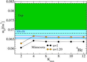
The main focus of this work is to study the 6He polarizability. We start, however, the discussion with the 4He nucleus. In Fig. 1, we show the results of calculated via the Lanczos coefficients, as in Eq. (9). The ground state and the Lanczos “pivot” are given in terms of the EIHH expansions. While for the ground state the expansion is characterized by an even hyperspherical grand-angular quantum number and total isospin , , has to be expanded on odd grand-angular quantum number , where the isospin in the final state is . Fig. 1 shows the convergence of as a function of , where for each point is used for the Lanczos “pivot”. We show our results for the Minnesota potential with 1 and 1.20. The convergence is very good, the dependence on is mild and the results are very close to calculations where realistic nucleon-nucleon (NN) and three-nucleon (3N) forces have been used. For the latter one, results for effective field theory potentials were presented in Stetcu leading to fm3 (corresponding to the upper light (blue) band in Fig. 1). The error bar of this calculation is accounting for the convergence error fm3 and also for the uncertainty in the underlying dynamics fm3. We also show the results of for the Argonne two-body force and Urbana IX three-body force of Ref. Gazit leading to (corresponding to the lower light (blue) band in Fig. 1), where the error bar comes from convergence only. The experimental data are shown as a darker (green) band. These include the more recent evaluation of Ref. Moro based on the Arkatov et al. Arkatov experimental measurement of the photo-absorption cross section and an older result reported in Ref. Friar , based on earlier measurements by Arkatov et al. Arkatov_old . We would like to point out that the semi-realistic Minnesota potentials lead to a value of the polarizability which is consistent with realistic calculations and is only about 15 smaller than the average value in the experimental band.
We can also calculate the polarizability by integrating the photoabsorption cross section obtained with the LIT method. We get perfect agreement as with the Lanczos coefficients. For example, for the standard Minnesota potential where and for a model space, the Lanczos method gives fm3 and integrating up to 120 MeV we get 0.06336 fm3, with just a difference.
Now we move to the 6He nucleus. We first calculate from the Lanczos coefficients. Also in this case the ground state is expanded on even hyperspherical grand-angular quantum number , but the total isospin is , , and is expanded on odd . In this case though, the final isospin can be or . This leads to two possible isospin channels that are calculated separately and that open up at different energies. Experimentally, the channel opens up at photon energy MeV, while the channel opens up at MeV, with He 3H. Due to the inverse energy weight in Eq. (5), the channel is expected to be less relevant to . From our calculations we find that the percentage contribution of the T=2 isospin channel to the total polarizability changes from to when varying from 1 to 1.20 in the Minnesota potential.
| Potential | (4He) | (6He) | (6He) |
|---|---|---|---|
| Minnesota | |||
| u=1.00 | -29.949 | -30.45 | 0.50 |
| u=1.05 | -29.978 | -31.13 | 1.15 |
| u=1.10 | -30.007 | -31.88 | 1.87 |
| u=1.15 | -30.037 | -32.72 | 2.68 |
| u=1.20 | -30.069 | -33.65 | 3.59 |
| MTI-III | -30.760 | -32.24 | 1.48 |
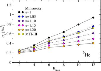
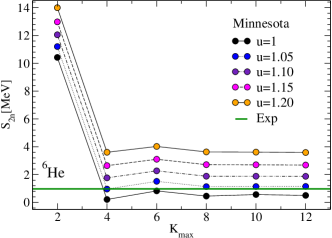
In Fig. 2, we present a similar plot as in Fig. 1 for 6He with semi-realistic interactions. We observe a much slower convergence of for 6He than for 4He with all the potentials employed. By looking at the different values in the Minnesota potential, we see that the convergence rate and the value of substantially change with . This is related to the variation of the binding energy, and consequently of the two-neutron separation energy, whose numerical values are shown in Table 1 for completeness. By increasing we are adding more wave interactions, which bring additional binding to the 6He nucleus, while leaving 4He almost unaffected. Naively, this makes 6He more tightly bound and thus more difficult to polarize, i.e., gets smaller. For the value of the convergence of the polarizability is particularly slow, due to the fact that 6He is barely bound, with MeV which is about a factor of 2 smaller than the experimental value. With the MTI-III potential we get a convergence pattern which is close to the Minnesota potential for , because the prediction of is similar with these two potentials, see Table 1. The information that one gains from Fig. 2 is that by increasing we can change the overall slope of the convergence pattern of .
For any considered value of though, it is clear that our calculations reproduce the fact that the polarizability of the halo nucleus of 6He is much larger than that of the tightly bound 4He, the ratio being almost an order of magnitude.
Here we would like to point out that Brida and Nunes in Brida have used the Minnesota potential with in a microscopic cluster model and obtained a separation energy MeV. This result is different from the value we obtain and report in Table 1. Their calculation is performed without the Coulomb force, but its effect cancels in the separation energy. Because for 4He the value reported in Brida for the binding energy is -30.85 MeV, which is in agreement with our value of -30.86(1) (with no Coulomb force), we think that the difference is due to the cluster assumption made for 6He. We do not make such assumption and in convergence, the EIHH result is exact. In Fig. 3, we show that the separation energy is very well converged within the model space available for all these potentials.
We can also calculate the polarizability by integrating the photoabsorption cross section obtained with the LIT method and compare it to the above results. We quote numbers for the Minnesota potential with in the largest available model space . The Lanczos method gives fm3 and integrating up to 40 MeV (60 MeV) we get 0.7711 fm3 (0.7827) fm3. Integrating the cross section we have a 3-4 difference, which is due to the fact that LIT is not completely converged and the inversion procedure introduces some numerical error.
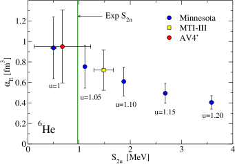
Now we would like to investigate the dependence of the polarizability on the two-neutron separation energy. This can be achieved for example by plotting versus for the different values of the parameter in the Minnesota potential. In Fig. 4, we can see that we find a correlation between and . Calculations have been performed with (). As an estimate of the theoretical error bar in the few-body method we take the difference between the largest possible calculation with and the result. We also present the data for the MTI-III and AV4’ potential (as used in He6Sonia2 ) for completeness. The error bars for the polarizability increase as the separation energy gets smaller. This is a reflection of the slower convergence observed in Fig. 2. For the Minnesota potential has a negligible error, hardly visible in Fig. 4. For the MTI-III and AV4’ potentials the error in is large because these interaction models are not as soft as the Minnesota force.
In Ref. Stetcu it was argued that the polarizability should roughly scale like the inverse square of the binding energy of a nucleus. For a halo system, like 6He, the relevant scale parameter is the separation energy, rather than the binding energy. The dependence empirically observed in Fig. 4 is compatible with such a behavior.
In order to reproduce the polarizability of a halo nucleus, it is expected that the halo structure, thus , should be correctly modeled, even if the absolute binding of 4He and 6He are not reproduced. Thus, one can estimate the value of by choosing to be around the experimental value and then calculate the corresponding polarizability. A value of that gives close to experiment is , where the convergence of is slower than for larger values of . From a closer look to Fig. 2 and Fig. 3 we can see that also for the polarizability is still increasing when becomes larger, even though the separation energy is converged. This means that the convergence of the polarizability is not only influenced by . Other observable that is naturally related to the polarizability in the unretarded dipole approximation is the radius operator.
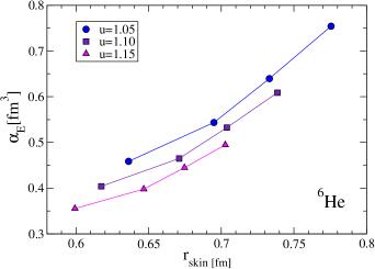
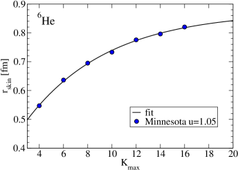
In recent papers Pb_theory ; Shlomo the correlation between the polarizability and the neutron skin of the 208Pb nucleus was studied within the nuclear density functional theory framework. In the following, we will investigate the same correlation for 6He, even though 6He is a different system. For halo nuclei, one refers to the halo radius, rather than the skin radius, but clearly the observable
| (13) |
where and are the mean point-neutron and point-proton radii, can be uniquely defined. In our recent work sonia_radii , such observables have been calculated for 6He from realistic two-body potentials in the EIHH method. Here, instead, we use the same semi-realistic interaction as for the calculations. In Fig. 5, we show a plot of versus for different model spaces and for three different values of in the Minnesota potential. The four points for each value correspond to calculations with and , from the lowest to the largest value of , respectively. For we clearly see a linear dependence between and for all the three values where the coefficients depend on the separation energy as
| (14) |
Because is converged and because of the linear dependence displayed in Fig. 5 we deduce that the calculation of is not fully converged because the radii, and especially , are not fully converged. The calculation of a radius of the ground state does not require an expansion on the dipole excited states as in Eq. (7) and as such is less computation demanding and can be performed for larger model spaces, where radii are better converged. Thus, the approach we take to estimate from our calculations is to fit the coefficients and from the results in the available model spaces and, assuming that this physical linear dependence will be unchanged in larger model spaces, we will use the coefficients to obtain from a bound state calculation of . Starting with , so that is close to experiment, we fit the parameters and to the results of our calculations using the available values of . We test this procedure on the available model space by varying the largest . For a model space with largest , we obtain fm3 and fm2 fitting to three points, . Using these values and the value 0.776 fm, calculated in the next largest model space , our linear ansatz of Eq. (14) yields fm3. The calculated value of from the hyperspherical harmonics expansion up to is 0.754 fm3, which is within our estimated error band. Now we will repeat this procedure utilizing our best three values (we omitted the point as it does not fall in line with the other points). The resulting values are fm3 and fm2. We then calculate up to the largest grand-angular momentum value accessible with our computational facility, . Using the corresponding 0.82 fm and propagating the fit errors on and in the linear ansatz, we obtain fm3. Concerning the skin radius, one can clearly see from Fig. 6, that convergence is approached. Extrapolating these points with an exponential ansatz of the form we get fm. As an error estimate we take the difference between and . The theoretical value is somehow larger than the experimental data. In fact, combining different measurements of the matter radius Tan92 ; Alk97 ; Kis05 with the most recent evaluation of the proton radius Maxime , one can infer and consequently the skin radius, which is found to be 0.520.62 fm. The variation on is fairly large, due to the large uncertainty in the matter radius determination from ion scattering.
Because the extrapolated skin radius is our best estimate of this observable, we use this value in Eq. (14) and propagate its error estimating the polarizability, considering it independent from the fit errors on and . Finally, our estimate of the theoretical nuclear electric polarizability of 6He is fm3. This value is consistent with what we obtained without extrapolating the radius, showing that the error bars are based on conservative estimates. If we were to use Eq. (14) with the experimental values of the skin radius, one would obtain a nuclear electric polarizability of fm3, which is even smaller than the estimate based solely on theory.
IV Comparison with experiment
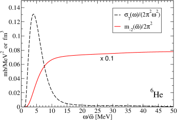
In Ref. Moro an evaluation of the experimental number for the polarizability of 6He was presented, leading to fm3. This was obtained from the inverse energy weighted integral of experimental and theoretical response functions for 6He. The experimental distribution was measured by Aumann et al. Aumann from the Coulomb breakup of 6He on Lead and Carbon at 240 MeV/ up to 8 MeV above threshold. In order to obtain the polarizability, data were extrapolated up to 12.3 MeV, where the threshold for the breakup into two tritons opens up. The theoretical curve was taken from a calculation of the dipole transition to the continuum Thompson in a three-body model with phenomenological and interactions plus an effective three-body force, also calculated up to the two tritons threshold. The estimate was done in two steps: (i) an average of the experimental data and theoretical curve was taken up to 12.3 MeV; (ii) to account for the higher energies, the polarizability of 4He was added. The latter one basically comes from integrating the photo-dissociation data from Arkatov et al. Arkatov . Because we can access the full response functions using the LIT method at any energy below the pion production threshold, we can verify these two approximations. First, it is interesting to study the convergence of calculated as a sum rule of the response, see Eq. (4) and (5), to investigate the validity of (i). In Fig. 7, we present both the integrand function versus and the convergence of the integral versus . At MeV the sum rule is exhausted only up to 75. Thus only 75 of the is based solely on experimental data. At 12.3 MeV, where the two 3H channel opens up the sum rule is exhausted up to 90. We observe that one needs to integrate up to MeV of energy to have the sum rule exhausted at the level.
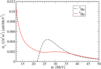
To verify the approximation (ii) we can compare the integrand function for 6He and 4He at energies beyond 12.3 MeV. In Fig. (8) we observe that the two curves agree with each other for MeV, where the sum rule is almost exhausted. In the region beyond the 4He disintegration threshold and below about MeV one would over estimate the sum rule integrating the 4He curve, because one gets 0.044 fm3, to be compared to the 0.027 fm3 obtained when correctly integrating the 6He curve. On the other hand, neglecting the part of the cross section for MeV and below the 4He disintegration threshold one underestimates the sum rule. The contribution of this portion is 0.037 fm3, about 5 of the sum rule. These two effects almost cancel out so that, the approximation (ii) does not lead to a big error.
We think that the main reason of the disagreement between the estimate from Ref. Moro and our calculations comes from the difference in the low-energy part of the response. In our previous work He6Sonia1 ; He6Sonia2 we have shown that our calculations with semi-realistic potentials underestimates the data from Aumann et al. Aumann . Thus, what we observe for the polarizability is consistent with this fact. We would like to point out that (i) nuclear corrections might affect the results in the ion scattering experiment of Aumann and that (ii) as discussed earlier, similar experiments for 3He lead to large discrepancy with photo-dissociation results. Nevertheless, measuring from the dipole response function it would be desirable to have data up to higher energies than 12.3 MeV. Additional or alternative measurements of would help to better constrain this observable.
V Conclusions
We summarize our results as follows. We have carried out an estimate of the nuclear polarizability of 6He based on the hyperspherical harmonics expansion with simple semi-realistic potentials. Our calculations clearly reproduce the fact that the polarizability of the halo nucleus of 6He is much larger than that of the tightly bound 4He. For 4He the semi-realistic Minnesota potentials lead to a value of the polarizability which is consistent with realistic calculations and is about 15 smaller than the average value in the experimental band. Nevertheless, a large disagreement is found for 6He. In order to estimate we have chosen a potential that reproduces the separation energy and then we investigated the correlation of the polarizability with the skin radius. Our final result is fm3, which is about a factor of 2 smaller than the estimates from experimental data. This points towards a disagreement of microscopic theory and experiments. To shed light on this, it would be nice to have more data or alternative measurements of . Concerning the theoretical calculations, it is desirable to extend these results to realistic potentials including also three-body forces. We leave this subject to a future work.
VI Acknowledgment
The work of R. Goerke and S. Bacca was supported in part by the Natural Sciences and Engineering Research Council (NSERC) and in part by the National Research Council of Canada. The work of N. Barnea was supported by the ISRAEL SCIENCE FOUNDATION (grant no. 954/09). Numerical calculations were performed at TRIUMF.
References
- (1) K. Pachucki, A.M. Moro, Phys. Rev. A 75, 032521 (2007).
- (2) A. Tamii et al., Phys. Rev. Lett. 17, 062502 (2011).
- (3) W. Nöerterhäuser et al., Phys. Rev. A 83, 012516 (2011).
- (4) L. B. Wang et al., Phys. Rev. Lett. 93, 142501 (2004).
- (5) M. Brodeur et al., Phys. Rev. Lett. 108, 052504 (2012).
- (6) P. Mueller et al., Phys. Rev. Lett. 99, 252501 (2007).
- (7) A. Antognini et al., Can. J. Phys. 89, 47 (2011).
- (8) F. Goeckner, L. O. Lamm, and L. D. Knutson, Phys. Rev. C 43, 66 (1991).
- (9) I. Stetcu, S. Quaglioni, J.L. Friar, A.C. Hayes, and P. Navratil, Phys. Rev. C 79, 064001 (2009).
- (10) I. Tanihata, J. Phys. G 22, 157 (1996).
- (11) N. Barnea and A. Novoselsky, Phys. Rev. A 57, 48 (1998); Ann. Phys. (N.Y.) 256, 192 (1997).
- (12) N. Barnea, W. Leidemann, and G. Orlandini, Phys. Rev. C 61, 054001 (2000); Nucl. Phys. A693, 565 (2001).
- (13) V.D. Efros, W. Leidemann, and G. Orlandini, Phys. Lett. B338, 130 (1994).
- (14) E. Dagotto, Rev. Mod. Phys. 66, 763 (1994), and references therein.
- (15) S. Bacca, M. A. Marchisio, N. Barnea, W. Leidemann and G. Orlandini, Phys. Rev. Lett. 89, 052502 (2002).
- (16) S. Bacca, N. Barnea, W. Leidemann and G. Orlandini, Phys. Rev. C 69, 057001 (2004).
- (17) M. A. Marchisio, N. Barnea, W. Leidemann, and G. Orlandini, Few-Body Syst. 33, 259 (2003).
- (18) V.D. Efros, W. Leidemann, and G. Orlandini, Few-Body Syst. 26, 251 (1999); D. Andreasi, W. Leidemann, C. Reiss, and M. Schwamb, Eur. Phys. J. A24, 361 (2005).
- (19) D.R. Thompson, M. LeMere and Y.C. Tang, Nucl. Phys. A286, 53 (1977).
- (20) R. A. Malfliet and J. A. Tjon, Nucl. Phys. A127, 161 (1969).
- (21) S.C. Pieper, and R.B. Wiringa, Phys. Rev. Lett. 89 (2002) 182501.
- (22) I. Brida and F.M. Nunes, Nucl. Phys. A 847, 1 (2010).
- (23) G. Papadimitriou, A. T. Kruppa, N. Michel, W. Nazarewicz, M. Ploszajczak and J. Rotureau, Phys. Rev. C 84, 051304 (2011).
- (24) D. Gazit, N. Barnea, S. Bacca, W. Leidemann, and G. Orlandini, Phys. Rev. C 74, 061001 (2006).
- (25) J. L. Friar, Phys. Rev. C 16, 1540 (1977).
- (26) Yu.M. Arkatov, P.I. Vatset, V.I. Voloshuchuk, V.A. Zolenko, abnd I.M. Prokhorets, Yad. Phyz. 31, 1400 (1980) [Sov. J. Nucl. Phys. 31, 726 (1980)].
- (27) Yu.M. Arkatov, et al., Yad. Phyz. 19, 1172 (1974) [Sov. J. Nucl. Phys. 19, 598 (1974)].
- (28) J. Piekarewicz, B. K. Agrawal, G. Coló, W. Nazarewicz, N. Paar, P.-G. Reinhard, X. Roca-Maza, and D. Vretenar, Phys. Rev. C 85, 041302 (2012).
- (29) S. Shlomo and M. R. Anders, private communication.
- (30) S. Bacca, N. Barnea, A. Schwenk, arXiv:1202.0516.
- (31) I. Tanihata, D. Hirata, T. Kobayashi, S. Shimomura, K. Sugimoto and H. Toki, Phys. Lett. B 289, 261 (1992).
- (32) G. D, Alkhazov, et al., Phys. Rev. Lett. 78, 2313 (1997).
- (33) O. A. Kislev, et al., Eur. Phys. J. A 25, 215 (2005).
- (34) T. Aumann et al., Phys. Rev. C 59, 1252 (1999).
- (35) I.J. Thompson, B.V. Danilin, V.D. Efros, J.S. Vaagen, J.M. Bang, and M.V. Zhukov, Phys. Rev. C 61, 024318 (2000).
