Bouchaud-Mézard model on a random network

Abstract

We studied the Bouchaud-Mézard(BM) model, which was introduced to explain Pareto’s law in a real economy, on a random network. Using ”adiabatic and independent” assumptions, we analytically obtained the stationary probability distribution function of wealth. The results shows that wealth-condensation, indicated by the divergence of the variance of wealth, occurs at a larger $J$ than that obtained by the mean-field theory, where $J$ represents the strength of interaction between agents. We compared our results with numerical simulation results and found that they were in good agreement.

I Introduction

Researchers in the field of complex networks agree that a change in the network topology induces a critical change in dynamics. Pastor-Satorras and Vespignani first showed the absence of an epidemic threshold in a scale-free networkPastor-Satorras2001 , following which many researchers have focused on the dynamics on complex networks, such as synchronizationNishikawa2003 ; Ichinomiya2004 , pattern formationNakao2008 , and other phenomena.

In this study, we focus on the Bouchaud-Mézard(BM) model on a complex networkBouchaud2000 . It is known that the wealth distribution in a real economy exhibits a power-law behavior, called Pareto’s lawPareto . With a view to this power law, Bouchaud and Mézard proposed a model, given by the following Stratonovich stochastic differential equation.

$$dx_{i}=\frac{J}{N}\sum_{j=1}^{N}(x_{j}-x_{i})dt+\sqrt{2}\sigma x_{i}\circ dW_{i},$$ (1)

where $x_{i}$, $N$, $J$, and $\sigma^{2}$ represent the wealth of the $i$-th agent, number of agents, coupling between agents, and variation of noise, respectively. In this model, the evolution of the wealth is determined by two processes: exchange of wealth and a random multiplicative process, respectively described by the first and second term in the right-hand side of Eq.(1). Bouchaud and Mézard analyzed this model using the mean-field theory and calculated the probability density function(PDF) of wealth. They showed that the stationary distribution of normalized wealth $x_{i}/\langle x\rangle$, where $\langle\cdots\rangle$ represents the average over all agents, exhibits the power-law behavior. They also found that “wealth-condensation,” which is indicated by the divergence of the variance of $x_{i}/\langle x\rangle$, occurs at $J\leq J_{c}=\sigma^{2}$. The divergence of the variance implies that wealth condenses to a few rich agents. On the other hand, if $J>J_{c}$, the variance remains finite, and the wealth of many agents is close to the average.

In the original BM model, all agents are coupled with each other. However, in a real economy, agents can exchange their wealth with a limited number of agents. Therefore, it is natural to extend the BM model on a complex network in which the number of neighbors is limited. Some studies have already dealt with this subject. In their original study on the BM-modelBouchaud2000 , Bouchaud and Mézard carried out numerical simulations on a regular random graph to estimate the exponent of the power-law behavior. They reported that the exponent obtained from numerical simulation becomes smaller than that obtained from mean-field theory. Some studies have also reported on the simulation of this model on a Barabási-Albert (BA) network and a Watts-Strogatz(WS) networkGarlaschelli2004 ; Souma2001 . In these studies, the authors discussed numerical simulation results, however, none of them proposed a quantitative theory that could explain these results.

This study aims to develop a quantitative theory of the BM model on a random network. The key assumption of our theory is ”adiabatic and independent” assumptions on the stationary distribution function, which is explained in a later section. By using these assumptions and the central limit theorem, we analytically derive the equations that determine the stationary distribution function in the non-wealth-condensate phase. We compared our analytic results with those of the numerical simulation, and we found that our theory showed better agreement than did the mean-field theory.

The remainder of this paper is organized as follows. In the next section, we define the model we investigate in this paper. Then, we describe our theory and its results, first for the case of a regular random network and then for a random network with arbitrary degree distribution. In Sec. IV, we describe a comparison of our analysis and the numerical simulation. In the last section, we summarize our results and discuss the problem to be solved.

II Model

The original BM model is expressed using the Stratonovich stochastic differential equation; however, we use the equivalent Ito stochastic equation for mathematical convenience. We consider the BM model on a complex network described by the following Ito stochastic differential equations

$${dx_{i}}=[J\sum_{j=1}^{N}a_{ij}(x_{j}-x_{i})]dt+\sqrt{2}\sigma x_{i}dW_{i},$$ (2)

where $x_{i}$, $J$, $N$, and $\sigma^{2}$ are the same as Eq.(1), and $a_{ij}$ represents the adjacent matrix. On the network model, we consider a random network in which the degree distribution is given by $Q(k)$.

III Theory

In this section, we consider the stationary PDF of the normalized wealth of Eq.(2). Eq.(2) is invariant under the change of scale $x_{i}^{\prime}=\alpha x_{i}$ for any positive constant $\alpha$, and we can assume $\langle x\rangle=1$ without loss of generality. We derive the analytic form of the stationary PDF of $x_{i}/\langle x\rangle$, the normalized wealth at node $i$. First, we explain our method on the regular random graph, in which all nodes have the same degree $k$. Then, we extend the analysis to the general random network model, whose degree distribution is given by $Q(k)$.

III.1 Case of a regular random network

This subsection focuses on the analysis of the system when each node has the same degree $k$, in other words, $Q(k)$ is a delta function. We assume that $\rho_{i}(x,t)$, the PDF of wealth at node $i$, is independent of $i$, $\rho_{i}(x,t)=\rho(x,t)$.

First, we review the mean-field treatment of the BM model. We consider the distribution of wealth at node $i$. By using the mean-field theory, we approximate $\frac{1}{k}\sum_{j}a_{ij}x_{j}=\langle x\rangle=1$ in Eq. (2). Under this approximation, $\rho(x,t)$ satisfies the following Fokker-Planck equation,

$$\frac{\partial\rho}{\partial t}=-\frac{\partial}{\partial x}\left[(Jk(1-x)-\sigma^{2}x)\rho\right]+\sigma^{2}\frac{\partial}{\partial x}\left[x\frac{\partial}{\partial x}(\rho x)\right]$$ (3)

and we find $\rho^{MF}_{eq}(x)$, the stationary PDF obtained from this equation, as

$$\rho^{MF}_{eq}(x)=C\exp(-\alpha/x)x^{-2-\alpha},$$ (4)

where $\alpha=Jk/\sigma^{2}$ and $C=\alpha^{1+\alpha}/\Gamma(1+\alpha)$. In this case, wealth-condensation, defined as the divergence of $\langle x^{2}\rangle$, occurs at $Jk\leq\sigma^{2}$.

To proceed beyond the mean-field approximation, we make what we call “adiabatic and independent” assumptions. We define the ”local” field $\tilde{x}_{i}=\frac{1}{k}\sum_{j}a_{ij}x_{j}$. Because $a_{ij}$ is not 0 only if nodes $i$ and $j$ are connected, $\tilde{x}_{i}$ represents the local average of the wealth around node $i$.

If $\tilde{x}_{i}$ is fixed, the PDF of $x$ at node $i$ is given by solving the ”local” Fokker-Planck equation

$$\frac{\partial\rho}{\partial t}=-\frac{\partial}{\partial x}\left[Jk(\tilde{x}_{i}-x)\rho-\sigma^{2}x\rho\right]+\sigma^{2}\frac{\partial}{\partial x}\left[x\frac{\partial}{\partial x}(\rho x)\right],$$ (5)

and the conditional PDF of $x$ under the local field $\tilde{x}$ is given by

$$\rho_{eq}(x|\tilde{x})=C(\tilde{x})\exp(-\alpha\tilde{x}/x)x^{-2-\alpha},$$ (6)

where $C(\tilde{x})=(\alpha\tilde{x})^{1+\alpha}/\Gamma(1+\alpha)$.

Here we make the “adiabatic and independent” assumptions. First, we assume the static PDF $\rho_{eq}(x)$ can be approximated by

$$\rho_{eq}(x)=\int d\tilde{x}P(\tilde{x})\rho_{i}(x|\tilde{x}),$$ (7)

where $P(\tilde{x})$ is the PDF of $\tilde{x}$. If $\tilde{x}$ changes much slower than $x$, this condition is satisfied, and therefore we call it the “adiabatic” assumption. Under this assumption, the problem to calculate $\rho_{eq}(x)$ is reduced to the one to calculate $P(\tilde{x})$.

The second assumption is needed to calculate $P(\tilde{x})$. We assume that the random variables $x_{j}$, where $j$ runs in the neighborhood of node $i$, are independent. This assumption enables us to use the central limit theorem to obtain $P(\tilde{x})$. We consider the case in which the variance of $x$ is finite, and that the average and variance of $x$ are 1 and $s^{2}$, respectively. Using the central limit theorem, we can approximate

$$P(\tilde{x})\sim\frac{\sqrt{k}}{\sqrt{2\pi}s}\exp\left(-\frac{k(\tilde{x}-1)^{2}}{2s^{2}}\right).$$ (8)

Inserting Eq. (8) into Eq. (7), we obtain

$$\rho_{eq}(x)\sim\int_{0}^{\infty}d\tilde{x}\frac{\sqrt{k}}{\sqrt{2\pi}s}\exp\left(-\frac{k(\tilde{x}-1)^{2}}{2s^{2}}\right)\rho_{eq}(x|\tilde{x}).$$ (9)

The final step is to check that $\langle x\rangle=1$ and to calculate $s^{2}$. Using $\int_{0}^{\infty}dx\rho_{eq}(x|\tilde{x})x=\tilde{x}$ and $\int_{0}^{\infty}dx\rho_{eq}(x|\tilde{x})x^{2}=\frac{\alpha}{\alpha-1}\tilde{x}^{2}$ for $\alpha>1$, we obtain

$$\int x\rho_{eq}(x)=\int_{0}^{\infty}d\tilde{x}P(\tilde{x})\tilde{x}\sim\int_{-\infty}^{\infty}\tilde{x}P(\tilde{x})d\tilde{x}=1,$$ (10)

and

$$\int x^{2}\rho_{eq}=\int_{0}^{\infty}d\tilde{x}\frac{\alpha}{\alpha-1}\tilde{x}^{2}P(\tilde{x})\sim\frac{\alpha}{\alpha-1}\left(1+\frac{s^{2}}{k}\right).$$ (11)

Here we change the lower limit of integration from 0 to $-\infty$, assuming $k/s^{2}$ to be large. From Eq.(10), we conclude that $\langle x\rangle=1$ , and that there is no inconsistency. From Eqs. (10) and (11), the variation of $x$ is given by $\frac{1}{\alpha-1}(\frac{\alpha s^{2}}{k}+1)$. Therefore we find the self-consistency condition for $s^{2}$ as

$$[(k-1)\alpha-k]s^{2}=k.$$ (12)

Eqs.(6), (9), and (12) are the set of equations that determine $\rho_{eq}(x)$.

We should make several comments on these results. First, this theory gives a distribution that does not obey the power-law behavior. Eq.(9) shows that the PDF $\rho_{eq}(x)$ is written with the integral of $P(\tilde{x})\rho_{eq}(x|\tilde{x})$ over $\tilde{x}$. Because $P(\tilde{x})$ is Gaussian, $\rho_{eq}(x)$ does not exhibit the simple power-law behavior.

The next important suggestion of this theory concerns the wealth-condensation transition. In our theory, $s^{2}$ diverges if $(k-1)\alpha-k=0$, implying that the wealth-condensation occurs at this point. Using $\alpha=Jk/\sigma^{2}$, this leads to the conclusion that wealth condensation occurs at $J_{c}=\sigma^{2}/(k-1)$. On the other hand, the mean-field theory gives the divergence of the variance at $J_{c}=\sigma^{2}/k$. Therefore the difference between our theory and the mean-field theory can be tested by estimating $J_{c}$ from the simulation.

Finally, we note that our theory can be applied only for the non-wealth-condensation phase. We need the central limit theorem to obtain $P(\tilde{x})$, which is only applicable for the case in which the variance of $x$ is finite. We discuss this point in greater detail in the final section.

III.2 Case of a general random network

In this subsection, we extend the developed method for a regular random graph to a general random network.

As in the case of a regular random network, we start from the mean-field theory. In this theory, we define $\rho_{k}(x,t)$ as the PDF of $x$ on the node whose degree is $k$. Because this network is heterogeneous, the mean of $x$ may depend on $k$. Therefore, we need to define $\bar{x}_{k}=\int dxx\rho_{k}(x,t)$, the average of $x$ on nodes with degree $k$, to perform the mean-field calculation. The mean-field Fokker-Planck equation is constructed in the same manner as in the case of the SIS model or Kuramoto oscillatorPastor-Satorras2001 ; Ichinomiya2004 , and we obtain

$$\frac{\partial\rho_{k}(x,t)}{\partial t} = -\frac{\partial}{\partial x}\left[J\sum_{k^{\prime}}\frac{kk^{\prime}Q(k^{\prime})}{\langle k\rangle}(\bar{x}_{k^{\prime}}-x)\rho_{k}(x,t)\right.$$

$$- \left.\sigma^{2}x\rho_{k}(x,t)\right]+\sigma^{2}\frac{\partial}{\partial x}\left[x\frac{\partial}{\partial x}(x\rho_{k}(x,t))\right]$$

We can simplify this equation by introducing the “weighted” average of $x$ as $\bar{x}=\sum_{k}\frac{kQ(k)}{\langle k\rangle}\bar{x}_{k}$, which leads to

$$\frac{\partial\rho_{k}}{\partial t}=-\frac{\partial}{\partial x}[Jk(\bar{x}-x)\rho_{k}-\sigma^{2}x\rho_{k}]+\sigma^{2}\frac{\partial}{\partial x}\left[x\frac{\partial}{\partial x}(x\rho_{k})\right],$$ (14)

where we abbreviated $\rho_{k}(x,t)$ as $\rho_{k}$. As in the case of a regular random graph, we obtain $\rho^{MF}_{eq,k}(x)$, the stationary PDF by the mean-field theory, as

$$\rho^{MF}_{eq,k}(x)=C_{k}(\bar{x})\exp(-\alpha_{k}\bar{x}/x)x^{-2-\alpha_{k}},$$ (15)

where $\alpha_{k}=Jk/\sigma^{2}$ and $C_{k}(\bar{x})=(\alpha_{k}\bar{x})^{1+\alpha_{k}}/\Gamma(1+\alpha_{k})$. Finally, $\bar{x}$ is determined to satisfy the condition $\langle x\rangle=1$. From $\int dxx\rho^{MF}_{eq,k}(x)=\bar{x}$, we obtain $\bar{x}=1$.

Now we follow the same procedure as that described in the previous subsection to calculate the PDF more accurately. We consider the PDF of the wealth on node $i$, whose degree is $k$. If the average of sums of $x$ in the neighborhood of node $i$ is given by $\tilde{x}$, we find the conditional PDF of $x$ on node $i$ as

$$\rho_{k}(x|\tilde{x})=C_{k}(\tilde{x})\exp(-\alpha_{k}\tilde{x}/x)x^{-2-\alpha_{k}},$$ (16)

Using the adiabatic assumption explained in the previous subsection, we assume

$$\rho_{k}(x)=\int d\tilde{x}P_{k}(\tilde{x})\rho_{k}(x|\tilde{x}).$$ (17)

Next, we approximate $P_{k}(\tilde{x})$ by Gaussian using the independent assumption. One difference between the regular random graph and the random graph with arbitrary degree distribution lies in that we need to assume Lindeberg’s condition in this case. Suppose that there are independent variables $y_{1},\cdots y_{m}$ , whose mean and variance are $\mu_{1},\mu_{2},\cdots\mu_{m}$ and $s_{1}^{2},s_{2}^{2},\cdots s_{m}^{2}$ respectively. Then, the PDF of $\frac{1}{m}(y_{1}+y_{2}+\cdots y_{m})$ converges to the Gaussian, whose mean and variance are $\frac{1}{m}(\mu_{1}+\mu_{2}+\cdots+\mu_{m})$ and $\frac{1}{m^{2}}(\sigma_{1}^{2}+\sigma_{2}^{2}+\cdots\sigma_{m}^{2})$, for $m\rightarrow\infty$, if Lindeberg’s condition is satisfiedGnedenko . Although $m$ is finite in our case, we can approximate

$$P_{k}(\tilde{x})\sim\frac{1}{\sqrt{2\pi}S_{k}}\exp\left(-\frac{(\tilde{x}-1)^{2}}{2S_{k}^{2}}\right),$$ (18)

where $S_{k}^{2}$ is a parameter that must be determined by the self-consistency condition.

The final step is to obtain self-consistent equations for the mean and variance of $x_{k}$. Using $\int dxx\rho_{k}(x)=1$ and $\int dxx^{2}\rho_{k}(x)=\frac{\alpha_{k}}{\alpha_{k}-1}(1+S_{k}^{2})$ obtained from Eqs.(16), (17) and (18), we respectively obtain $\mu_{k}$ and $s_{k}^{2}$, the average and variance of $x$ on nodes with degree $k$, as $\mu_{k}=1$ and

$$s_{k}^{2}=\frac{\alpha_{k}S_{k}^{2}+1}{\alpha_{k}-1}.$$ (19)

A node with degree $k$ is connected to a node whose degree is $k^{\prime}$ with probability $\frac{kk^{\prime}Q(k^{\prime})}{\langle k\rangle}$, and we obtain

$$S_{k}=\frac{1}{k^{2}}\sum_{k^{\prime}}\frac{kk^{\prime}Q(k^{\prime})}{\langle k\rangle}{s_{k^{\prime}}}^{2}=\frac{u}{k},$$ (20)

where $u$ represents the weighted average of the variance,

$$u=\sum_{k}kQ(k)s_{k}^{2}/\langle k\rangle.$$ (21)

From Eqs.(19) and (20), we obtain

$$s_{k}^{2}=\frac{\alpha_{k}u/k+1}{\alpha_{k}-1}.$$ (22)

Inserting this equation into Eq.(21), we obtain

$$u=\sum_{k}\frac{Q(k)}{\langle k\rangle}\frac{\alpha_{k}u+k}{\alpha_{k}-1},$$ (23)

which leads to our final result,

$$\left(1-\sum_{k}\frac{Q(k)\alpha_{k}}{\langle k\rangle(\alpha_{k}-1)}\right)u=\sum_{k}\frac{Q(k)k}{\langle k\rangle(\alpha_{k}-1)}$$ (24)

Eqs.(16), (17), (18), (20), and (24) are the set of equations that determine the stationary PDF.

The most important difference between the mean-field theory and ours lies in that there is no effect of $Q(k)$ in the mean-field theory. In the mean-field theory, the PDF on the node with degree $k$ given by Eq.(15) does not depend on $Q(k)$, which causes a curious behavior. Suppose that we decrease $J$ from a large value to 0. At $J=\sigma^{2}/k$, the node with degree $k$ goes into the wealth-condensate phase, whereas nodes with a larger degree do not condensate. Therefore, the mean-field theory predicts the coexistence of condensated and non-condensated nodes. In this theory, low-degree nodes condensate at large $J$, whereas high-degree nodes do not condensate until $J$ becomes sufficiently small.

On the other hand, all PDFs with different degrees are connected through $u$ in our theory. In this theory, $u$ diverges when $\sum_{k}\frac{Q(k)\alpha_{k}}{\langle k\rangle(\alpha_{k}-1)}=1$, which implies the divergence of all $s_{k}$ from Eq.(22). In our theory, wealth-condensation occurs on all nodes simultaneously.

Finally, we comment on the behavior of the BM model on a scale-free network. Researchers in the field of complex networks may consider that a singular behavior occurs in a scale-free network upon the wealth-condensation transition, such as the divergence or disappearance of the transition point $J_{c}$. Unfortunately,this is not the case. The main difference between our case and other models that show singularity, such as the SIS-model or Kuramoto transition, lies in that we impose the self-consistency condition on the variance of $x$, and not on its average. As shown in Eq.(20), we divide the weighted average of the variance $s_{k}^{2}$ by $k$ to calculate $S_{k}$. This eliminates the singular behavior that we often observe in the dynamics on a scale-free network.

IV Simulation

In this section, we test the analytic results obtained in the previous section by comparing them with numerical simulations.

Because we have presented two analytic results, one for a regular random network and the other for a heterogeneous random network, we carried out the simulations for both networks. For the former, all nodes had the same degree, whereas for the latter, half of the nodes had degree 10 and the other half had degree 20.

We use these two models because it is easy to calculate the PDF in these models. However, the readers might find these models too artificial. To test our theory in a more realistic model, we show the result of simulations on BA-networkBarabasi1999 . Here we note that the direct calculation of wealth distribution is rather hard because we must calculate integral in Eq.(17) for many values of $k$. In this paper, we investigate $s_{k}^{2}$, the variation of $x$ at a node with degree $k$ to test our theory instead, because it is much easier to compute.

In the following simulation, we carried out numerical integration by the Euler-Maruyama algorithm to obtain the distribution of normalized wealth $x/\langle x\rangle$.

IV.1 Case of a regular random network

In this subsection, we show the simulation result for a regular random network and compare it with our theory.

First we calculate the PDF of the normalized wealth from 10 simulation trials on networks that include 5000 nodes. In Fig.1, we show the obtained PDF for the network with degree $k=10$, $\sigma^{2}=1$ and coupling $J=0.3$, 0.4, and 0.5. For all $J$, the distribution coincides well with our theory, indicated by the solid line. The PDF given by the mean-field theory, indicated by the dashed line, strongly underestimates the probability density at small $x/\langle x\rangle$. On the other hand, our theory gives a slightly larger PDF than the simulation, although, it shows better agreement.

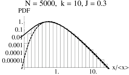
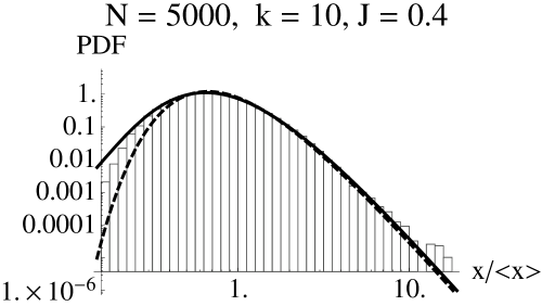
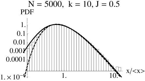
Figure 1: Log-log plot of PDF of normalized wealth obtained by simulation when $k=10$, $\sigma^{2}=1$, and $J=0.3,0.4$, and 0.5. The solid and dashed lines indicate the result obtained by our theory and that obtained by the mean-field theory,respectively.

Here we investigate the temporal and spatial correlation of $x$ to test the “adiabatic and independent” assumptions used to derive Eqs.(7) and (9). In the right-hand side of Fig.2, we plot the typical trajectory of $x(t)$ and $\tilde{x}(t)$. Because the model we study is described by stochastic differential equations, it is difficult to show that the change in $\tilde{x}_{i}$ is “slower” than that in $x_{i}$, however, it seems that $x_{i}$ changes more quickly than $\tilde{x}_{i}$. Concerning the “independent” assumption, we show the scatter plot between $x$ and $\tilde{x}$ in the left-hand side of Fig.2. Although there exists a tendency for $x$ to increases as $\tilde{x}$ increases, it is not strong. The correlation between $x$ and $\tilde{x}$ calculated by the numerical simulation is 0.238. Therefore we conclude that the “adiabatic” “independent” assumptions are fairly good.

Figure 2: Temporal and spatial behavior of $x$. Left: time series of $x$ and $\tilde{x}$ at one node. Right: scatter plot of $x$ and $\tilde{x}$. Both plots are obtained from the simulation at $N=5000$, $k=10$ and $J=0.3$.

In Fig. 3, we show the PDF at $J=0.5$, $\sigma^{2}=1$ and $k=4,10$, and 20. It is clear that the discrepancy between our theory and the numerical simulation increases as $k$ decreases. This is not surprising, because the error caused by the application of the central limit theorem increases at small $k$. However, our theory appears to be better than the mean-field theory, even in the worst case. For example, when $k=4$, the probability density obtained by the mean-field theory is smaller than $10^{-5}$ at $x=0.1$, whereas the numerical simulation and our theory shows that it is $O(10^{-1})$. On the other hand, the difference from the result of numerical simulation at large $x$ is indistinguishable between our theory and mean-field theory.

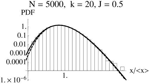
Figure 3: Log-log plot of PDF obtained by simulation when $J=0.5$, $\sigma^{2}=1$ and $k=4,10$, and 20. The solid and dashed lines indicate the result obtained by our theory and that obtained by the mean-field theory, respectively .

Finally, we check the wealth-condensation transitions. Though our theory does not exhibit the exact power-law behavior, it suggests that variance of normalized wealth diverges at $J_{c}=\sigma^{2}/(k-1)$. Therefore, we can expect power law behavior $\rho(x)\propto x^{-3}$ for large $x$ at this point. On the other hand, the mean-field approximation gives $J_{c}=\sigma^{2}/k$, and we can test our theory by estimating $J_{c}$ by checking the exponential tail. In Fig.4 we plot the exponent $\gamma$, $\rho(x)\propto x^{-\gamma}$ at $x\gg 1$, estimated from the fitting of the PDF obtained through 100 simulation trials on a regular random graph $N=1000$, $k=4$. It is clear that wealth-condensation occurs at $J\sim 0.35$, which is closer to the prediction of our theory $J_{c}=0.33$, than that of the mean-field theory , $J_{c}=0.25$.

Figure 4: Exponent obtained by simulation for $k=4$, $\sigma^{2}=1$. The dotted line indicates the wealth-condensation transition.

IV.2 Case of a heterogeneous network

In this section, we present the simulation result for a heterogeneous network. As explained in Sec.III, the PDF $\rho_{eq,k}(x)$ does not depend on $Q(k)$ in the mean-field approximation. In this approximation, the PDF of the wealth for nodes whose degree is $k$ equals that for the regular random graph. On the other hand, our theory predicts that the PDF changes if $Q(k)$ differs. To test our theory for heterogeneous network, we make the network that half of the node have degree $k_{1}=10$, and other half have degree $k_{2}=20$.

The PDF of the normalized wealth obtained by the simulation is shown in Fig.5 for $J=0.3$ and $\sigma^{2}=1$. In this figure, we also plot the PDF obtained by our theory for a heterogeneous network and a regular random graph with degree $k_{1}$ or $k_{2}$ and by the mean-field theory and that by our theory for regular random graph with degree $k_{1}$ or $k_{2}$. For the PDF on nodes with degree 10, the PDF obtained by our theory, indicated by the solid line, is suppressed at small $x$ compared with the case of a regular random network, indicated by the dashed line. The PDF obtained by the simulation shows better agreement with our theory for a heterogeneous network. For the PDF on node with degree 20, the difference among the three theories is small; however, we can conclude that our theory can estimate the PDF very well.

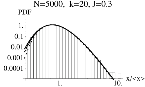
Figure 5: PDF obtained from numerical simulation on a heterogeneous network. The solid, dashed, and dotted lines indicate the PDF obtained by our theory for a heterogeneous network and a regular random graph, and by the mean-field theory, respectively

IV.3 Case of BA-network

To test our theory in a more realistic network model, we show the simulation result on the BA-network model. The PDF obtained from simulations on a BA-model with minimum degree 4, $J=0.3$ and $\sigma^{2}=1$ is given in the left-hand side of Fig.6. As we have noticed, it is slightly difficult to show the PDF obtained from our theory. Instead of the PDF, we plot the $s^{2}_{k}$, the variation of $x$ on nodes whose degree is $k$, obtained by simulation and that obtained by Eq. (22), in the right-hand side of Fig. 6 . The theoretical prediction, indicated by the thick line, coincide well with the result of numerical simulation.

Figure 6: Result of simulation for BA-network with minimum degree 4 and $J=0.3$, $\sigma^{2}=1.0$. Left: PDF. Right: $s_{k}^{2}$, the variation of $x$ on nodes with degree $k$. Thick line indicates the theoretical result obtained from Eq.(22).

V Summary

In this paper, we derived the PDF of the Bouchaud-Mézard model on a random network. Using adiabatic and independent assumptions, we derived the equations for the PDF, Eqs. (6), (9), and (12) for a regular random network, and Eqs.(16), (17), (18), (20), and (24) for a general random graph. It is difficult to solve these equations analytically; however, doing so provides considerable information about the wealth-distribution. In particular, we can analytically obtain the wealth-condensation point $J_{c}$ for a regular random graph. These analytic results are compared with the numerical simulations in Sec. IV, and good agreement is found with our theory. Below, we discuss the problem to be solved.

First, we note that the approach we have used in this paper cannot be applied to a wealth-condensate phase. We use the central limit theorem to derive the equation for a stationary PDF; however, this approach is not applicable when the variance of $\rho(x)$ diverges. To treat the wealth-condensate phase, we need a generalized central limit theorem that is applicable when the variance diverges. It is known that the PDF of the sum of independent identical random variables converges to a stable distribution function when the variance divergesGnedenko . It would be possible to make the theory for the wealth-condensate phase on a regular random network using this theorem; however, further work will be required toward this end. For a general random network, the generalized central limit theorem unfortunately remains still insufficient. To treat such a network , we require a generalized central limit theorem for non-identical independent random variables, which has not been yet established.

Second, one might be interested in better approximating the the PDF. As shown in Fig. 3, the PDF obtained by our method still has a large discrepancy with the numerical simulation, especially for nodes with small degree. To reduce these errors, we need to use the improved central limit theorem, which can deal with the rate of convergence. The application of Chebyshev’s rate-of-convergence theoremChebyshev would lead to a better approximation.

Finally, we should comment on the “adiabatic and independent” assumptions. We have no proof to verify these assumptions; however, the coincidence with the simulations suggests that these assumptions work very well. If so, the theory developed in this study will be applicable to other dynamical systems. The essential part of our theory is to impose the self-consistency condition on the average and variance of the dynamical variables on each node. In the case of the BM model, the self-consistency condition for the average is automatically satisfied, and we need only to calculate the variance. This procedure is very general, and it will be applicable to analyze other dynamical behaviors such as synchronization or diffusion.

- (1) R. Pastor-Satorras and A. Vespignani, Phys. Rev. Lett. 86, 3200(2001).
- (2) T. Nishikawa, A. E. Motter, Y.-C Lai, and F. C. Hoppensteadt, Phys. Rev. Lett. 91,014101(2003).
- (3) T. Ichinomiya, Phys. Rev. E 70 026116(2004).
- (4) H. Nakao and A. Mikhaikov, Nature Phys. 6 544(2010).
- (5) J. Bouchaud and M. Mézard, Physica A 282 536 (2000).
- (6) V. Pareto, Cours d’économie politique Macmillan, London 1897.
- (7) D. Garlaschelli, M. I. Loffredo, Physica A. 338 113(2004).
- (8) W. Souma, Y. Fujiwara, and A. Aoyama, cond-mat/0108482.
- (9) D. Garlaschelli and M. I. Loffredo, J. Phys. A 41 224018(2008).
- (10) B. V. Gnedenko and A. N. Kolmogorov, Limit distributions for sums of independent random variables, Addison-Wesley, 1954.
- (11) A.-L. Barabási and R. Albert, Science 286 509(1999).
- (12) P. L. Chebyshev, Acta. Math. 14 305(1890).