The interpretation of Rotation Measures in the presence of inhomogeneous foreground screens

Abstract

We analyze the redshift evolution of the Rotation Measure (RM) in Taylor et al. (2009) dataset, which is based on NVSS radio data at 21 cm, and compare with results from our previous work (Kronberg et al., 2008; Bernet et al., 2008, 2010), based on RMs determined at lower wavelengths, e.g. 6 cm. We find that, in spite of the same analysis, Taylor’s dataset produces neither an increase of the RM dispersion with redshift as found in Kronberg et al. (2008), nor the correlation of RM strength with MgII absorption lines found in Bernet et al. (2008). We develop a simple model to understand the discrepancy. The model assumes that the Faraday Rotators, namely the QSO’s host galaxy and the intervening MgII host galaxies along the line of sight, contain partially inhomogeneous RM screens. We find that this leads to an increasing depolarization towards longer wavelengths and to wavelength dependent RM values. In particular, due to cosmological redshift, observations at fixed wavelength of sources at different redshift are affected differently by depolarization and are sensitive to different Faraday active components. For example, at 21 cm the polarized signal is averaged out by inhomogeneous Faraday screens and the measured RM mostly reflects the Milky Way contributions for low redshift QSOs, while polarization is relatively unaffected for high redshift QSOs. Similar effects are produced by intervening galaxies acting as inhomogeneous screens. Finally, we assess the performance of Rotation Measure synthesis on our synthetic models and conclude that the study of magnetic fields in galaxies as a function of cosmic time will benefit considerably from the application of such a technique, provided enough instrumental bandwidth. For this purpose, high frequency channels appear preferable but not strictly necessary.

1. Introduction

Faraday Rotation Measures (RM) is one of the very few methods to probe extragalactic magnetic fields. The RM is given by the change in observed polarization angle, $\Delta\chi_{0}$, over a change in the observed wavelength square, $\Delta\lambda_{0}^{2}$. For a polarized radio source at cosmological redshift $z_{s}$ it is defined as

$$RM(z_{s})=\frac{{\Delta\chi_{0}}}{{\Delta\lambda_{0}^{2}}}=8.1\cdot 10^{5}\int\limits_{z_{s}}^{0}\frac{n_{e}(z)B_{\parallel}(z)}{(1+z)^{2}}\frac{dl}{dz}dz,$$ (1)

where the RM is in units of rad m^-2, the free electron number density, $n_{e}$, is in cm^-3, the magnetic field component along the line of sight, $B_{\|}$, is in Gauss, and the comoving path increment per unit redshift, $dl$/$dz$, is in pc. Eq. 1 assumes a uniform RM screen across the source and a spatial separation of the linearly polarized source and the Faraday rotating plasma.

In Kronberg et al. (2008) (K08) we used a sample of 268 RM values of extragalactic radio sources to assess the redshift evolution in the RM dispersion. We found an increase in the RM dispersion with redshift, which became statistically significant above $z\sim 1$. We postulated that the increase in the RM dispersion is produced by magnetic fields in intervening galaxies. To test this hypothesis spectra of 71 QSOs at UVES/VLT were taken. In Bernet et al. (2008) (B08) we showed that indeed sightlines with intervening strong MgII absorption systems have significantly higher RM values than those without. The findings in that work implies that $\sim 10\;\mu\rm{G}$ magnetic fields exist in galaxies out to $z\sim 1.3$.

Recently Taylor et al. (2009) (TSS09) determined RM values of 37’543 sources, based on polarization observation of the NRAO VLA Sky Survey (NVSS). After the release of the RM catalogue we compared our RM values with those of TSS09 and found major differences between the two datasets. As we show in section 2.2 using the RM values of TSS09 the results of K08 and B08 can not be reproduced. In this work we present an analysis of the differences found between the two datasets. We then develop a toy model to show that such differences can be accounted for by inhomogeneities in the RM screens of the QSOs host galaxies and intervening galaxies. In view of this model, due to the strong depolarization effects, RM data based on low frequencies observations and interpreted according to Eq. (1) are inadequate to probe inhomogeneous RM screens produced by intervening galaxies.

Recently there has been an increased attention to the effects of inhomogeneous RM screens on the observed degree of polarization and polarization angle as function of wavelength. Rossetti et al. (2008); Mantovani et al. (2009) used multiwavelength radio observations to model depolarization of their sources. They showed that the depolarization as a function of wavelength can be better described including a covering factor for the inhomogeneous screens. Farnsworth et al. (2011) used Westerbork Synthesis Radio Telescope (WSRT) observation at $\sim 1\rm{m}$ combined with NVSS observation at 21 cm to test different depolarization models and RM determination methods. They considered the traditional Faraday dispersion screen (Burn, 1966), a two component model for Faraday Rotation which produces oscillation in the degree of polarization, and the RM Synthesis method. The comparison of the different RM values obtained from these methods revealed that if Faraday structure is present, the different methods may lead to different RMs. They further stress the importance of considering both the polarization angle and amplitude for the correct determination of the RMs.

While several effects may be at work, as briefly discussed in section 2.3, in this paper we keep the level of sophistication of the model to a minimum and focus on the role of Faraday screen particularly on simple ideas associated with inhomogeneity which can account for important observational effects and test these ideas for consistency with available data. The rest of this paper is organized as follows. In section 2 the RM datasets of B08 and K08 are compared and the differences are presented. Previous work on depolarization of extragalactic sources is shortly presented in section 3. In section 4 a depolarization toy model is presented which can account for the differences in the RM values of the two datasets. A discussion of the nature of the partial inhomogeneous RM screens and computed Faraday spectra as comparison for RM surveys is presented in section 5. In section 6 we give a summary of our findings.

2. Rotation Measure Data

2.1. Datasets

The RM values used in K08, B08 and Bernet et al. (2010) were collected by P. Kronberg and collaborators over the past decades using polarization observations at various telescopes, including VLA and Effelsberg. The sample consists of 901 sources with determined RM and redshifts, partly taken by Kronberg and collaborators, partly taken from the literature (Simard-Normandin et al., 1981). Until the work of TSS09 it has been the only existing large RM catalogue. Generally at least three wavelengths were used for the RM determination (Phil Kronberg, private communication) using polarization data between 37 to 0.9 GHz, with the bulk of the data between $\sim$ 10.5 to 1.6 GHz (Simard-Normandin et al., 1981).

In the following sections we will assume that the determinations of the RM values of K08 were typically done at 6 cm and designate the RM values as $\rm{RM_{6}}$. Of course due to the heterogeneity of the sample the wavelength range and typical value over which the RMs are determined might vary. While this is undesirable, its main effect should be the introduction of noise in the relations predicted by our model between measured quantities. There might be additional issues associated with the heterogenous character of the polarization data used for the RM determinations, which, however, are not addressed here.

The sample of K08 consists of 268 sources at Galactic latitudes $|b|>45^{\circ}$ (exact definition given in K08). In B08 we obtained high resolution spectra of 71 relatively bright QSOs and relaxed the selection to $|b|>30^{\circ}$. Here we use the subset that was employed in the study of B08 and Bernet et al. (2010) (the RM data are still proprietary and will be published elsewhere by P. Kronberg), except when we look for differences in the redshift evolution and use all sources at $|b|>30^{\circ}$ which were also in the Taylor et al. (2009) catalogue.

The RM values of TSS09 are based on the NRAO VLA Sky Survey (NVSS) from Condon et al. (1998) which covers the sky at declinations $|\delta|>40^{\circ}$ in Stokes I, Q and U. The survey imaged the sky at 21 cm with a resolution of $\sim 45$ arcsecs and produced a catalogue of $2\times 10^{6}$ discrete sources. TSS09 choose a subsample of this catalogue and derived RM values of these sources based on determination of the polarization angles at 1364.9 MHz and 1435.1 MHz. The subsample was selected by requesting a source intensity $\rm{I}>5\>\rm{mJy}$ and a 8$\sigma$ detection in polarized intensity. To ensure that the polarized intensity is not dominated by instrumental effects they only considered sources with a fractional polarization greater than 0.5 $\%$, which yielded a RM catalogue of 37’543 objects. In the following sections we will designate the RM values of TSS09 as $\rm{RM_{21}}$.

2.2. Discrepancies

After the release of the TSS09’s RM catalogue we checked if it contained any of the sources in B08, and found this to be the case for 54 out of 71 of them. Somewhat surprisingly we found striking differences in the RM values which are briefly presented here:

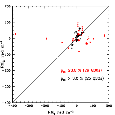
i) A comparison of the RM values from K08 and TSS09 reveals that the biggest differences in the RM datasets correspond to large RM values of K08 and sources having a low degree of polarization $p_{21}$. Here $p_{21}$ is the degree of polarization at   21 cm from TSS09 (average degree of polarization at the two wavelengths 20.89 cm $\&$ 21.96 cm). The situation is illustrated in Figure 1. Sources with $p_{21}>3.2\%$ (black cross, 25 QSOs) have quite similar RM values in both datasets and mostly crowd around the diagonal line. On the other hand sources with $p_{21}<3.2\%$ show a big scatter around the diagonal line. Furthermore there are sources which have large RM values ( $|\rm{RM}|>50$ rad m^-2) in the dataset of K08 but very low $|\rm{RM}|$ values in the sample of TSS09. The value of $p_{21}=3.2\%$ maximizes these effects in Figure 1.

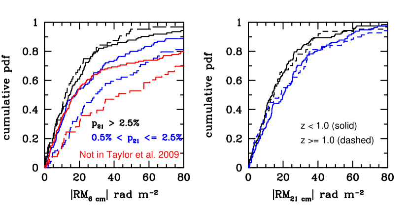
ii) Using a sample of 371 RM values from TSS09 at latitudes $|b|>30^{\circ}$ and for which the QSO’s redshifts, $z$, were available, we found no increase in the RM dispersion with $z$, contrary to the main finding of K08. The situation is illustrated in Figure 2, where the cumulative RM distributions at 6 cm (left panel) and 21 cm (right panel) are shown, split at the median fractional polarization of the total sample, $p_{21}=2.5\%$ (blue and black lines), and according to whether the source redshift is below or above $z=1.0$ (solid and dash line, respectively). The cumulative distribution of $|\rm{RM_{21}}|$ shows no evolution with $z$ in both low and high $p_{21}$ samples, whereas there is a significant broadening of the low $p_{21}$ ($0.5\%<p_{21}<2.5\%$) $|\rm{RM_{6}}|$ distribution with $z$. A Kolmogorov-Smirnov test (KS test) reveals that the RM distributions above and below $z=1.0$ are different at a significance level of 99.75%. We also show (red distributions) sources with determined $\rm{RM_{6}}$ values which are not in the Taylor et al. (2009) catalogue, but have declination $|\delta|>40^{\circ}$ and are thus in the NVSS. Most likely these sources are below the inclusion limits of the Taylor et al. (2009) catalogue, which are a $8\sigma$ detection in polarized intensity and $p_{21}>0.5\%$. A redshift evolution can be seen also for these sources with a similar significance level of 99.64%. Most likely the broadening of the RM distribution towards lower polarization $p_{21}$ is due to Galactic depolarization and possibly partly due to an increased error in RM, $\delta_{RM}$, towards lower polarized flux levels. This is supported by the fact that $\delta_{RM}\propto\delta_{P}/P$, where P is the polarized flux and $\delta_{P}$ its error (Brentjens & de Bruyn, 2005), and the high correlation between $p_{21}$ and polarized flux, as attested by a Kendall’s $\tau$ test, which yields $\tau=0.40$ and a chance probability of only $4.4\times 10^{-30}$ using all 371 RM values. However the broadening with z seen in the $|\rm{RM_{6}}|$ distributions is hard to explain by an observational bias. The interpretation of a $p_{21}$ dependent redshift evolution of the $|\rm{\rm{RM_{6}}}|$ distribution is however not straightforward either. In section 4 we show that it is crucial to distinguish between sight lines with/without intervening galaxies.

iii) The result of B08 that the RM distribution for QSOs with strong MgII systems along their sight lines is broader (at $\sim 95\%$ significance level) than for QSOs free of absorbers, completely disappears using the RM values of TSS09. Figure 3 shows the cumulative distribution (dash histograms) of $|\rm{RM_{21}}|$ values from TSS09 for sight lines with ($N_{\rm{MgII}}>0$, black)) and without MgII ($N_{\rm{MgII}}=0$, red) absorption systems. Clearly there is no difference between the two RM distributions. For comparison the solid histograms show the distributions of the $|\rm{RM_{6}}|$ values of B08.

2.3. Caveats

In the following sections we present a simple model to describe the impact of inhomogeneous, redshift dependent Faraday screens, on the polarization and RM of distant QSOs, as a function of wavelength.

However, additional effects may be at work when comparing quantities measured at different frequencies. In particular besides potential large uncertainties measured with both datasets, the low and high frequency emissions may originate from separate components in the source (e.g. the radio lobes and the compact core in a radio galaxy), inducing all sorts of frequency dependent effects, e.g., location, angular size, spectral indices and fractional polarization. For example, in some radio sources the fractional polarization appear to increase and then decrease with wavelength (Conway et al., 1974).

Also, while our model could be validated (or ruled out) by comparison of its predictions with observational data, this would require a high quality dataset, where the effects discussed above (and possibly others) are kept under strict control. Unfortunately such a dataset is not available to us at the moment, which forces us to refrain from such comparison. The latter, however, might be possible in the near future, with the delivery of new radio data from polarization surveys, either planned or just under way (see Sec. 5.2).

Figure 1.— Comparison of the RM values of K08 and TSS09, $\rm{RM_{6}}$ and $\rm{RM_{21}}$ respectively, splitted according to whether the degree of polarization is above (black crosses) or below (red filled circles) $p_{21}=3.2\%$. The two datasets differ especially for low $p_{21}$ values. Errors on $\rm{RM}_{6}$ are available for 24 of 54 RM measurments.

Figure 2.— Comparison of the cumulative distributions of RM values measured typically at 6cm (left panel) and at 21 cm (right panel). The samples are split according to the polarized fraction $p_{21}$ and the redshifts of the sources. Significant redshift evolution is seen in the $|\rm{RM_{6}}|$ values but not for the $|\rm{RM_{21}}|$ values. For sources with $0.5\%<p_{21}<2.5\%$ the RM distributions for sources above z=1 is broader than for sources below z=1, at a significance level of 99.75%. Red histograms are for NVSS sources not included in Taylor et al. (2009) catalogue. This is because they are below the inclusion limits of the catalogue, which are a 8$\sigma$ detection in polarized intensity and $p_{21}>0.5\%$. For these sources also a significant redshift evolution can be seen with a significance level of 99.64%.

Figure 3.— Comparison of the cumulative RM distributions of B08 (solid) and TSS09 (dash) for QSO sight lines with no MgII absorption systems (black lines) or with one or two, respectively (red lines). RM data in TSS09 were available for 54 out of the 71 QSOs in B08.

3. Depolarization by inhomogeneous Faraday screens

3.1. Previous work

In this section we develop a simple model to understand the effects arising from inhomogeneous Faraday screens and show that these can produce important depolarization effects that reproduce the differences of the RM datasets of K08 and TSS09.

The observed polarization $\mathbf{p}$ can be written as a complex number as:

$$\mathbf{p}=pe^{2i\chi},$$ (2)

where $p=P/I$ is the fractional degree of polarization given by the ratio of the polarized and total intensity, P and I, respectively and $\chi$ is the polarization angle determined by the other Stokes parameters, U and Q, as $\chi=1/2\arctan(U/Q)$.

The linear dependence between the polarization angle, $\chi$ and $\lambda^{2}$ stated in Eq. 1 is only valid for the case of a uniform foreground screen. Both the presence of unresolved inhomogeneities in the Faraday screen and/or sources of polarized radiation embedded within the Faraday active region produce increasing depolarization of the source at longer wavelength (Burn, 1966; Tribble, 1991; Sokoloff et al., 1998). This leads to nonlinear dependencies of the polarization angles and $\lambda^{2}$. In such cases detailed modeling is necessary for the correct interpretation of the RMs and for their use in measurements of magnetic fields.

There are several mechanisms that can reduce the fractional degree of polarization either in the radio source itself or in its foreground:

• Burn (1966); Sokoloff et al. (1998) showed that random fluctuations in the magnetic field within the source lead to a wavelength independent reduction of the degree of polarization. The latter is given by the ratio of the regular-to-total magnetic field energy, $p_{0}=p_{t}(\gamma)B_{r}^{2}/B^{2}$, where $p_{t}(\gamma)=\frac{3\gamma+3}{3\gamma+7}$ is the theoretical value of the degree of polarization which depends on the spectral index $\gamma$ of the emitting relativistic electrons ($\sim 0.74$ for $\gamma\sim 2.8$), and $p_{0}$ is the degree of polarization as $\lambda\to 0$.

• A further effect which reduces the degree of polarization is differential Faraday Rotation (Sokoloff et al., 1998). This effect happens if the synchrotron emission and the medium producing the Faraday rotation are not spatially separated. In such a case polarization angles from different depths within the source are rotated differently. The line of sight integrated emission suffers increasing depolarization with increasing wavelength. For extragalactic sources this effect seems not to be important (Tribble, 1991).

• Inhomogeneous Faraday Rotation screens within the radio beam lead to depolarization of the sources. If the RM screen is modelled by many independent RM cells, this effect is called depolarization by external Faraday dispersion (Burn, 1966; Sokoloff et al., 1998). If the RM screen varies systematically within the radio beam this effect is called beam depolarization.

Burn (1966) gives the formula

$$p=p_{0}\exp(-2\sigma_{RM}^{2}\lambda^{4})$$ (3)

to describe the depolarization induced by an inhomogeneous Faraday screen with a RM dispersion $\sigma_{RM}$. Assuming for simplicity that each RM cell is a cube of linear size $l_{0}$, then each cell contributes a dispersion $\sigma_{c}=0.81Bn_{e}l_{0}$ and $\sigma_{RM}=\sigma_{c}\sqrt{\eta}$, where $\eta=L/l_{0}$ is the number of cells along the path-length L traversed by the radio waves.

The size of the cell is determined by the scale above which the RM contributions are uncorrelated and can be determined by computing the structure function in high resolution RM maps.

Rossetti et al. (2008) and Mantovani et al. (2009) modelled polarisation observations of $\sim 65$ compact steep spectrum sources between 2.8 to 21 cm done with the WSRT, VLA and Effelsberg telescope. They observed that the fractional degree of polarisation at large wavelengths is too large to be explained by Burn’s depolarization law (Eq.3). They observed that for a large fraction of sources p remains approximately constant above 6 - 13 cm. To account for these observation they suggested that just a fraction of the polarised source is covered by a depolarising inhomogeneous RM screen and modified Eq. 3 to

$$p=p_{0}(f_{c}\exp(-2\sigma_{RM}^{2}\lambda^{4})+(1-f_{c})),$$ (4)

where $f_{c}$ is the covering factor of the source.

Here we emphasize that partial coverage of the polarized source by inhomogeneous RM screens is the key for explaining the differences in the RM values of K08 and TSS09.

4. Modelling

4.1. Extension to cosmological screens

In Eq. 4 the ($1+z)^{-2}$ correction for cosmological distances is not included. Assuming that the RM dispersion causing the depolarization, $\sigma_{RM}$, is constant with z, we modify Eq. 4 for cosmological sources as:

$$p=p_{0}(f_{c}\exp(-2\sigma_{RM}^{2}(1+z)^{-4}\lambda^{4})+(1-f_{c})).$$ (5)

Thus the width of $p(\lambda)$ changes as a function of z as

$$\sigma_{p}=\frac{(1+z)^{2}}{2\sigma_{RM}}.$$ (6)

This shows that depolarization by a non-evolving rest frame Faraday dispersion screen is expected to decrease for screens at higher redshift. Below, we explicitly compute the depolarization by typical RM screens as a function of redshift of the sources.

4.2. A simple model

In our model the Faraday screens consist of three components: (i) an inhomogeneous foreground screen local to the source with covering factor $f_{c,QSO}$, (ii) an inhomogeneous foreground screen in intervening galaxies with covering factors $f_{c,MgII}$ and (iii) a homogeneous screen due to the Milky Way, which is assumed uniform across the extension on the sky of the polarized source.

The uniform Faraday screen in the Milky Way is set to a constant value, $RM_{MW}=-10\>\rm{rad\>m^{2}}$. This value is consistent with Schnitzeler (2010) who determined the Milky Way contribution of Rotation Measures at $|b|>20^{\circ}$ using the Taylor et al. (2009) data.

On the other hand, each inhomogeneous foreground Faraday screen is characterized by an ensemble of cells of size $l_{0}$ with uncorrelated RM values. The RM values have a Gaussian distribution with dispersion $\sigma_{RM_{x}}/(1+z_{x})^{2}$ and zero mean, where $\sigma_{x}$ is the rest-frame RM dispersion, $z_{x}$ the screen’s redshift and, $x=QSO,MgII,$ labels different screens types, for which the above parameters may differ.

If the RM screen is at the source redshift and the source has linear size $s$, then it is covered by $N=s^{2}/l_{0}^{2}$ cells. Of these, only a fraction $f_{c,x}$ will be Faraday active for each screen. If the RM screen is at the redshift of the MgII systems, $s$ is the projected linear size of the source viewed from the Earth at the distance to the MgII system.

Each screen is then fully described by a realization of $N$ RM values, a fraction $f_{c,x}$ of which are extracted from the associated Gaussian distribution to characterize the active cells, while the reminder are set to zero to represent the inactive cells. Assuming a uniform flux of normalized intensity (I=1) and uniform (zero) intrinsic polarization angle across the source surface, we can write the following relations for the remaining non-zero Stokes parameter U, Q, the angle and degree of polarization, respectively,

$$U(\lambda^{2}) =\frac{1}{N}\sum_{i=1}^{N}\sin\left(2RM_{i}\lambda^{2}\right)$$ (7)

$$Q(\lambda^{2}) =\frac{1}{N}\sum_{i=1}^{N}\cos\left(2RM_{i}\lambda^{2}\right)$$ (8)

$$\chi(\lambda^{2}) =\frac{1}{2}\arctan\left(\frac{U}{Q}\right)$$ (9)

$$p(\lambda^{2}) =\sqrt{U^{2}+Q^{2}},$$ (10)

where

$$RM_{i}=RM_{QSO,i}+RM_{MgII,i}+RM_{MW},$$ (11)

are random variables determined by a Monte-Carlo realization.

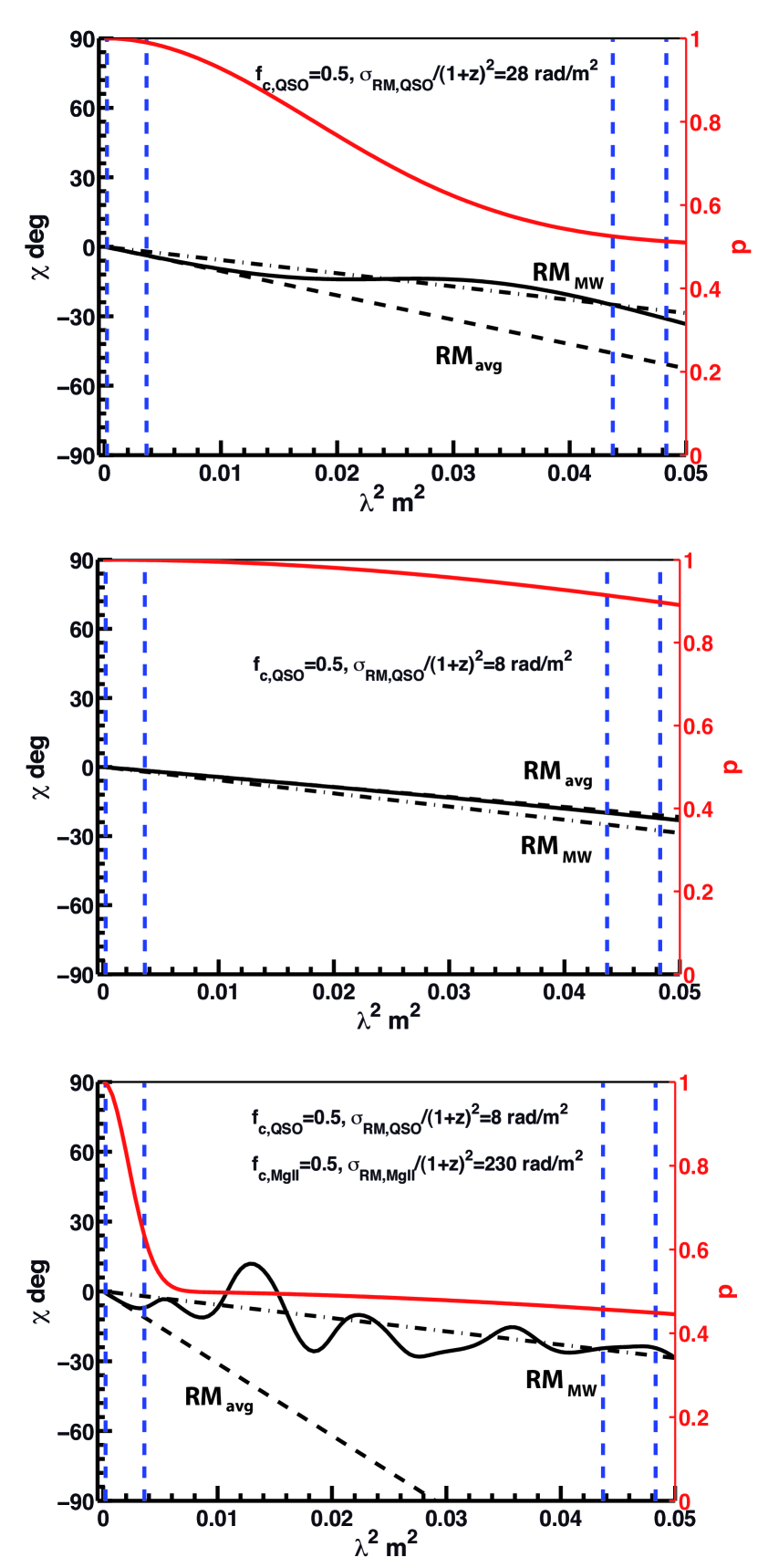
In Figure 4 we present generic results for three representative cases, namely a low ($z_{QSO}<1$) and high ($z_{QSO}>1$) redshift QSO with no intervening absorber in the top and mid panel, respectively, and a high redshift QSO with intervening absorber in the bottom panel. More detailes are specified below. In all cases, the inhomogeneous screen comprise eight cells, $N\,f_{c,x}=8$.

In each panel we plot the polarization angle, $\chi$ (black solid line – left y-axis), and the polarization fraction, p (red solid line – right y-axis) as a function of $\lambda^{2}$. To emphasize the importance of the effects of depolarization, we also show the rotation in polarization angle produced by (a) the average RM within the beam (dash line),

$$\chi=RM_{avg}\lambda^{2},$$

where

$$RM_{avg}= \frac{1}{N}\sum_{i=1}^{N}RM_{i}$$ (12)

$$= RM_{MW}+\frac{1}{N}\sum_{i=1}^{N}RM_{QSO,i}+RM_{MgII,i},$$ (13)

and (b) by the Milky Way (dash-dot line),

$$\chi=RM_{MW}\lambda^{2}.$$

Note that $RM_{avg}$ is in general non-zero and different from $RM_{MW}$. This is because for fixed fraction of active cells the second term in Eq. 13 is a random number of aplitude $1/\sqrt{N}$, with null probability of being either zero or $-RM_{MW}$. Finally, from left to right, the vertical blue dash lines indicate the typical observational wavelength of 20 GHz for (Jackson et al., 2010; Murphy et al., 2010), of 5 GHz for K08 and of 1.435 GHz and 1.365 GHz for the NVSS survey (Condon et al., 1998)) and Taylor et al. (2009).

The top panel illustrates the case of a low redshift sources ($z<1.0$), with observed RM dispersion of $\sigma_{RM,QSO}/(1+z)^{2}=28\;\rm{rad\>m^{-2}}$, $f_{c,QSO}=0.5$ and no intervening MgII absorber ($f_{c,MgII}=0$). It can be seen that at short wavelengths, $\lambda^{2}<0.014$, application of the simple $\lambda^{2}$ relation in Eq. 1, yields the average RM within the beam from which the RM distributions in the foreground screens can be inferred (Bernet et al., 2008). However, at longer wavelengths the flux through the inhomogeneous screen is depolarized so that the change in polarization angle is dominated by the contribution of the Milky Way. Correspondingly, the degree of polarization is given by $p\sim 1-f_{c,QSO}$.

The mid panel illustrates the case for a high redshift source, $z>1.0$ with observed RM dispersion of $\sigma_{RM,QSO}/(1+z)^{2}=8\;\rm{rad\>m^{-2}}$ and $f_{c,QSO}=0.5$. In this case, depolarization is negligible up to $\lambda^{2}=0.05$ or at 1.4 GHz. This means across most of the considered wavelength range application of the $\lambda^{2}$ relation in Eq. 1 would yield the average RM contributed by both the QSO screen and the Milky Way.

Finally, the bottom panel illustrates the same case as the mid panel but with an additional Faraday screen due to an absorber, with $\sigma_{RM,MgII}/(1+z)^{2}\sim\>230\>\rm{rad\>m^{-2}}$ and $f_{c,MgII}=0.5$.

This case has direct connection to the study of B08, who showed that intervening galaxies traced by MgII absorption lines contribute an additional Faraday screen with an observed rest frame RM dispersion $\sigma_{MgII}=140\;\rm{rad\;m^{-2}}$. In the context of our simple model, this implies a RM dispersion of the individual cells of the screen, responsible for the depolarization, $\sigma_{RM,MgII}=\sigma_{MgII}\sqrt{N/f_{c,MgII}}$. The value for $\sigma_{RM,MgII}/(1+z)^{2}$ assumed above is is based on this relation and the choice of $N\,f_{c,MgII}=8$. The bottom panel of Fig. 4 shows that with this choice of parameters the intervening screen causes significant depolarization above $\lambda^{2}\sim 0.003\rm{m^{2}}$. In this case the application of the $\lambda^{2}$ relation at longer wavelengths yields the Milky Way RM value.

The approach taken here, is valid in the limit of large number of random cells. Using the total flux - angular diameter relation given by Windhorst et al. (1984) we can estimate the extension of the region of the polarized emission. The median flux of our sources which are in the Taylor et al. (2009) catalogue (371 sources) is 1.2 Jy. This translates to a median source size in total flux of $\sim$ 10 arcsecs. Since the polarized emission is likely to be dominated by some hotspots the effective size in polarized emission is expected to be smaller than that. Given that the extension of the polarized emission is a few arcsecs and what we know about the scale of fluctuations of the RM (see next section) we expect a significant number of cells within the beam. In addition, using Eq. 5 and future multi-wavelength radio polarization observations one can determine $\sigma_{RM,MgII}$ and $f_{c,MgII}$ directly and thus calculate N.

Finally, we have assumed a homogeneous RM screen in the Milky Way. Gaensler et al. (2005), however, shows that arcsec scale fluctuation exist in the RM screen of the Large Magellanic Cloud and Haverkorn et al. (2008) shows that there are RM fluctuation in the local interstellar medium. Inhomogeneous Galactic RM contribution, which might vary for different sight lines, would lead to additional depolarization and add scatter to the predicted trends (see section 4.3) of our simple model, but cannot mimic them.

4.3. Model predictions

Based on this toy model with the free parameters $f_{c,x}$, $\sigma_{RM,x}$, we can predict simple trends in the observed angle and degree of polarization measured at fixed frequency as a function of radio source’s redshift. For simplicity we shall assume there is no redshift evolution in the model parameters. We must also distinguish between the two cases with and without the Faraday screen provided by intervening galaxies.

For the case without intervening galaxies the model predicts

• that towards low redshifts $p_{21}/p_{\lambda\rightarrow 0}\sim 1-f_{c,QSO}$, because the flux through the inhomogeneous Faraday screen is depolarized.

• that towards high redshift $p_{21}/p_{\lambda\rightarrow 0}\approx 1$ because the depolarization effects are suppressed. However, $p_{21}/p_{\lambda\rightarrow 0}$ anti-correlates with $\sigma_{RM,QSO}$ due to residual depolarization effects associated with the local screen.

• that towards low redshifts the discrepancy $|\rm{RM_{\lambda\rightarrow 0}-RM_{21}}|$ increases because due to depolarization effects $\rm{RM_{\lambda\rightarrow 0}}$ measures $\rm{RM_{avg}}$ while $\rm{RM_{21}}$ is dominated by the Milky Way contribution.

• that the discrepancy $|\rm{RM_{\lambda\rightarrow 0}-RM_{21}}|$ decreases towards high redshifts because both $\rm{RM_{\lambda\rightarrow 0}}$ and $\rm{RM_{21}}$ tend to measure the average $\rm{RM_{avg}}$ (Eq. 12).

For the case with intervening galaxies the model predicts

• that at all redshift the discrepancy $|\rm{RM_{\lambda\rightarrow 0}-RM_{21}}|$ is large, because due to depolarization effects $\rm{RM_{\lambda\rightarrow 0}}$ measures $\rm{RM_{avg}}$ and $\rm{RM_{21}}$ is dominated by the Milky Way contribution.

• that at all redshift $p_{21}/p_{\lambda\rightarrow 0}\lesssim 1-f_{c,MgII}$ because the sources will be significantly depolarized.

Figure 4.— Angle of polarization, $\chi$ (black solid line – left y-axis), and theoretical polarization fraction, p (red solid line – right y-axis), as a function of $\lambda^{2}$, for three models of inhomogeneous Faraday screens: a low (top) and high (mid) redshift QSO with no intervening absorbing system, and a high redshift QSO with intervening absorber (bottom). The dash line indicates the rotation of polarization angles due to the average RM within the beam, $\chi=RM_{avg}\lambda^{2}$, and the dash-dot line that due to the Milky Way, $\chi=RM_{MW}\lambda^{2}$. The vertical blue dash lines from left to right, indicate typical wavelength of observations at 1.5 cm, at 6 cm (K08), and at 20.89 cm and 21.96 cm (NVSS survey, Condon et al. (1998)) for Taylor et al. (2009) calculated RM values. In the top and mid panel the Faraday screens include an inhomogeneous screen local to the source with a covering factor $f_{c}=0.5$ and a screen in the Milky Way that is uniform across the source extension. In the top panel the source QSOs is at $z<1.0$ and has $\sigma_{RM,QSO}/(1+z)^{2}=28\;\rm{rad\>m^{-2}}$; in the mid panel the QSO is at $z>1.0$ and has $\sigma_{RM,QSO}/(1+z)^{2}=8\;\rm{rad\>m^{-2}}$. The bottom panel is the same as the mid panel with an additional Faraday screen due to an intervening system, with $\sigma_{RM,MgII}/(1+z)^{2}\sim\>230\>\rm{rad\>m^{-2}}$ and $f_{c}=0.5$.

5. Discussion

5.1. Nature of the partial inhomogeneous RM screen

It is instructive to look at high resolution Very Long Baseline Array (VLBA) radio polarization observations of some of our objects in K08. Examples of sources where VLBA polarization observations exist are 3C43 (Cotton et al., 2003), 3C118 (Mantovani et al., 2009) and B1524-026 (Mantovani et al., 2002). Typical resolutions of these observations are $\sim 8\times 8\>\rm{mas^{2}}$, which corresponds to a resolution of $64\>\rm{pc}\times 64\>\rm{pc}$ at $z\sim 1$. At such a high resolution complex structures in polarization angles and RM maps are revealed. Often it can be seen, e.g B1524-026 (Mantovani et al., 2002) that there is a dominant compact component in polarised flux and a more extended diffuse polarised component. Further it can be seen that the diffuse component consist of many independent RM cells. That means that for unresolved observations at large wavelengths the diffuse component will cancel and the more compact component dominates the observations.

For some sources it possible that the number of cells $f_{c}N$ in the RM screen is very low. In this case no depolarization is observed but p and $\chi$ oscillate. This situation was observed for the source 3C 27 by Goldstein & Reed (1984). Rossetti et al. (2008) fitted a two component model to the data to describe p and $\chi$ for the source B3 0110+401. Farnsworth et al. (2011) also used a two component model to describe radio polarization observation at large wavelengths $\lambda\sim 1$ m.

For the sightlines with intervening galaxies it is very natural to assume that the magnetic fields within them will lead to depolarization, an effect studied in the LMC by Gaensler et al. (2005). Using the Milky Way as typical galaxy we would expect depolarization of the background QSOs. For NGC 1310 this effect was observed by Fomalont et al. (1989) and Schulman & Fomalont (1992). One possibility is that the source covers both the spiral arms and interarm regions. For the spiral arms the coherence lengths of the magnetic fields are much shorter as suggested by observations of Haverkorn et al. (2008). These authors gives an outer scale of turbulence of 0.1 kpc for interarm regions and 10 pc for the spiral arms in the Milky Way. In this way the area covered by the spiral arms would be depolarized and the interarms would produce a coherent screen. Other interpretations are again as for the QSO itself that the polarized emission is dominated by one compact component which competes with a more extended diffuse emission. If the size of the compact component is small enough, this component could get a coherent screen whereas the extended source gets different RM screens which will lead to depolarization of this component.

5.2. Rotation Measure Synthesis

At the moment there are several polarization surveys under way or planned, e.g. GALFACTS (Taylor & Salter, 2010), LOFAR (Anderson et al., 2012), or POSSUM (Gaensler et al., 2010) within ASKAP. These polarization surveys should pave the way for the planned polarization survey for SKA (Gaensler et al., 2004; Gaensler, 2009; Beck & Gaensler, 2004). In particular one wishes to study the evolution of magnetic fields in galaxies and in the intergalactic medium as a function of cosmic time using large RM datasets.

Figure 5.— Original Faraday spectrum for a low redshift QSO and its associated observed polarization angle and degree, together with the recovered Faraday spectrum for a finite wavelength coverage. The Monte Carlo realization is identical to the top panel in Figure 4. Upper left panel: Original Faraday spectrum for a low redshift QSO with a homogeneous Milky Way RM screen of $\rm{RM}=-10\>\rm{rad\>m^{2}}$ and an inhomogeneous intrinsic RM screen with $\sigma_{RM,QSO}/(1+z)^{2}=28\>\rm{rad\>m^{-2}}$ and a covering factor $f_{c}=0.5$. Upper middle panel: Corresponding U and Q Stokes parameters (thin solid line, thin dashed line) and degree of polarization p (thick solid line) as a function of $\lambda^{2}$. An observational error $\sigma_{U,Q}\approx 0.017\%$ is added to every channel. Upper right panel: Corresponding polarization angle $\chi$ vs. $\lambda^{2}$. The dashed line indicates the expected polarization angle from the homogeneous Milky Way RM contribution. Lower left panel: Recovered Faraday spectrum for the wavelength range $\lambda_{min}=0.03\rm{m}$ to $\lambda_{max}=0.27\rm{m}$. The thin solid/dashed line indicates the real/imaginary part of the spectrum and the thick solid line shows the amplitude. Lower middle panel: Faraday spectrum after applying the CS-RM-Thin method of Li et al. (2011) to correct for the limited wavelength coverage.

Figure 6.— Identical to Figure 5 but for the case of a high redshift QSO with an intervening MgII system. The Monte Carlo realization is identical to the bottom panel in Figure 4

Figure 7.— Identical to Figure 6 with same $\Delta\lambda^{2}$ coverage and thus identical Faraday depth resolution $\delta\phi$ but with observations done at longer wavelengths.

With the large number of available spectral channels in these surveys, e.g. a few thousands, Faraday Rotation Measure Synthesis (Brentjens & de Bruyn, 2005) can be performed. Using this technique one performs a Fourier transformation of the observed complex polarization $p(\lambda^{2})$ to obtain a Faraday depth spectrum $F(\phi)$. Here the case of a single uniform Faraday screen corresponds to a delta function in Faraday depth space and in this case the Faraday depth is equal to the traditional RM (Eq. 1).

Basic parameters for a Faraday survey are the maximum observable Faraday depth, $\phi_{max}\approx\sqrt{3}/\delta\lambda^{2}$, the Faraday depth resolution, $\delta\phi\approx 2\sqrt{3}/\Delta\lambda^{2}$ and the largest scale in Faraday depth that one is sensitive to, max-scale $\approx\pi/\lambda_{min}^{2}$. Here $\delta\lambda^{2}$ is the channel width, $\Delta\lambda^{2}$ is the total bandwidth and $\lambda_{min}^{2}$ is the smallest wavelength (squared) of the observations. Regions which produce only Faraday rotation but do not emit polarized radiation can be described by Dirac $\delta$ functions in $\phi$ space and are Faraday-thin sources (Brentjens & de Bruyn, 2005). Below we discuss our model of the depolarization of QSOs in terms of Faraday Rotation Measure Synthesis. This is to provide some basic comparisons for ongoing or future RM surveys. See e.g. O’Sullivan et al. (2012) for current observations of Faraday depth spectra.

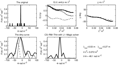
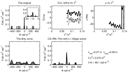
In the next, with the auxilium of Fig. (5)–(7) we give a simple example of the application of RM-synthesis to the same cases studied in Figure 4, which illustrates the advantages of this emerging technique. In Figure 5 the original Faraday spectrum for a low redshift QSO without intervening galaxies is shown. Here the Monte Carlo realization is the same as in Figure 4 (upper panel) with adopted parameters $\sigma_{RM,QSO}/(1+z)^{-2}=28\>\rm{rad\>m^{-2}}$ and $f_{c,QSO}=0.5$. In particular, all of the 16 cells have the contribution from the MW and eight cells have an additional intrinsic low-z QSO contribution. The Faraday spectrum is only real valued which means that the intrinsic polarization angles are zero. The adopted minimum and maximum wavelengths are $\lambda_{min}=0.03\>\rm{m}$ and $\lambda_{max}=0.27\;\rm{m}$ and correspond to a Faraday depth resolution of $\delta\phi\approx\>48.1\>\rm{rad\>m^{-2}}$. The choosen wavelength range corresponds to the offered wavelength range at the Australia Telescope Compact Array which is similar to the EVLA (Beck et al., 2012). The recovered Faraday spectrum with this resolution is shown in the lower left panel.

There are several methods to recover the information lost due to the incomplete wavelength coverage (Heald et al., 2009; Li et al., 2011). We use here the compressive sampling (CS) method of Li et al. (2011). Best results are obtained if prior information about the Faraday spectrum is present, e.g. if the sources are Faraday thin or thick. The obtained Faraday spectrum after applying the CS RM thin method of Li et al. (2011) to the Q and U vectors (upper middle panel) is shown in the lower right panel. It can be seen that the homogeneous RM component at -10 $\rm{rad\>m}^{-2}$ can be approximately recovered, but not all of the inhomogeneous RM components.

In Figure 6 the Faraday spectrum for a high redshift QSO with an intervening galaxy is shown. Here the Faraday spectrum is identical to the one used in Figure 5 in the lower panel with the parameters $\sigma_{RM,MgII}/(1+z)^{2}\sim\>230\>\rm{rad\>m^{-2}}$ and $f_{c,MgII}=0.5$, $\sigma_{RM,QSO}/(1+z)^{2}\sim\>8\>\rm{rad\>m^{-2}}$ and $f_{c,QSO}=0.5$, and $\rm{RM}=-10\>\rm{rad}\>m^{-2}$. In the Monte Carlo realization shown in Figure 6 all of the 16 cells have the contribution from the MW, eight (random) cells have an additional intrinsic high-z QSO contribution and eight (random) cells have an additional contribution from the intervening galaxy. With the observational parameters $\lambda_{min}=0.03\>\rm{m}$ and $\lambda_{max}=0.27\>\rm{m}$ and $\delta\phi\approx 48.1\;\rm{rad\>m^{-2}}$ the MW+QSO components can not be resolved but lead to a distinct peak at $\phi\approx-10\;\rm{rad}\;\rm{m}^{-2}$ with an amplitude $\sim 0.45$ $\rm{m}^{2}\>\rm{rad^{-1}}$ in the recovered Faraday spectrum. On the other hand, the eight RM components with contributions from intervening galaxies can be well resolved with the assumed covered wavelength range.

For comparison in Figure 7 we show the recovered Faraday spectrum for observations using longer wavelengths, $\lambda_{min}=0.27\>\rm{m}$ and $\lambda_{max}=0.38\>\rm{m}$ but with the same covered wavelength range $\Delta\lambda^{2}$. This shows that the qualitative features of the Faraday spectrum are also recovered, although with a lower quality than in Fig. 6.

In summary, from section 4.3 using polarization angle $\chi$ vs. $\lambda^{2}$ observations one might conclude that it is best to do observations at short wavelengths (below the exponential fall off) in order to measure the average RM. However as we have illustrated above using RM Synthesis this is not necessary. In order to be able to resolve the individual RM components a large $\Delta\lambda^{2}$ is required. (See Beck et al. (2012) for a summary of the Faraday depth resolution $\delta\phi$ of current and future radio telescopes.) The proposed wavelength range for SKA with $\lambda\sim 0.03-4.3\>\rm{m}$ and $\Delta\lambda\sim 18\>\rm{m^{2}}$ and $\delta\phi\sim\>0.2\>\rm{rad}\>\rm{m}^{-2}$ will offer a superb Faraday resolution to resolve individual RM components in intervening galaxies.

6. Summary and conclusions

In previous work we have used RM values from K08, typically determined at 6 cm, to study magnetic fields in normal galaxies at high redshift. When the analysis was repeated using the recently released RM data of TSS09, determined at 21 cm, we could find neither a correlation between $|$RM$|$ and absorbing systems as in B08, nor an increase in the RM dispersion with z as found in K08. Motivated by the above results, we have attempted to understand those differences in terms of a simple model based on inhomogeneous Faraday screens associated both with the QSO and the MgII host galaxies, and for both low and high redshift.

We find that the presence of inhomogeneous screens leads to important departures from the classical $\lambda^{2}$ dependence of the rotation of the polarization angle. Related to this are depolarization effects which become stronger towards higher wavelengths. As a result, due to cosmological redshift, observations at fixed wavelength are affected differently by depolarization and are sensitive to different Faraday active components. In particular depolarization effects become stronger for lower redshift QSOs. We find that the depolarization saturates to a value given by the intrinsic polarization times the complement of the covering factor of the inhomogeneous screen, $(1-f_{c})$.

Actual predictions depend on the assumed values for the model parameters. The following results apply for the choices made in section. 4, which are relevant for the current investigation. When the line of sight to the QSO is free of absorption systems, application of the $\lambda^{2}$ analysis to extract RM values from radio observations then has the following consequences:

• for low redshift QSOs, $\rm{RM_{21}}$ is dominated by the Milky Way contribution, while $\rm{RM_{\lambda\rightarrow 0}}$ measures $\rm{RM_{avg}}$ (see Eq. 12).

• for high redshift QSOs, in general the RM value reflect $\rm{RM_{avg}}$

The presence of absorption systems contributes an additional Faraday screen which further depolarizes the low frequency radiation. Therefore,

• while $\rm{RM_{\lambda\rightarrow 0}}$ is given by $\rm{RM_{avg}}$, $\rm{RM_{21}}$ is dominated by the Milky Way contribution and the discrepancy $|\rm{RM_{\lambda\rightarrow 0}-RM_{21}}|$ is large at all redshifts.

In conclusion, while the model is admittedly simple, it seems plausible to consider that the discrepancy between results based on K08 and TSS08 RM are due to the severe depolarization induced by inhomogeneous Faraday screen on high wavelength radiation. This, however, does not exclude the importance of other effects.

Finally, the study of magnetic fields in galaxies as a function of cosmic time will benefit considerably from the application of RM-synthesis, which has the power to disintangle the contribution from inhomogeneous magneto-active components. For this purpose, instrumental bandwidth is most important, although higher frequency channels appear to deliver higher quality. This conclusions may be refined with future investigations.

References

- Anderson et al. (2012) Anderson, J., Beck, R., Bell, M., et al. 2012, arXiv:1203.2467
- Arshakian & Beck (2011) Arshakian, T. G., & Beck, R. 2011, MNRAS, 418, 2336
- Beck et al. (2012) Beck, R., Frick, P., Stepanov, R., & Sokoloff, D. 2012, A&A, 543, A113
- Beck & Gaensler (2004) Beck, R., & Gaensler, B. M. 2004, NewAR, 48, 1289
- Bernet et al. (2008) Bernet, M. L., Miniati, F., Lilly, S. J., Kronberg, P. P., & Dessauges-Zavadsky, M. 2008, Nature, 454, 302
- Bernet et al. (2010) Bernet, M. L., Miniati, F., & Lilly, S. J. 2010, ApJ, 711, 380
- Brentjens & de Bruyn (2005) Brentjens, M. A., & de Bruyn, A. G. 2005, A&A, 441, 1217
- Burn (1966) Burn, B. J. 1966, MNRAS, 133, 67
- Condon et al. (1998) Condon, J. J., Cotton, W. D., Greisen, E. W., Yin, Q. F., Perley, R. A., Taylor, G. B., & Broderick, J. J. 1998, AJ, 115, 1693
- Conway et al. (1974) Conway, R. G., Haves, P., Kronberg, P. P., et al. 1974, MNRAS, 168, 137
- Cotton et al. (2003) Cotton, W. D., Spencer, R. E., Saikia, D. J., & Garrington, S. 2003, A&A, 403, 537
- Farnsworth et al. (2011) Farnsworth, D., Rudnick, L., & Brown, S. 2011, AJ, 141, 191
- Fomalont et al. (1989) Fomalont, E. B., Ebneter, K. A., van Breugel, W. J. M., & Ekers, R. D. 1989, ApJ, 346, L17
- Gaensler et al. (2005) Gaensler, B. M., Haverkorn, M., Staveley-Smith, L., et al. 2005, Science, 307, 1610
- Gaensler (2009) Gaensler, B. M. 2009, IAU Symposium, 259, 645
- Gaensler et al. (2004) Gaensler, B. M., Beck, R., & Feretti, L. 2004, AN, 48, 1003
- Gaensler et al. (2010) Gaensler, B. M., Landecker, T. L., Taylor, A. R., & POSSUM Collaboration 2010, Bulletin of the American Astronomical Society, 42, #470.13
- Goldstein & Reed (1984) Goldstein, S. J., Jr., & Reed, J. A. 1984, ApJ, 283, 540
- Hammond et al. (2012) Hammond, A. M., Robishaw, T., & Gaensler, B. M. 2012, arXiv:1209.1438
- Haverkorn et al. (2008) Haverkorn, M., Brown, J. C., Gaensler, B. M., & McClure-Griffiths, N. M. 2008, ApJ, 680, 362
- Heald et al. (2009) Heald, G., Braun, R., & Edmonds, R. 2009, A&A, 503, 409
- Jackson et al. (2010) Jackson, N., Browne, I. W. A., Battye, R. A., Gabuzda, D., & Taylor, A. C. 2010, MNRAS, 401, 1388
- Kronberg et al. (2008) Kronberg, P. P., Bernet, M. L., Miniati, F., Lilly, S. J., Short, M. B., & Higdon, D. M. 2008, ApJ, 676, 70
- Kronberg et al. (2012) Kronberg et al., in preparation
- Li et al. (2011) Li, F., Brown, S., Cornwell, T. J., & de Hoog, F. 2011, A&A, 531, A126
- Mantovani et al. (2002) Mantovani, F., Junor, W., Ricci, R., Saikia, D. J., Salter, C., & Bondi, M. 2002, A&A, 389, 58
- Mantovani et al. (2009) Mantovani, F., Mack, K.-H., Montenegro-Montes, F. M., Rossetti, A., & Kraus, A. 2009, A&A, 502, 61
- Murphy et al. (2010) Murphy, T., et al. 2010, MNRAS, 402, 2403
- O’Sullivan et al. (2012) O’Sullivan, S. P., Brown, S., Robishaw, T., et al. 2012, MNRAS, 2504
- Rossetti et al. (2008) Rossetti, A., Dallacasa, D., Fanti, C., Fanti, R., & Mack, K.-H. 2008, A&A, 487, 865
- Schnitzeler (2010) Schnitzeler, D. H. F. M. 2010, MNRAS, 409, L99
- Schulman & Fomalont (1992) Schulman, E., & Fomalont, E. B. 1992, AJ, 103, 1138
- Simard-Normandin et al. (1981) Simard-Normandin, M., Kronberg, P. P., & Button, S. 1981, ApJS, 45, 97
- Sokoloff et al. (1998) Sokoloff, D. D., Bykov, A. A., Shukurov, A., et al. 1998, MNRAS, 299, 189
- Taylor et al. (2009) Taylor, A. R., Stil, J. M., & Sunstrum, C. 2009, ApJ, 702, 1230
- Taylor & Salter (2010) Taylor, A. R., & Salter, C. J. 2010, Astronomical Society of the Pacific Conference Series, 438, 402
- Tribble (1991) Tribble, P. C. 1991, MNRAS, 250, 726
- Windhorst et al. (1984) Windhorst, R. A., van Heerde, G. M., & Katgert, P. 1984, A&AS, 58, 1