Weakly nonlinear stability analysis of MHD channel flow
using an efficient numerical approach

?abstractname?

We analyze weakly nonlinear stability of a flow of viscous conducting liquid driven by pressure gradient in the channel between two parallel walls subject to a transverse magnetic field. Using a non-standard numerical approach, we compute the linear growth rate correction and the first Landau coefficient, which in a sufficiently strong magnetic field vary with the Hartmann number as $\mu_{1}\sim(0.814-\mathrm{i}19.8)\times 10^{-3}\textit{Ha}$ and $\mu_{2}\sim(2.73-\mathrm{i}1.50)\times 10^{-5}\textit{Ha}^{-4}.$ These coefficients describe a subcritical transverse velocity perturbation with the equilibrium amplitude $|A|^{2}=\Re[\mu_{1}]/\Re[\mu_{2}](\textit{Re}_{c}-\textit{Re})\sim 29.8\textit{Ha}^{5}(\textit{Re}_{c}-\textit{Re}),$ which exists at Reynolds numbers below the linear stability threshold $\textit{Re}_{c}\sim 4.83\times 10^{4}\textit{Ha}.$ We find that the flow remains subcritically unstable regardless of the magnetic field strength. Our method for computing Landau coefficients differs from the standard one by the application of the solvability condition to the discretized rather than continuous problem. This allows us to bypass both the solution of the adjoint problem and the subsequent evaluation of the integrals defining the inner products, which results in a significant simplification of the method.

I Introduction

A number of fluid flows can become turbulent while being linearly stable. Some of these flows, such as, for example, plane Couette flow and circular pipe (Hagen-Poiseuille) flow, are linearly stable at all velocities, while other may become linearly unstable at higher velocities. Typical examples of the latter class of flows are plane Poiseuille flow and its magnetohydrodynamic counterpart, Hartmann flow, which arises when a conducting liquid flows in the presence of a transverse magnetic field. Theoretically, the former is known to be linearly stable up to the critical Reynolds number $\textit{Re}_{c}=5722.22,$ (Orszag, 1971) however, experimentally it has been observed to become turbulent at Reynolds numbers as low as $10^{3}.$ (Carlson, Widnall & Peeters, 1982; Nishioka & Asai, 1985; Alavyoon, Henningson, & Alfredsson, 1986) Similarly, Hartmann flow becomes linearly unstable at the local critical Reynolds number based on the Hartmann layer thickness $R{}_{c}\approx 50\,000,$(Lock, 1955; Takashima, 1996) whereas turbulence in this flow can be observed at Reynolds numbers as low as $R_{t}\approx 400.$(Moresco & Alboussière, 2004; Krasnov et al., 2004, 2013)

Such a subcritical instability can be accounted for by positive feedback of the perturbation amplitude on its growth rate, which is a non-linear effect. Thus, a perturbation with sufficiently large amplitude can acquire positive growth rate at subcritical Reynolds numbers, where all small-amplitude perturbations are linearly stable. For small-amplitude perturbations in the vicinity of linear stability threshold this effect is described by the so-called Landau (Stuart-Landau) equation(Landau, 1944; Landau & Lifshitz, 1987). Whether an instability is sub- or supercritical is determined by the coefficients of this equation, which are referred to as Landau coefficients and have to be determined for each particular case.

It was first suggested by Lock (1955) that the instability of Hartmann flow may be due to finite-amplitude disturbances. This conjecture was supported by weakly nonlinear stability analysis of a physically similar asymptotic suction boundary layer.(Hocking, 1975; Likhachev, 1976) Later the same was found to be the case also for the Hartmann boundary layer.(Moresco & Alboussière, 2003)

Alternative explanations for the transition to turbulence in Hartmann flow are based on the energy stability and transient growth theories. Although the former applies to arbitrary disturbance amplitudes, it is essentially an amplitude-independent and, thus, linear approach. Namely, the nonlinear term drops out of the disturbance energy balance because it neither produces nor dissipates the energy. Using this approach Lingwood & Alboussière (1999) found the Hartmann layer to be energetically stable when $R_{e}\lesssim 26$, which ensures monotonic decay of all disturbances. This threshold is almost by an order of magnitude lower than that observed experimentally. As demonstrated in the numerical study by Krasnov et al., 2004the optimal transient growth mechanism, which has been studied for both the Hartmann boundary layer(Gerard-Varet, 2002) and for the whole Hartmann flow(Airiau & Castets, 2004), is also linear. As pointed out by Waleffe (1995), transition to turbulence is mediated by nonlinear unstable equilibrium states which are not directly related to the non-normality of the linearized problem responsible for the transient growth.

The basic formalism of weakly nonlinear stability analysis of plane Poiseuille flow by the method of amplitude expansion was introduced by Stuart (1960) and Watson (1960) and later modified by Reynolds & Potter (1967). Higher-order Landau coefficients for plane Poiseuille flow driven by a fixed pressure gradient were computed by Sen & Venkateswarlu (1983) using both aforementioned methods, which were found to perform comparably well at supercritical Re but not in the subcritical range, where Watson’s method encounters singularities. Asymptotic expansion methods for weakly nonlinear stability analysis have been reconsidered and surveyed by Herbert (1983), and substantially extended by Stewartson & Stuart (1971) who used the method of multiple scales to include slow spatial variation, which resulted in the complex Ginzburg-Landau equation.(Aranson & Kramer, 2002) The method of multiple scales was shown to be equivalent to that of amplitude expansion (Fujimura, 1989) as well as to that the center manifold reduction, which is another technique for deriving the Landau equation.(Fujimura, 1991)

The evaluation of Landau coefficients required in weakly nonlinear stability analysis is technically complicated by the necessity to solve the adjoint problem and the subsequent evaluation of complex inner product integrals containing the adjoint eigenfunction. In this paper, we employ a non-standard approach which is significantly simpler than the commonly used one.(Huerre & Rossi, 1998; Schmid & Henningson, 2001; Yaglom, 2012) Our method is based on the application of the solvability condition to the discretized rather than continuous problem. This allows us to evaluate Landau coefficients without using the adjoint eigenfunction, which in our approach is replaced by the left eigenvector. Such a possibility has been briefly discussed by Crouch & Herbert (1993) and a similar approach based on Gaussian elimination has been noticed also by Sen & Venkateswarlu (1983).

The paper is organized as follows. In the section to follow, we formulate the problem and consider general 2D traveling-wave solution, which is then expanded in small perturbation amplitude to obtain usual expressions for Landau coefficients. Section III presents a detailed development of our approach for Chebyshev collocation method. The method is validated in Sec. IV by computing Landau coefficients for plane Poiseuille flow driven either by fixed pressure gradient or flow rate. Section V presents numerical results concerning both linear and weakly nonlinear stability of Hartmann flow. The paper is concluded by a summary of results in Sec. VI.

II Formulation of problem

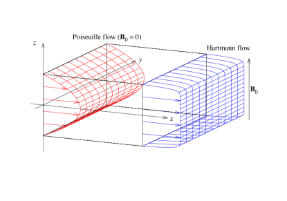
?figurename? 1: Sketch of the problem showing velocity profiles of Poiseuille and Hartmann flows.

Consider a flow of incompressible viscous electrically conducting liquid with the density $\rho,$ kinematic viscosity $\nu$ and electrical conductivity $\sigma$ driven by a constant gradient of pressure $p$ in the channel of the width $2h$ between two parallel walls in the presence of a transverse homogeneous magnetic field $\boldsymbol{\mathit{B}}$. The velocity distribution of the flow, $\boldsymbol{\mathit{v}}$, is governed by the Navier-Stokes equation

$$\partial_{t}\boldsymbol{\mathit{v}}+(\boldsymbol{\mathit{v}}\cdot\boldsymbol{\mathit{\nabla}})\boldsymbol{\mathit{v}}=-\rho^{-1}\boldsymbol{\mathit{\nabla}}p+\nu\boldsymbol{\mathit{\nabla}}^{2}\boldsymbol{\mathit{v}}+\rho^{-1}\boldsymbol{\mathit{f}},$$ (1)

where $\boldsymbol{\mathit{f}}=\boldsymbol{\mathit{j}}\times\boldsymbol{\mathit{B}}$ is the electromagnetic body force containing the induced electric current $\boldsymbol{\mathit{j}},$ which in turn is governed by Ohm’s law for a moving medium

$$\boldsymbol{\mathit{j}}=\sigma(\boldsymbol{\mathit{E}}+\boldsymbol{\mathit{v}}\times\boldsymbol{\mathit{B}}),$$ (2)

where $\boldsymbol{\mathit{E}}$ is the electric field in the stationary frame of reference. The flow is assumed to be sufficiently slow so that the induced magnetic field is negligible relative to the imposed one. This supposes a small magnetic Reynolds number $\textit{Re}_{m}=\mu_{0}\sigma v_{0}h\ll 1,$ where $\mu_{0}$ is the permeability of vacuum and $v_{0}$ is the characteristic velocity of the flow. In addition, we assume that the characteristic time of velocity variation is much longer than the magnetic diffusion time $\tau_{m}=\mu_{0}\sigma h^{2}.$ This allows us to use the quasi-stationary approximation leading to $\boldsymbol{\mathit{E}}=-\boldsymbol{\mathit{\nabla}}\phi,$ where $\phi$ is the electrostatic potential.(Roberts, 1967) The velocity and current satisfy mass and charge conservation $\boldsymbol{\mathit{\nabla}}\cdot\boldsymbol{\mathit{v}}=\boldsymbol{\mathit{\nabla}}\cdot\boldsymbol{\mathit{j}}=0.$ Applying the latter to Ohm’s law (2) yields

$$\boldsymbol{\mathit{\nabla}}^{2}\phi=\boldsymbol{\mathit{B}}\cdot\boldsymbol{\mathit{\omega}},$$ (3)

where $\boldsymbol{\mathit{\omega}}=\boldsymbol{\mathit{\nabla}}\times\boldsymbol{\mathit{v}}$ is vorticity. At the channel walls $S$, the normal $(n)$ and tangential $(\tau)$ velocity components satisfy impermeability and no-slip boundary conditions $\left.v_{n}\right|_{s}=0$ and $\left.v_{\tau}\right|_{s}=0.$ Electrical conductivity of the walls is irrelevant for the type of flow considered in this study.

We employ right-handed Cartesian coordinates with the origin set at the mid-height of the channel, the $x$- and the $z$-axes directed, respectively, against the applied pressure gradient $\boldsymbol{\mathit{\nabla}}p_{0}=P\boldsymbol{\mathit{e}}_{x}$ and along the magnetic field $\boldsymbol{\mathit{B}}=B\boldsymbol{\mathit{e}}_{z}$ so that the channel walls are located at $z=\pm h,$ as shown in figure 1, and the velocity is defined as $\boldsymbol{\mathit{v}}=(u,v,w).$ Subsequently, all variables are non-dimensionalized by using $h,$ $h^{2}/\nu$ and $h\nu B$ as the length, time and electric potential scales, respectively. The velocity is scaled by the viscous diffusion speed $\nu/h,$ which we employ as the characteristic velocity instead of the commonly used center-line velocity.

The problem admits a rectilinear base flow

$$\boldsymbol{\mathit{v}}_{0}(z)=\bar{u}_{0}(z)\boldsymbol{\mathit{e}}_{x}=\textit{Re}\,\bar{u}(z)\boldsymbol{\mathit{e}}_{x}$$ (4)

for which Eq. (1) reduces to

$$\bar{u}^{\prime\prime}-\textit{Ha}^{2}\bar{u}=\bar{P},$$ (5)

where $\textit{Re}=Uh/\nu$ is the Reynolds number based on the center-line velocity $U,$ $\textit{Ha}=hB\sqrt{\sigma/\rho\nu}$ is the Hartmann number, and $\bar{P}$ is a dimensionless pressure gradient satisfying the normalization condition $\bar{u}(0)=1.$ This equation defines the well-known Hartmann flow profile

$$\bar{u}(z)=\frac{\cosh(\textit{Ha})-\cosh(z\textit{Ha})}{\cosh(\textit{Ha})-1}$$ (6)

with $\bar{P}=-\frac{\textit{Ha}^{2}\cosh(\textit{Ha})}{\cosh(\textit{Ha})-1},$ which relates the center-line velocity with the applied pressure gradient $P=\bar{P}U\nu\rho/h^{2}.$ In the weak magnetic field $(\textit{Ha}\ll 1),$ the Hartman flow reduces to the classic plane Poiseuille flow $\bar{u}(z)=1-z^{2}.$

At sufficiently high $\textit{Re},$ the base flow can become unstable with respect to infinitesimal perturbations $\boldsymbol{\mathit{v}}_{1},$ which due to the invariance of the base flow in both $t$ and $\boldsymbol{\mathit{x}}=(x,y)$ can be sought as

$$\boldsymbol{\mathit{v}}_{1}(\boldsymbol{\mathit{r}},t)=\boldsymbol{\mathit{\hat{v}}}(z)\mathrm{e}^{\lambda t+\mathrm{i}\boldsymbol{\mathit{k}}\cdot\boldsymbol{\mathit{x}}}+\mbox{c.c.},$$ (7)

where $\boldsymbol{\mathit{\hat{v}}}(z)$ is complex amplitude distribution, $\lambda$ is temporal growth rate, and $\boldsymbol{\mathit{k}}=(\alpha,\beta)$ is the wave vector. The incompressibility constraint, which takes the form $\boldsymbol{\mathit{D}}_{1}\cdot\boldsymbol{\mathit{\hat{v}}}=0,$ where $\boldsymbol{\mathit{D}}_{1}\equiv\boldsymbol{\mathit{e}}_{z}\frac{\mathrm{d}\,}{\mathrm{d}z}+\mathrm{i}\boldsymbol{\mathit{k}}$ is a spectral counterpart of the nabla operator, is satisfied by expressing the component of velocity perturbation in the direction of the wave vector as $\hat{u}_{\shortparallel}=\boldsymbol{\mathit{e}}_{\shortparallel}\cdot\boldsymbol{\mathit{\hat{v}}}=\mathrm{i}k^{-1}\hat{w}^{\prime},$ where $\boldsymbol{\mathit{e}}_{\shortparallel}=\boldsymbol{\mathit{k}}/k$ and $k=|\boldsymbol{\mathit{k}}|.$ Taking the curl of the linearized counterpart of Eq. (1) to eliminate the pressure gradient and then projecting it onto $\boldsymbol{\mathit{e}}_{z}\times\boldsymbol{\mathit{e}}_{\shortparallel},$ after some transformations we obtain the Orr-Sommerfeld equation

$$\lambda\boldsymbol{\mathit{D}}_{1}^{2}\hat{w}=\left[\boldsymbol{\mathit{D}}_{1}^{4}-\textit{Ha}^{2}(\boldsymbol{\mathit{e}}_{z}\cdot\boldsymbol{\mathit{D}}_{1})^{2}+\mathrm{i}k\textit{Re}(\bar{u}^{\prime\prime}-\bar{u}\boldsymbol{\mathit{D}}_{1}^{2})\right]\hat{w},$$ (8)

which contains the electromagnetic term proportional to $\textit{Ha}^{2}.$ The no-slip and impermeability boundary conditions require

$$\hat{w}=\hat{w}^{\prime}=0\quad\mbox{at}\quad z=\pm 1.$$ (9)

The equation above is written in a non-standard form corresponding to our choice of the characteristic velocity. Note that Reynolds number appears in this equation as a factor at the convective term rather than its reciprocal at the viscous term as in the standard form. As a result, the growth rate $\lambda$ differs by a factor of Re from its standard definition. In this form, the equation is slightly more convenient for the subsequent numerical solution.

Since the equation above admits Squire’s transformation as in the non-magnetic case,(Drazin & Reid, 1981) in the following we consider only two-dimensional perturbations $(k=\alpha),$ which are the most unstable.(Lock, 1955) The linear stability problem is solved numerically using a Chebyshev collocation method.(Hagan & Priede, 2013) Linear stability analysis yields marginal values of Re depending on $\boldsymbol{\mathit{k}}$ for which neutrally stable perturbations defined by $\Re[\lambda]=0$ are possible. The lowest marginal value of Re is the critical Reynolds number $\textit{Re}_{c}.$ For $\textit{Re}>\textit{Re}_{c},$ the linear stability theory predicts exponentially growing perturbations. Evolution of unstable perturbations depends on the nonlinear effects which may either inhibit or enhance the growth rate leading, respectively, to what is known as super- and subcritical instabilities. The former is expected to set in only at supercritical Reynolds numbers, whereas the latter can be triggered by sufficiently large amplitude perturbations also in a certain range of subcritical Reynolds numbers.

II.1 2D equilibrium states

In order to determine whether instability is super- or subcritical, we employ an approach similar to that of Reynolds & Potter (1967), which is known as the method of “false problems”,(Joseph & Sattinger, 1972; Herbert, 1983) and search for equilibrium solution in the vicinity of $\textit{Re}_{c}$ as follows. The neutrally stable mode (7) with a purely real frequency $\omega=-\mathrm{i}\lambda$ interacting with itself through quadratically nonlinear term in Eq. (1) is expected to produce a steady streamwise-invariant perturbation of the mean flow as well as a second harmonic $\sim\mathrm{e}^{2\mathrm{i}(\omega t+\alpha x)}.$ Subsequent nonlinear interactions produce higher harmonics, which similarly to the fundamental and second harmonics travel with the same phase speed $c=-\omega/\alpha.$ Thus, the solution can be sought in the form of traveling waves

$$\boldsymbol{\mathit{v}}(\boldsymbol{\mathit{r}},t)=\sum_{n=-\infty}^{\infty}E^{n}\boldsymbol{\mathit{\hat{v}}}_{n}(z),$$ (10)

where $E=\mathrm{e}^{\mathrm{i}(\omega t+\alpha x)}$ contains $\omega,$ which needs to determined together with $\boldsymbol{\mathit{\hat{v}}}_{n}$ by solving a non-linear eigenvalue problem. The reality of solution requires $\boldsymbol{\mathit{\hat{v}}}_{-n}=\boldsymbol{\mathit{\hat{v}}}_{n}^{*},$ where the asterisk stands for the complex conjugate. The incompressibility constraint applied to the $n$th velocity harmonic results in $\boldsymbol{\mathit{D}}_{n}\cdot\boldsymbol{\mathit{\hat{v}}}_{n}=0,$ where $\boldsymbol{\mathit{D}}_{n}\equiv\boldsymbol{\mathit{e}}_{z}\frac{\mathrm{d}\,}{\mathrm{d}z}+\mathrm{i}\boldsymbol{\mathit{e}}_{x}\alpha_{n}$ with $\alpha_{n}=\alpha n.$ This constraint can be satisfied by expressing the streamwise velocity component

$$\hat{u}_{n}=\boldsymbol{\mathit{e}}_{x}\cdot\boldsymbol{\mathit{\hat{v}}}_{n}=\mathrm{i}\alpha_{n}^{-1}\hat{w}_{n}^{\prime}$$ (11)

in terms of the transverse component $\hat{w}_{n}=\boldsymbol{\mathit{e}}_{z}\cdot\boldsymbol{\mathit{\hat{v}}}_{n},$ which we employ instead of the commonly used stream function. Henceforth, the prime is used as a shorthand for $\mathrm{d}/\mathrm{d}z.$ Note that Eq. (11) is not applicable to the zeroth harmonic, for which it yields $\hat{w}_{0}\equiv 0.$ Thus, $\hat{u}_{0}$ needs to be considered separately in this velocity-based formulation.

Taking the curl of Eq. (1) to eliminate the pressure gradient and then projecting it onto $\boldsymbol{\mathit{e}}_{y},$ we obtain

$$[\boldsymbol{\mathit{D}}_{n}^{2}-\mathrm{i}\omega n]\hat{\zeta}_{n}-\textit{Ha}^{2}\hat{u}_{n}^{\prime}=\hat{h}_{n},$$ (12)

where

$$\hat{\zeta}_{n}=\boldsymbol{\mathit{e}}_{y}\cdot\boldsymbol{\mathit{D}}_{n}\times\boldsymbol{\mathit{\hat{v}}}_{n}=\begin{cases}\mathrm{i}\alpha_{n}^{-1}\boldsymbol{\mathit{D}}_{n}^{2}\hat{w}_{n},&n\not=0;\\ \hat{u}_{0}^{\prime},&n=0.\end{cases}$$ (13)

and

$$\hat{h}_{n}={\displaystyle\sum_{m}}\boldsymbol{\mathit{\hat{v}}}_{n-m}\cdot\boldsymbol{\mathit{D}}_{m}\hat{\zeta}_{m}$$ (14)

are the $y$-components of the $n$th harmonic of the vorticity $\boldsymbol{\mathit{\zeta}}=\boldsymbol{\mathit{\nabla}}\times\boldsymbol{\mathit{v}}$ and that of the curl of the nonlinear term $\boldsymbol{\mathit{h}}=\boldsymbol{\mathit{\nabla}}\times(\boldsymbol{\mathit{v}}\cdot\boldsymbol{\mathit{\nabla}})\boldsymbol{\mathit{v}}.$ Henceforth, the omitted summation limits are assumed to be infinite. Separating the terms involving $\hat{u}_{0},$ the sum (14) can be rewritten as $\hat{h}_{n}=\mathrm{i}\alpha_{n}^{-1}(\hat{h}_{n}^{w}+\hat{h}_{n}^{u}),$ where

$$\hat{h}_{n}^{w} = n{\displaystyle\sum_{m\not=0}m^{-1}(}\hat{w}_{n-m}\boldsymbol{\mathit{D}}_{n}^{2}\hat{w}_{n}^{\prime}-\hat{w}_{m}^{\prime}\boldsymbol{\mathit{D}}_{n-m}^{2}\hat{w}_{n-m}),$$ (15)

$$\hat{h}_{n}^{u} = \mathrm{i}\alpha_{n}[\hat{u}_{0}-\hat{u}_{0}^{\prime\prime}\boldsymbol{\mathit{D}}_{n}^{2}]\hat{w}_{n}\equiv\mathcal{N}_{n}(\hat{u}_{0})\hat{w}_{n}.$$ (16)

Eventually, using the expressions above, Eq. (12) can be written as

$$\mathcal{L}_{n}(\mathrm{i}\omega,\hat{u}_{0})\hat{w}_{n}=\hat{h}_{n}^{w},$$ (17)

with the operator

$$\mathcal{L}_{n}(\mathrm{i}\omega,\hat{u}_{0})=[\boldsymbol{\mathit{D}}_{n}^{2}-\mathrm{i}\omega n]\boldsymbol{\mathit{D}}_{n}^{2}-\textit{Ha}^{2}(\boldsymbol{\mathit{e}}_{z}\cdot\boldsymbol{\mathit{D}}_{n})^{2}-\mathcal{N}_{n}(\hat{u}_{0}).$$ (18)

The equation above governs all harmonics except the zeroth one, for which it implies $\hat{w}_{0}\equiv 0$ in accordance with the incompressibility constraint (11). The zeroth velocity harmonic, which has only the streamwise component $\hat{u}_{0},$ is governed directly by the $x$-component of the Navier-Stokes equation (1):

$$\hat{u}_{0}^{\prime\prime}-\textit{Ha}^{2}\hat{u}_{0}=\hat{P}_{0}+\hat{g}_{0},$$ (19)

where $\hat{P}_{0}=\bar{P}\textit{Re}$ is a dimensionless mean pressure gradient and

$$\hat{g}_{0}=\mathrm{i}\sum_{m\not=0}\alpha_{m}^{-1}\hat{w}_{m}^{*}\hat{w}_{m}^{\prime\prime}$$ (20)

is the $x$-component of the zeroth harmonic of the nonlinear term $\boldsymbol{\mathit{g}}=(\boldsymbol{\mathit{v}}\cdot\boldsymbol{\mathit{\nabla}})\boldsymbol{\mathit{v}}.$ Velocity harmonics are subject to the usual no-slip and impermeability boundary conditions

$$\hat{w}_{n}=\hat{w}_{n}^{\prime}=\hat{u}_{0}=0\textrm{ at }z=\pm 1.$$ (21)

II.2 Amplitude expansion

The equations obtained previously govern equilibrium states of 2D traveling waves of arbitrary amplitude. In the vicinity of the linear stability threshold, which represents the main interest here, solution can be simplified by expanding it in the small perturbation amplitude. As discussed above, the fundamental mode (7) with amplitude $O(\epsilon)$ interacting with itself through the quadratically nonlinear term in Eq. (1) produces a zeroth harmonic, which modifies the base flow, and a second harmonic. These two harmonics of amplitude $O(\epsilon^{2})$ further interacting with the fundamental one produce an $O(\epsilon^{3})$ correction to the latter. The second harmonic interacting with the fundamental one also gives rise to a third harmonic with amplitude $O(\epsilon^{3}).$ This perturbation series is represented by the following expansion:

$$\hat{w}_{n}=\sum_{m=0}^{\infty}\epsilon^{|n|+2m}\tilde{A}^{|n|}|\tilde{A}|^{2m}\hat{w}_{n,|n|+2m},$$ (22)

where $\epsilon\tilde{A}=A$ is an unknown equilibrium amplitude of the fundamental harmonic and $\tilde{A}=O(1)$ is its normalized counterpart. The mean flow, which, as mentioned above, needs to be considered separately, is expanded as

$$\hat{u}_{0}=\hat{u}_{0,0}+\epsilon^{2}|\tilde{A}|^{2}\hat{u}_{0,2}+\ldots.$$ (23)

Similarly, we expand also Reynolds number and the frequency

Re $$= \textit{Re}_{0}+\epsilon^{2}\tilde{\textit{Re}}_{2}+\ldots,$$ (24)

$$\omega = \omega_{0}+\epsilon^{2}\tilde{\omega}_{2}+\ldots,$$ (25)

where $\textit{Re}_{0}$ is the marginal Reynolds number satisfying $\Re[\lambda_{0}]=0$ for the mode $\hat{w}_{1,1}$ with the frequency $\omega_{0}=\Im[\lambda_{0}]$ and the wave number $\alpha;$ $\epsilon^{2}\tilde{\textit{Re}}_{2}=\textit{Re}_{2}$ and $\epsilon^{2}\tilde{\omega}_{2}=\omega_{2}$ are deviations of the respective quantities from their values at the linear stability threshold. Substituting these expansions into Eqs. (17) and (19), and collecting terms at equal powers of $\epsilon$ we obtain the following equations. At $O(\epsilon^{0}),$ we have the base flow equation

$$\hat{u}_{0,0}^{\prime\prime}-\textit{Ha}^{2}\hat{u}_{0,0}=-P_{0,0},$$ (26)

where $P_{0,0}=\bar{P}\textit{Re}_{0}$ and $\hat{u}_{0,0}=\textit{Re}_{0}\bar{u}(z).$ At $O(\epsilon),$ we recover the Orr-Sommerfeld equation

$$\mathcal{L}_{1}(\mathrm{i}\omega_{0},\hat{u}_{0,0})\hat{w}_{1,1}=0,$$ (27)

which defines the linear stability threshold. Solution of this eigenvalue problem for a given wave number $\alpha$ yields $\textit{Re}_{0},$ $\omega_{0}$ and $\hat{w}_{1,1}(z).$ The latter is defined up to an arbitrary factor which in the non-magnetic case is fixed by the standard normalization condition

$$\hat{w}_{1,1}(0)=1.$$ (28)

At $O(\epsilon^{2}),$ two equations are obtained

$$\hat{u}_{0,2}^{\prime\prime}-\textit{Ha}^{2}\hat{u}_{0,2} = -P_{0,2}-2\alpha^{-1}\Im[\hat{w}_{1,1}^{*}\hat{w}_{1,1}^{\prime\prime}],$$ (29)

$$\mathcal{L}_{2}(\mathrm{i}\omega_{0},\hat{u}_{0,0})\hat{w}_{2,2} = 2[(\hat{w}_{1,1}\hat{w}_{1,1}^{\prime})^{\prime}-2\hat{w}_{1,1}^{\prime 2}]^{\prime},$$ (30)

which define the mean-flow perturbation $\hat{u}_{0,2}$ and the second harmonic $\hat{w}_{2,2}$ in terms of $\hat{w}_{1,1}(z).$ The mean-flow perturbation depends also on the mean pressure gradient perturbation $P_{0,2},$ which is zero when the flow is driven by a fixed pressure difference. Alternatively, if the flow rate rather than the pressure difference is fixed, then $P_{0,2}$ is an additional unknown, which has to be determined by using the flow rate conservation condition $\int_{-1}^{1}\hat{u}_{0,2}(z)\,dz=0.$ We start with a fixed mean pressure gradient corresponding to $P_{0,2}=0.$ In this formulation, the case of fixed flow rate can readily be reduced to the former by incorporating $P_{0,2}$ into $\textit{Re}_{2}$ as shown later on.

To complete the solution we need to proceed to the order $O(\epsilon^{3}),$ which yields

$$\mathcal{L}_{1}(\mathrm{i}\omega_{0},\hat{u}_{0,0})\hat{w}_{1,3}=\hat{h}_{1,3}^{w}+|A|^{-2}[\mathcal{N}_{1}(\textit{Re}_{2}\bar{u}+|A|^{2}\hat{u}_{0,2})+\mathrm{i}\omega_{2}\boldsymbol{\mathit{D}}_{1}^{2}]\hat{w}_{1,1},$$ (31)

where

$$\hat{h}_{1,3}^{w}=\frac{1}{2}\left(\hat{w}_{1,1}^{*}\boldsymbol{\mathit{D}}_{2}^{2}\hat{w}_{2,2}^{\prime}-\hat{w}_{2,2}^{\prime}\boldsymbol{\mathit{D}}_{1}^{2}\hat{w}_{1,1}^{*}\right)-\left(\hat{w}_{2,2}\boldsymbol{\mathit{D}}_{1}^{2}\hat{w}_{1,1}^{\prime*}-\hat{w}_{1,1}^{\prime*}\boldsymbol{\mathit{D}}_{2}^{2}\hat{w}_{2,2}\right).$$ (32)

Equation (31) defines the correction of the fundamental harmonic $\hat{w}_{1,3}$ in terms of the lower order perturbations described above. It is important to notice that the l.h.s. operator of Eq. (31) is the same as that of the homogeneous Eq. (27), which is satisfied by $\hat{w}_{1,1}.$ Thus, Eq. (31) is solvable only when its r.h.s. contains no term proportional to $\hat{w}_{1,1},$which means that the r.h.s must be orthogonal to the adjoint eigenfunction $\hat{w}_{1,1}^{+}:$

$$\left\langle\hat{w}_{1,1}^{+},\hat{h}_{1,3}^{w}\right.+|A|^{-2}[\mathcal{N}_{1}(\textit{Re}_{2}\bar{u}+\left.|A|^{2}\hat{u}_{0,2})+\mathrm{i}\omega_{2}\boldsymbol{\mathit{D}}_{1}^{2}]\hat{w}_{1,1}\right\rangle=0,$$ (33)

where the angle brackets denote the inner product. This solvability condition leads to the complex frequency perturbation

$$\mathrm{i}\omega_{2}=\mu_{1}\textit{Re}_{2}+\mu_{2}|A|^{2},$$ (34)

where

$$\mu_{1} = -\left\langle\hat{w}_{1,1}^{+},\mathcal{N}_{1}(\bar{u})\hat{w}_{1,1}\right\rangle,$$ (35)

$$\mu_{2} = -\left\langle\hat{w}_{1,1}^{+},\mathcal{N}_{1}(\hat{u}_{0,2})\hat{w}_{1,1}+\hat{h}_{1,3}^{w}\right\rangle$$ (36)

for the adjoint eigenfunction normalized as $\left\langle\hat{w}_{1,1}^{+},\boldsymbol{\mathit{D}}_{1}^{2}\hat{w}_{1,1}\right\rangle=1.$ Equation (34) represents a reduced Landau equation for the case of equilibrium solution, which requires $\omega_{2}$ to be real and, thus, yields the sought equilibrium amplitude

$$|A|^{2}=-\textit{Re}_{2}\Re[\mu_{1}]/\Re[\mu_{2}].$$ (37)

This amplitude is the same as that resulting from the full Landau equation with the first Landau coefficient $\mu_{2}$ and the linear growth rate correction $\mu_{1}\textit{Re}_{2}.$ Note that our non-standard choice of the characteristic velocity results in the expressions (35) and (36) sharing the operator $\mathcal{N}_{1}$ (16) which simplifies numerical evaluation of these expressions.

The type of instability is determined by the sign of $\Re[\mu_{2}].$ For an instability to be supercritical, which supposes an equilibrium solution with $|A|^{2}>0$ at positive linear growth rates $\textit{Re}_{2}\Re[\mu_{1}]>0,$ $\Re[\mu_{2}]<0$ is required. Otherwise, instability is subcritical. In order to calculate the Landau coefficients (35) and (36) following the standard approach outlined above one needs to solve not only the Orr-Sommerfeld equation (27) but also its adjoint problem for $\hat{w}_{1,1}^{+}$. Both the direct and adjoint problems, as well as those posed by Eqs. (29) and (30), need to be solved numerically. Then the integrals in the inner products defining $\mu_{1}$ and $\mu_{2}$ also need to be evaluated numerically. This standard approach can significantly be simplified by evading both the solution of the adjoint problem and the evolution of the inner product integrals. This is achieved by applying the solvability condition directly to the discretized problem as demonstrated in the following.

III Numerical method

The problem will be solved numerically using a Chebyshev collocation method with the Chebyshev-Lobatto nodes

$$z_{i}=\cos\left(i\pi/N\right),\quad i=0,\cdots,N,$$ (38)

at which the discretized solution $(\hat{w}_{n},\hat{u}_{0})(z_{i})=(\boldsymbol{\mathsf{w}}_{n},\boldsymbol{\mathsf{u}}_{0})_{i}$ and its derivatives are sought. The latter are expressed in terms of the former by using the so-called differentiation matrices, which for the first and second derivatives are denoted by $D_{i,j}^{(1)}$ and $D_{i,j}^{(2)}.$ Explicit expressions of these matrices, which are too long to presented here, are given by Peyret (1982). Equations (27), (29) and (30) are approximated at the internal collocation points $0<i<N,$ and the boundary conditions (21) are imposed at the boundary points $i=0,N.$ The operator $\mathcal{L}_{n}(\mathrm{i}\omega_{0},\hat{u}_{0,0})$ defined by Eq. (18), which appears in Eqs. (27) and (30) is represented by the matrix

$$\boldsymbol{\mathsf{L}}_{n}(\mathrm{i}\omega_{0},\boldsymbol{\mathsf{u}}_{0,0})=\boldsymbol{\mathsf{M}}_{n}(\boldsymbol{\mathsf{u}}_{0,0})-\mathrm{i}\omega_{0}\boldsymbol{\mathsf{A}}_{n},$$

which contains

$$\boldsymbol{\mathsf{M}}_{n}(\boldsymbol{\mathsf{u}}_{0,0}) = \boldsymbol{\mathsf{F}}_{n}[\boldsymbol{\mathsf{A}}_{n}^{2}+\textit{Re}_{0}\boldsymbol{\mathsf{N}}_{n}(\bar{\boldsymbol{\mathsf{u}}})],$$ (39)

$$(\boldsymbol{\mathsf{A}}_{n})_{i,j} = (\boldsymbol{\mathit{D}}_{n}^{2})_{i,j},\quad 0<(i,j)<N,$$ (40)

where the latter represents part of the collocation approximation of the operator

$$(\boldsymbol{\mathit{D}}_{n}^{2})_{i,j}=D_{i,j}^{(2)}-\alpha_{n}^{2}\delta_{i,j}$$ (41)

related with the internal nodes; $\delta_{i,j}=(\boldsymbol{\mathsf{I}})_{i,j}$ is the unity matrix. The other matrix in Eq. (39),

$$(\boldsymbol{\mathsf{N}}_{n}(\bar{\boldsymbol{\mathsf{u}}}))_{i,j} = \mathrm{i}\alpha_{n}[\bar{u}_{i}\delta_{i,j}-\bar{u}_{i}^{\prime\prime}(\boldsymbol{\mathsf{A}}_{n})_{i,j}],$$ (42)

represents a collocation approximation of the operator (16). Finally, the factor matrix(Hagan & Priede, 2013)

$$\boldsymbol{\mathsf{F}}_{n}=\boldsymbol{\mathsf{I}}-\boldsymbol{\mathsf{B}}_{n}(\boldsymbol{\mathsf{C}}\boldsymbol{\mathsf{A}}_{n}^{-1}\boldsymbol{\mathsf{B}}_{n})^{-1}\boldsymbol{\mathsf{C}}\boldsymbol{\mathsf{A}}_{n}^{-1}$$ (43)

in Eq. (39) is due to the no-slip boundary condition $\hat{w}^{\prime}(\pm 1)=0,$ which is represented by $\boldsymbol{\mathsf{C}}\boldsymbol{\mathsf{w}}=\boldsymbol{\mathsf{0}}$ with

$$C_{ij}=D_{i,j}^{(1)},\quad i=0,N;0<j<N.$$ (44)

It also involves the part of the operator (41) related with the boundary nodes:

$$(\boldsymbol{\mathsf{B}}_{n})_{i,j}=(\boldsymbol{\mathit{D}}_{n}^{2})_{i,j},\quad 0<i<N,j=0,N.$$ (45)

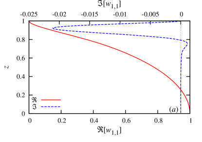
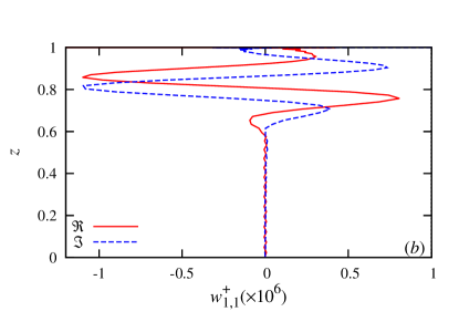
?figurename? 2: Real and imaginary parts of the critical perturbation $\hat{w}_{1,1}$ given by the right eigenvector $\boldsymbol{\mathsf{w}}_{1,1}$ (a) and those of the respective left eigenvector $\boldsymbol{\mathsf{w}}_{1,1}^{\dagger}$ (b).

We start with the Orr-Sommerfeld equation, whose collocation approximation

$$\boldsymbol{\mathsf{L}}_{1}(\lambda,\textit{Re}\bar{\boldsymbol{\mathsf{u}}})\boldsymbol{\mathsf{w}}_{1,1}=[\boldsymbol{\mathsf{M}}_{1}(\textit{Re}\bar{\boldsymbol{\mathsf{u}}})-\lambda\boldsymbol{\mathsf{A}}_{1}]\boldsymbol{\mathsf{w}}_{1,1}=\boldsymbol{\mathsf{0}},$$ (46)

after multiplication by $\boldsymbol{\mathsf{A}}_{1}^{-1},$ reduces to the standard complex matrix eigenvalue problem

$$[\boldsymbol{\mathsf{A}}_{1}^{-1}\boldsymbol{\mathsf{M}}_{1}(\textit{Re}\,\bar{\boldsymbol{\mathsf{u}}})-\lambda\boldsymbol{\mathsf{I}}]\boldsymbol{\mathsf{w}}_{1,1}=\boldsymbol{\mathsf{0}}.$$ (47)

The marginal Reynolds number $\textit{Re}_{0}$ for a given wave number $\alpha$ is determined by the condition $\Re[\lambda_{0}]=0$ for the eigenvalue $\lambda_{0}$ with the largest real part. Simultaneously with the right eigenvector $\boldsymbol{\mathsf{w}}_{1,1},$ we find also the associated left eigenvector $\boldsymbol{\mathsf{w}}_{1,1}^{\dagger}.$(Golub & van Loan, 1996) The right eigenvector is normalized using the condition (28), and the left one is normalized against the former using the complex vector dot product $\boldsymbol{\mathsf{w}}_{1,1}^{\dagger}\cdot\boldsymbol{\mathsf{w}}_{1,1}=1.$ This normalization simplifies subsequent expressions of Landau coefficients. Having found $\boldsymbol{\mathsf{w}}_{1,1}$ we can straightforwardly solve discretized counterparts of Eqs. (29) and (30), which yield the mean-flow perturbation $\boldsymbol{\mathsf{u}}_{0,2}$ and the complex amplitude distribution of the second harmonic $\boldsymbol{\mathsf{w}}_{2,2}.$ For the fixed flow rate considered later on, we shall need also the stream function of the mean-flow perturbation $\underline{\psi}_{0,2},$ which is obtained by solving collocation approximation of $\hat{\psi}_{0,2}^{\prime}=\hat{u}_{0,2}$ with the symmetry condition $\hat{\psi}_{0,2}(0)=0.$

Now, we can proceed to solving our final equation (31), whose collocation approximation can be written similarly to Eq. (46) as

$$\boldsymbol{\mathsf{L}}_{1}(\mathrm{i}\omega_{0},\textit{Re}_{0}\bar{\boldsymbol{\mathsf{u}}})\boldsymbol{\mathsf{w}}_{1,3}=\boldsymbol{\mathsf{F}}_{1}\boldsymbol{\mathsf{h}}_{1,3}^{w}+|A|^{-2}[\boldsymbol{\mathsf{F}}_{1}\boldsymbol{\mathsf{N}}_{1}(\textit{Re}_{2}\bar{\boldsymbol{\mathsf{u}}}+|A|^{2}\boldsymbol{\mathsf{u}}_{0,2})+\mathrm{i}\omega_{2}\boldsymbol{\mathsf{A}}_{1}]\boldsymbol{\mathsf{w}}_{1,1},$$ (48)

which represents a matrix eigenvalue perturbation problem. For this system of linear equation to be solvable, its r.h.s multiplied by $\boldsymbol{\mathsf{A}}_{1}^{-1},$ as in Eq. (47), has to be orthogonal to $\boldsymbol{\mathsf{w}}_{1,1}^{\dagger}.$(Hinch, 1991) This discrete solvability condition leads to the same reduced Landau equation (34), whose coefficients are now defined as

$$\mu_{1} = -\boldsymbol{\mathsf{w}}_{1,1}^{\dagger}\cdot\boldsymbol{\mathsf{A}}_{1}^{-1}\boldsymbol{\mathsf{F}}_{1}\boldsymbol{\mathsf{N}}_{1}(\bar{\boldsymbol{\mathsf{u}}})\boldsymbol{\mathsf{w}}_{1,1},$$ (49)

$$\mu_{2} = -\boldsymbol{\mathsf{w}}_{1,1}^{\dagger}\cdot\boldsymbol{\mathsf{A}}_{1}^{-1}\boldsymbol{\mathsf{F}}_{1}(\boldsymbol{\mathsf{N}}_{1}(\boldsymbol{\mathsf{u}}_{0,2})\boldsymbol{\mathsf{w}}_{1,1}+\boldsymbol{\mathsf{h}}_{1,3}^{w}).$$ (50)

Note that a similar projection onto the left eigenvector of discretized system is also used to construct reduced models in the flow control problems(Åkervik et al., 2007).

IV Validation of the method

In this section, the numerical method will be validated by computing the first Landau coefficient for plane Poiseuille flow which corresponds to $\textit{Ha}=0.$ Owing to the symmetry of the problem, both $\hat{w}_{1,1}$ and $\hat{u}_{0,2}$ are even, whereas $\hat{w}_{2,2}$ is an odd function of $z$. This allows us to search the solution only in the upper half of the layer which halves the number of required collocation points. $M=N/2=32$ collocation points in the half-channel is sufficient to obtain the critical Reynolds number $\textit{Re}_{c}=5772.22$, frequency $\omega_{c}=-1555.18$ and wave number $\alpha_{c}=1.02055$ to six significant figures.

The real and imaginary parts of the critical perturbation $\hat{w}_{1,1},$ which is given by the right eigenvector $\boldsymbol{\mathsf{w}}_{1,1},$ are plotted in Fig. 2 together with the respective left eigenvector $\boldsymbol{\mathsf{w}}_{1,1}^{\dagger}.$ Note that the latter is orthogonal to all other right eigenvectors but $\boldsymbol{\mathsf{w}}_{1,1},$ and has only a numerical but no physical meaning. Because of different inner product definitions for the continuous and discrete problems, $\boldsymbol{\mathsf{w}}_{1,1}^{\dagger}$ is also distinct from the adjoint eigenfunction $\hat{w}_{1,1}^{+}.$ Distributions of the mean-flow perturbation and that of the complex amplitude of the second harmonic in the top half of the layer are plotted in Fig. 3. Note that due to the non-standard scaling, our dimensionless frequency and velocity differ by a factor of $\textit{Re}_{c}$ from the values obtained with the conventional scaling based on the center-line velocity.

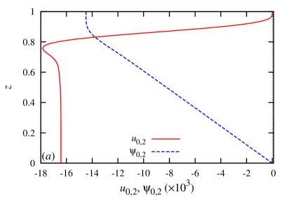
?figurename? 3: Velocity $\hat{u}_{0,2}$ and the associated stream function $\hat{\psi}_{0,2}$ of the mean-flow perturbation (a); the real and imaginary parts of the second harmonic amplitude $\hat{w}_{2,2}$ (b).

Substituting the above results into Eqs. (35) and (36) we obtain

$$\mu_{1} = 0.0097118-\mathrm{i}0.222596,$$

$$\mu_{2} = 0.0049382-\mathrm{i}0.0239131.$$

As seen from Fig. 4, $M\gtrsim 32$ collocation points produce Landau coefficients with about six significant figures. The first and most important result is $\Re[\mu_{2}]>0,$ which, as discussed above, confirms the subcritical nature of this instability in agreement with the previous studies. The linear growth rate coefficient $\mu_{1}$ has been computed explicitly by Stewartson & Stuart (1971), who found $d_{1}=(0.17+\mathrm{i}0.8)\times 10^{-5}$ for the standard normalization. Rescaling our result with the center-line velocity, we obtain $\tilde{\mu}_{1}=\mu_{1}/\textit{Re}_{c}=(0.168251-\mathrm{i}3.85633)\times 10^{-5},$ whose real part is close to that of $d_{1},$ while the imaginary part is significantly different. The reason for this difference is unclear. In addition, $\mu_{1}$ can be verified against the numerical results of linear stability analysis for the complex growth rate in the vicinity of the linear stability threshold, where $\delta\lambda=\lambda-\lambda_{c}\approx\mu_{1}(\textit{Re}-\textit{Re}_{c}).$ As seen in Fig. 5, the complex phase speed $c=-\mathrm{i}\lambda/\textit{Re}\,\alpha,$ which is commonly used instead of $\lambda,$ is accurately reproduced by $\mu_{1}$ in the vicinity of $\textit{Re}_{c}.$ This confirms the accuracy of $\mu_{1}$ found above.

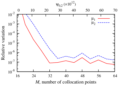
?figurename? 4: Relative variation of Landau coefficients with the number of collocation points $M.$

In order to compare our Landau coefficient $\mu_{2}$ with previous results, we have to take into account not only our non-standard normalization but also that $A$ in our case stands for the amplitude of the transverse velocity component $w,$ whereas in previous studies it denotes the amplitude of the stream function $\psi,$ which is related to the former by $\hat{w}=-\mathrm{i}\alpha\hat{\psi}.$ Thus, our $\mu_{2}$ rescales as

$$\tilde{\mu}_{2}=\mu_{2}\alpha_{c}^{2}\textit{Re}_{c}=29.659-\mathrm{i}143.622.$$

This result is close to $\tilde{\mu}_{2}=\mathrm{i}\alpha_{c}K_{1}=29.46-\mathrm{i}143.41$ found by Sen & Venkateswarlu (1983) using the method of Reynolds & Potter (1967) for $\textit{Re}_{c}=5774,$ $\alpha_{c}=1.02$ and $c_{r}=0.2639.$ Note that $K_{1}$ is mistaken for $\tilde{\mu}_{2}$ by Schmid & Henningson (2001), who denote it by $\lambda_{2}.$

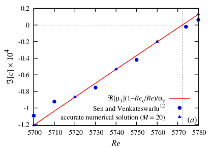
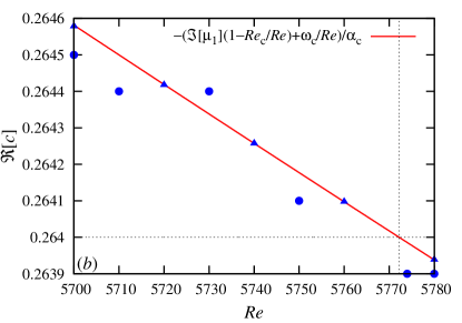
?figurename? 5: Imaginary (a) and real (b) parts of the complex phase velocity $c=-\mathrm{i}\lambda/\textit{Re}\,\alpha$ of the most unstable mode in the vicinity of the critical Reynolds number $\textit{Re}_{c}$ calculated using $\mu_{1}$ and supplied by the linear stability analysis (triangles) and taken from Sen & Venkateswarlu (1983) (circles).

Reynolds & Potter (1967) used their original method of “false solution” to obtain the first relatively accurate values of Landau coefficients for fixed flow rate. Our solution obtained for fixed pressure gradient can easily be converted into that for fixed flow rate by using the non-zero pressure gradient correction $P_{0,2}$ in Eq. (29). As seen from Eq. (26), this correction, which affects only the magnitude of the base flow, is equivalent to substituting $\textit{Re}_{2}$ by

$$\textit{Re}_{2}^{q}=\textit{Re}_{2}+|A|^{2}P_{0,2}/2.$$

Requiring the pressure correction $P_{0,2},$ which according to the expression above produces a flow rate perturbation $|A|^{2}P_{0,2}\bar{\psi}(1),$ to compensate $2|A|^{2}\hat{\psi}_{0,2}(1),$ which is the flow rate perturbation at fixed pressure gradient, we obtain

$$P_{0,2}/2=-\hat{\psi}_{0,2}(1)/\bar{\psi}(1)=0.00217238,$$

where $\bar{\psi}(1)=\int_{0}^{1}\bar{u}(z)\,dz=\frac{2}{3}.$ Thus, the substitution of $\textit{Re}_{2}$ by $\textit{Re}_{2}^{q}$ in Eq. (34) results in the replacement of $\mu_{2}$ by

$$\mu_{2}^{q}=\mu_{2}+\mu_{1}P_{0,2}/2=0.0051492-\mathrm{i}0.0287487.$$

Rescaling $\mu_{2}^{q}$ with the critical Reynolds number based on the mean velocity $\bar{\textit{Re}}_{c}=\frac{2}{3}\textit{Re}_{c}=3848.08$ and the critical wave number $\alpha_{c}=1.02071,$ which are the values used by Reynolds & Potter (1967), we have

$$\bar{\mu}_{2}^{q}=\mu_{2}^{q}\alpha_{c}^{2}\bar{\textit{Re}}_{c}=20.64-\mathrm{i}115.26,$$

which is close to $\bar{\mu}_{2}^{q}=a^{(2)}+\mathrm{i}b^{(2)}=19.7-\mathrm{i}111$ found by Reynolds & Potter (1967).

Alternatively, rescaling $\mu_{2}^{q}$ with $\textit{Re}_{c}$ based on the center-line velocity and the accurate value of $\alpha_{c},$ we obtain

$$\tilde{\mu}_{2}^{q}=\mu_{2}^{q}\alpha_{c}^{2}\textit{Re}_{c}=30.957-\mathrm{i}172.83,$$

which agrees well with $\tilde{\mu}_{2}=30.96126-\mathrm{i}172.8268$ and $\tilde{\mu}_{2}=30.95616-\mathrm{i}172.8335$ obtained respectively by the amplitude expansion using a highly accurate Chebyshev collocation method(Fujimura, 1989) and by the center manifold reduction using an expansion in linear eigenfunctions.(Fujimura, 1997)

V Results

V.1 Linear stability threshold of Hartmann flow

We start with revisiting the linear stability threshold of the Hartmann flow which is defined by the marginal Reynolds number at which perturbations with positive temporal growth rate $\Re[\lambda]$ appear. This Reynolds numbers and the associated phase velocity of neutrally stable modes are plotted in Fig. 6(a) versus the wave number $\alpha$ for several Hartmann numbers. The non-magnetic case $(\textit{Ha}=0)$ corresponds to the classic plane Poiseuille flow. First, it is seen that only the modes with sufficiently small wave numbers can be become linearly unstable. Second, each such a mode can be linearly unstable only in a limited range of Reynolds numbers. Namely, besides the lower marginal Reynolds number by exceeding which mode of a given wave number turns linearly unstable, there is also an upper marginal Reynolds number by exceeding which it becomes linearly stable. Linear stability threshold corresponds the lowest marginal Reynolds number which is referred to as the critical Reynolds number. For non-magnetic case $(\textit{Ha}=0)$, the critical Reynolds number is $\textit{Re}_{c}=5772.22,$ and it occurs at the critical wave number $\alpha_{c}=1.02055$.(Orszag, 1971) The former is seen in Fig. 6(a) to raise with the Hartmann number, which means that the flow is stabilized as the magnetic field is increased. The critical wave number first decreases and then starts to rise at $\textit{Ha}\gtrsim 2.$

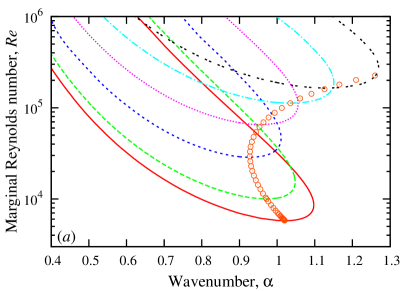
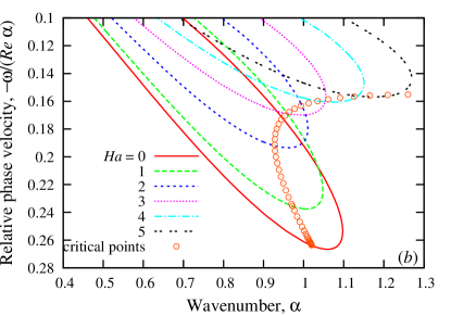
?figurename? 6: Marginal Reynolds number (a) and the relative phase velocities of neutrally stable modes (b) against wave number for various Hartmann numbers.

As seen in Fig. 7, the critical Reynolds number $\textit{Re}_{c}$ and the associated wave number $\alpha_{c}$ both increase in a sufficiently strong magnetic field $(\textit{Ha}\gtrsim 10)$ directly with the Hartmann number while the relative phase speed $c=-\omega/\textit{Re}\,\alpha$ tends to a constant. The best fit of the numerical results yield

$$\textit{Re}{}_{c} \sim 4.83\times 10^{4}\textit{Ha},$$ (51)

$$\alpha_{c} \sim 0.162\textit{Ha},$$ (52)

$$c_{c} \sim 0.155,$$ (53)

which agree well with the results of Takashima (1996). Note that besides the original instability mode, which develops from the non-magnetic one, another linearly unstable mode appears at $\textit{Ha}\gtrsim 6.5.$ At higher Hartmann numbers, the second mode closely approaches the original one. Both modes differ by their $z$-symmetry. The transverse velocity distribution is an even function of $z$ for the former and an odd function for the latter. This difference becomes unimportant when $\textit{Ha}\gtrsim 20.$ In such a strong magnetic field the instability becomes localized in the so-called Hartmann boundary layers of the characteristic thickness

$$\delta\sim h/\textit{Ha}.$$ (54)

First, the localization of instability is implied by the above variations of $\textit{Re}{}_{c}$ and $\alpha_{c},$ which both become independent of Ha when $\delta$ is used instead of $h$ as the characteristic length scale. Second, it is also confirmed by the streamline patterns of the critical perturbations for both modes which are seen in Fig. 8 to be very similar to each other. The perturbations differ by the direction of circulation in the vortices at the opposite walls, which is the same for the even mode and opposite for the odd mode. The co-rotating vortices in the even mode are connected through the mid-plane and, thus, enhance each other, whereas the counter-rotating vortices in the odd mode tend to suppress each other. In strong magnetic field, the vortices at the opposite walls become effectively separated by a stagnant liquid core which makes their interaction insignificant. This effect has implications for the subsequent weakly nonlinear analysis.

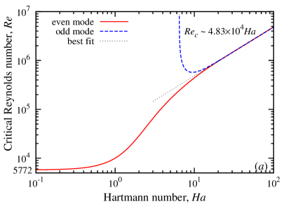
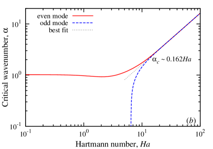
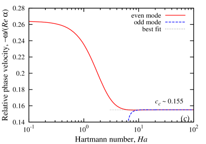
?figurename? 7: Critical Reynolds number (a), wave number (b) and phase speed (c) for even and odd instability modes against the Hartmann number.

?figurename? 8: Instantaneous streamlines of critical perturbations for even (a) and odd (b) modes at $\textit{Ha}=20.$

V.2 Weakly nonlinear subcritical equilibrium states

As noted above, the coefficients (35,36) and, thus, the equilibrium amplitude (37) determined by them depend on the normalization of linear eigenfunction. This is because the equilibrium perturbation (22), which is independent of the normalization, is given by the product of both quantities. For the classic plane Poiseuille flow, Landau coefficients are usually calculated by normalizing the linear eigenfunction at the middle of the layer by the condition (28). This standard normalization, however, is not suitable for the Hartmann flow. First, it is not compatible with the odd mode, which satisfies the symmetry condition $\hat{w}_{1,1}(0)=0.$ Second, as discussed above, the same condition is effectively satisfied also by the even mode when it becomes suppressed in the core of the layer by a sufficiently strong magnetic field. Thus, instead of the standard normalization condition (28), we use

$$\hat{w}_{1,1}^{\prime\prime}(1)=1,$$ (55)

which is related by Eq. (13) to the vorticity at the wall. This normalization condition is applicable to both even and odd modes regardless of the field strength.

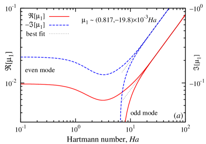
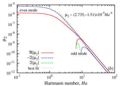
?figurename? 9: Linear growth rate coefficient $\mu_{1}$ (a) and and the first Landau coefficient $\mu_{2}$ (b) for odd and even instability modes normalized with (55).

The linear growth rate coefficient $\mu_{1}$ and the first Landau coefficient $\mu_{2}$ computed with this normalization condition for both critical modes are plotted in Fig. 9 against the Hartmann number. As seen from Eq. (34) these coefficients define the variation of the complex growth rate $\lambda_{2}=\mathrm{i}\omega_{2},$ where $\mu_{1}$ is associated with the deviation of Reynolds number from its linear stability threshold $\textit{Re}_{2},$ while $\mu_{2}$ accounts for the effect of amplitude $A.$ The real part of $\mu_{1}$ is positive because the critical mode becomes linearly unstable as Re exceeds $\textit{Re}_{c}.$ The positive $\Re[\mu_{2}],$ which is seen in Fig. 9(b) to be the case for all Hartmann numbers, means that the perturbation amplitude has a positive feedback on its growth rate. Consequently, the Hartmann flow is sub-critically unstable regardless of the magnetic field strength. For strong magnetic field $(\textit{Ha}\gtrsim 20)$, the best fit of numerical results yields

$$\mu_{1} \sim (0.814-\mathrm{i}19.8)\times 10^{-3}\textit{Ha},$$ (56)

$$\mu_{2} \sim (2.73-\mathrm{i}1.50)\times 10^{-5}\textit{Ha}^{-4}.$$ (57)

Substituting these asymptotics into Eq. (37) we obtain

$$|A|^{2}\sim 29.8\textit{Ha}^{5}(\textit{Re}_{c}-\textit{Re}).$$ (58)

The scaling above is consistent with the relevant length scale of instability determined by Eq. (54) which for our choice of the characteristic velocity $v_{\delta}=\nu/\delta$ leads to $A\sim w^{\prime\prime}\sim\textit{Ha}^{3}.$ The last result implies that the velocity of equilibrium perturbation increases asymptotically as $w\sim\textit{Ha},$ which is similar to the variation of $\textit{Re}_{c}$ with $\textit{Ha}.$ The coefficient in Eq. (58) differs from that found by Moresco & Alboussière (2003) because they normalize the fundamental mode using the velocity maximum, whereas we use the wall vorticity, which in contrast to the former is defined explicitly by Eq. (55).

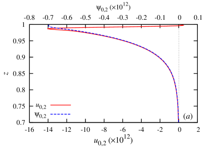
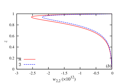
?figurename? 10: Velocity $\hat{u}_{0,2}=\hat{\psi}_{0,2}^{\prime}$ and the associated stream function $\hat{\psi}_{0,2}$ of the mean flow perturbation (a); the real and imaginary parts of the second harmonic amplitude $\hat{w}_{2,2}$ (b), and streamlines of the second-order perturbation (c) for the even mode at $\textit{Ha}=20.$

The perturbation of the mean flow $\hat{u}_{0,2}(z)$ and the complex amplitude distribution of the second harmonic $\hat{w}_{2,2}$, which both are produced by the nonlinear self-interaction of the fundamental harmonic, are plotted in Figs. 10(a,b). The perturbation of the flow rate is defined by the stream function $\hat{\psi}_{0,2}(z)=\int_{0}\hat{u}_{0,2}(z)\,dz.$ For strong magnetic field, the best fit yields

$$\hat{\psi}_{0,2}(1)\sim-4.45\times 10^{-5}\textit{Ha}^{-6},$$ (59)

whose product with $|A|^{2}$ defined by Eq. (58) according to Eq. (23) yields the dimensionless perturbation of the flow rate over half channel. Note that Ha cancels out in this product which is consistent with the dimensional arguments considered in the paragraph above. Similarly, one can define stream functions for higher harmonics which satisfy $w_{n}=-\partial_{x}\psi_{n}$ and, thus, lead to the following simple expressions for the complex amplitudes $\hat{\psi}_{n}=\mathrm{i}\alpha_{n}^{-1}\hat{w}_{n}.$ The streamlines of the second-order perturbation given by $\hat{\psi}_{0,2}(z)-\alpha_{c}^{-1}\Im[\hat{w}_{2,2}(z)\mathrm{e}^{\mathrm{i}2\alpha_{c}x}]$ are shown in Fig. 10(c) for the even mode near the upper wall at $\textit{Ha}=20.$ Note that the mean-flow perturbation at fixed pressure gradient reduces the total flow rate by the amount defined by Eq. (59). This reduction appears in Fig. 10(c) as the band of open streamlines undulating between the opposite vortices. The resulting equilibrium perturbation is formed by the superposition of this second-order perturbation with the amplitude $|A|{}^{2},$ which is defined by Eq. (58), and the critical perturbation with the amplitude $A$ and the streamline pattern shown in Fig. 8(a).

VI Conclusion

The present study was concerned with weakly nonlinear stability analysis of Hartmann flow, which is an MHD counterpart of plane Poiseuille flow. Using a non-standard but highly accurate and efficient numerical approach, which was validated on the classical plane Poiseuille flow, we computed the first Landau coefficient and the linear growth rate correction which determine weakly nonlinear evolution of finite small-amplitude disturbances in the vicinity of linear stability threshold. Hartmann flow was found to remain subcritically unstable in the whole range of the magnetic field strength. It means that finite amplitude disturbances can be become unstable at Reynolds numbers below the linear stability threshold of Hartmann flow. Next step is to determine how far these 2D as well as 3D finite-amplitude equilibrium states, which are expected to bifurcate from the former extend into the range of subcritical Reynolds numbers.(Ehrenstein & Koch, 1991) Such states are thought to mediate transition to turbulence in shear flows and thus may account for the low transition threshold observed in both experiments and direct numerical simulations.

The method we used for computing Landau coefficients differs from the standard one by the application of the solvability condition to the discretized rather than continuous problem. Expanding equilibrium solution in small perturbation amplitude in the vicinity of the linear stability threshold, we obtained a matrix eigenvalue perturbation problem for the transverse velocity component. Solvability of this problem requires its inhomogeneous term to be orthogonal to the left eigenvector. This nonstandard approach allowed us to bypass both the solution of the adjoint problem and the subsequent evaluation of the integrals defining the inner products, which resulted in a significant simplification of the method. The simplicity and relative accuracy of the method makes it potentially extendible to more complicated problems like that of MHD duct flow whose weakly nonlinear stability characteristics are still unclear.(Pothérat, 2007; Priede, Aleksandrova & Molokov, 2012)