Efficient Dimensionality Reduction for Canonical Correlation Analysis

Abstract

We present a fast algorithm for approximate Canonical Correlation Analysis (CCA). Given a pair of tall-and-thin matrices, the proposed algorithm first employs a randomized dimensionality reduction transform to reduce the size of the input matrices, and then applies any CCA algorithm to the new pair of matrices. The algorithm computes an approximate CCA to the original pair of matrices with provable guarantees, while requiring asymptotically less operations than the state-of-the-art exact algorithms.

1 Introduction

Canonical Correlation Analysis (CCA) [19] is an important technique in statistics, data analysis, and data mining. CCA has been successfully applied in many statistics and machine learning applications, e.g. dimensionality reduction [29], clustering [9], learning of word embeddings [12], sentiment classification [11], discriminant learning [28], and object recognition [21]. In many ways CCA is analogous to Principal Component Analysis (PCA), but instead of analyzing a single data-set (in matrix form), the goal of CCA is to analyze the relation between a pair of data-sets (each in matrix form). From a statistical point of view, PCA extracts the maximum covariance directions between elements in a single matrix, whereas CCA finds the direction of maximal correlation between a pair of matrices. From a linear algebraic point of view, CCA measures the similarities between two subspaces (those spanned by the columns of each of the two matrices analyzed). From a geometric point of view, CCA computes the cosine of the principle angles between the two subspaces.

There are different ways to define the canonical correlations of a pair of matrices, and all these methods are equivalent [16]. The linear algebraic formulation of Golub and Zha [16], which we present shortly, serves our algorithmic point of view best.

Definition 1.

Let ${\bm{\mathrm{A}}}\in\R^{m\times n}$ and ${\bm{\mathrm{B}}}\in\R^{m\times\ell}$ , and assume that $p=\hbox{\rm rank}({\bm{\mathrm{A}}})\geq\hbox{\rm rank}({\bm{\mathrm{B}}})=q$. The canonical correlations

$$\sigma_{1}\left({\bm{\mathrm{A}}},{\bm{\mathrm{B}}}\right)\geq\sigma_{2}\left({\bm{\mathrm{A}}},{\bm{\mathrm{B}}}\right)\geq\cdots\geq\sigma_{q}\left({\bm{\mathrm{A}}},{\bm{\mathrm{B}}}\right)$$

of the matrix pair $({\bm{\mathrm{A}}},{\bm{\mathrm{B}}})$ are defined recursively by the following formula:

$$\sigma_{i}\left({\bm{\mathrm{A}}},{\bm{\mathrm{B}}}\right)=\max_{{\mathbf{x}}\in{\cal A}_{i},{\mathbf{y}}\in{\cal B}_{i}}\sigma\left({\bm{\mathrm{A}}}{\mathbf{x}},{\bm{\mathrm{B}}}{\mathbf{y}}\right)=:\sigma\left({\bm{\mathrm{A}}}{\mathbf{x}}_{i},{\bm{\mathrm{B}}}{\mathbf{y}}_{i}\right),\quad i=1,\ldots,q$$

where

• $\sigma\left({\mathbf{u}},{\mathbf{v}}\right)=|{\mathbf{u}}^{\textsc{T}}{\mathbf{v}}|/\left(\mbox{}\|{\mathbf{u}}\|_{2}\mbox{}\|{\mathbf{v}}\|_{2}\right)$,

• ${\cal A}_{i}=\{{\mathbf{x}}:{\bm{\mathrm{A}}}{\mathbf{x}}\neq\bf{0},{\bm{\mathrm{A}}}{\mathbf{x}}\perp\{{\bm{\mathrm{A}}}{\mathbf{x}}_{1},\ldots,{\bm{\mathrm{A}}}{\mathbf{x}}_{i-1}\}\}$,

• ${\cal B}_{i}=\{{\mathbf{y}}:{\bm{\mathrm{B}}}{\mathbf{y}}\neq\bf{0},{\bm{\mathrm{B}}}{\mathbf{y}}\perp\{{\bm{\mathrm{B}}}{\mathbf{y}}_{1},\ldots,{\bm{\mathrm{B}}}{\mathbf{y}}_{i-1}\}\}$.

The unit vectors

$${\bm{\mathrm{A}}}{\mathbf{x}}_{1}/\mbox{}\|{\bm{\mathrm{A}}}{\mathbf{x}}_{1}\|_{2},\dots,{\bm{\mathrm{A}}}{\mathbf{x}}_{q}/\mbox{}\|{\bm{\mathrm{A}}}{\mathbf{x}}_{q}\|_{2},\quad and\quad{\bm{\mathrm{B}}}{\mathbf{y}}_{1}/\mbox{}\|{\bm{\mathrm{B}}}{\mathbf{y}}_{1}\|_{2},\dots,{\bm{\mathrm{B}}}{\mathbf{y}}_{q}/\mbox{}\|{\bm{\mathrm{B}}}{\mathbf{y}}_{q}\|_{2},$$

are called the canonical or principal vectors. The vectors

$${\mathbf{x}}_{1}/\mbox{}\|{\bm{\mathrm{A}}}{\mathbf{x}}_{1}\|_{2},\dots,{\mathbf{x}}_{q}/\mbox{}\|{\bm{\mathrm{A}}}{\mathbf{x}}_{q}\|_{2},\quad and\quad{\mathbf{y}}_{1}/\mbox{}\|{\bm{\mathrm{B}}}{\mathbf{y}}_{1}\|_{2},\dots,{\mathbf{y}}_{q}/\mbox{}\|{\bm{\mathrm{B}}}{\mathbf{y}}_{q}\|_{2},$$

are called canonical weights (or projection vectors). Note that the canonical weights and the canonical vectors are not uniquely defined.

1.1 Main Result

The main contribution of this article (see Theorem 15) is a fast algorithm to compute an approximate CCA. The algorithm computes an additive-error approximation to all the canonical correlations. It also computes a set of approximate canonical weights with provable guarantees. We show that the proposed algorithm is asymptotically faster compared to the standard method of Björck and Golub [5]. To the best of our knowledge, this is the first sub-cubic time algorithm for approximate CCA that has provable guarantees.

The proposed algorithm is based on dimensionality reduction: given a pair of matrices $({\bm{\mathrm{A}}},{\bm{\mathrm{B}}})$, we transform the pair to a new pair $(\hat{{\bm{\mathrm{A}}}},\hat{{\bm{\mathrm{B}}}})$ that has much fewer rows, and then compute the canonical correlations of the new pair exactly, alongside a set of canonical weights, e.g. using the Björck and Golub algorithm. We prove that with high probability the canonical correlations of $(\hat{{\bm{\mathrm{A}}}},\hat{{\bm{\mathrm{B}}}})$ are close to the canonical correlations of $({\bm{\mathrm{A}}},{\bm{\mathrm{B}}})$, and that any set of canonical weights of $(\hat{{\bm{\mathrm{A}}}},\hat{{\bm{\mathrm{B}}}})$ can be used to construct a set of approximately orthogonal canonical vectors of $(\hat{{\bm{\mathrm{A}}}},\hat{{\bm{\mathrm{B}}}})$. The transformation of $({\bm{\mathrm{A}}},{\bm{\mathrm{B}}})$ into $(\hat{{\bm{\mathrm{A}}}},\hat{{\bm{\mathrm{B}}}})$ is done in two steps. First, we apply the Randomized Walsh-Hadamard Transform (RHT) to both ${\bm{\mathrm{A}}}$ and ${\bm{\mathrm{B}}}$. This is a unitary transformation, so the canonical correlations are preserved exactly. On the other hand, we show that with high probability, the transformed matrices have their “information” equally spread among all the input rows, so now the transformed matrices are amenable to uniform sampling. In the second step, we uniformly sample (without replacement) a sufficiently large set of rows and rescale them to form $(\hat{{\bm{\mathrm{A}}}},\hat{{\bm{\mathrm{B}}}})$. The combination of RHT and uniform sampling is often called Subsampled Randomized Walsh-Hadamard Transform (SRHT) in the literature [32]. Note that other variants of dimensionality reduction [26] might be appropriate as well, but for concreteness we focus on the SRHT (see also Section 6).

Our dimensionality reduction scheme is particularly effective when the matrices are tall-and-thin, that is they have much more rows than columns. Targeting such matrices is natural: in typical CCA applications, columns typically correspond to features or labels and rows correspond to samples or training data. By computing the CCA on as many instances as possible (as much training data as possible), we get the most reliable estimates of application-relevant quantities. However in current algorithms adding instances (rows) is expensive, e.g. in Björck and Golub algorithm we pay $O(n^{2}+\ell^{2})$ for each row. Our algorithm allows practitioners to run CCA on huge data sets because we reduce the cost of an extra row to almost $O(n+\ell)$.

We also discuss a variant of our dimensionality reduction scheme that is more suitable for sparse matrices (Section 6), and show that it is not possible to replace the additive error guarantees in our analysis with relative error guarantees (Section 7). Finally, we demonstrate that our algorithm is faster than the standard algorithm in practice by 30-60% even on fairly small matrices (Section 8).

1.2 Related Work

Dimensionality reduction has been the driving force behind many recent algorithms for accelerating key machine learning and linear algebraic tasks. A representative example is linear regression, i.e., solve the least squares problem $\min_{{\mathbf{x}}}\mbox{}\|{\bm{\mathrm{A}}}{\mathbf{x}}-{\mathbf{b}}\|_{2}$, where ${\mathbf{b}}\in\R^{m}$. If $m\gg n$, then one can use the SRHT to reduce the dimension of ${\bm{\mathrm{A}}}$ and ${\mathbf{b}}$, to form $\hat{{\bm{\mathrm{A}}}}$ and $\hat{{\mathbf{b}}}$, and then solve the small problem $\min_{{\mathbf{x}}}\mbox{}\|\hat{{\bm{\mathrm{A}}}}{\mathbf{x}}-\hat{{\mathbf{b}}}\|_{2}$. This process will return an approximate solution to the original problem [26, 6, 14]. Alternatively, one can observe that ${\bm{\mathrm{A}}}^{\textsc{T}}{\bm{\mathrm{A}}}$ and $\hat{{\bm{\mathrm{A}}}}^{\textsc{T}}\hat{{\bm{\mathrm{A}}}}$ are spectrally close, so $\hat{{\bm{\mathrm{A}}}}$ is an effective preconditioner for ${\bm{\mathrm{A}}}$ [25, 3]. Other problems that can be accelerated using dimensionality reduction include: (i) approximate PCA (via low-rank matrix approximation) [17]; (ii) matrix multiplication [26]; (iii) K-means clustering [7]; (iv) approximation of matrix coherence and statistical leverage [13]; to name only a few.

Our approach uses similar techniques as the algorithms mentioned above. For example, Lemma 4 plays a central role in these algorithms as well. However, our analysis requires the use of advanced ideas from matrix perturbation theory and it leads to two new technical lemmas that might be of independent interest: Lemmas 10 and 11 provide bounds for the singular values of the product of two different sampled orthonormal matrices. Previous work only provides bounds for products of the same matrix (Lemma 4; see also [26, Corollary 11])

Dimensionality reduction techniques for accelerating CCA have been suggested or used in the past. One common technique is to simply use less samples by uniformly sampling the rows. Although this technique might work reasonably well in many instances, it may fail for others unless all rows are sampled. In fact, Theorem 13 analyzes uniform sampling, and establishes bounds on the required sample size.

Sun et al. suggest a two-stage approach which involves first solving a least-squares problem, and then using the solution to reduce the problem size [29]. However, their technique involves explicitly factoring one of the two matrices, which takes cubic time. Therefore, their method is especially effective when one of the two matrices has significantly less columns than the other. When the two matrices have about the same number of columns, there is no asymptotic performance gain. In contrast, our method is sub-cubic in any case.

Finally, it is worth noting that CCA itself has been used for dimensionality reduction [30, 9, 29]. This is not the focus of this article; we suggest a dimensionality reduction technique to accelerate CCA.

2 Preliminaries

We use $i:j$ to denote the set $\{i,\dots,j\}$, and $[n]=1:n$. We use ${\bm{\mathrm{A}}},{\bm{\mathrm{B}}},\ldots$ to denote matrices and ${\mathbf{a}},{\mathbf{b}},\ldots$ to denote column vectors. ${\bm{\mathrm{I}}}_{n}$ is the $n\times n$ identity matrix; $\bm{0}_{m\times n}$ is the $m\times n$ matrix of zeros. We denote the number of non-zero elements in ${\bm{\mathrm{A}}}$ by ${\rm nnz}({\bm{\mathrm{A}}})$. We denote by $\mathcal{R}(\cdot)$ the column space of its argument matrix. We denote by $[{\bm{\mathrm{A}}};{\bm{\mathrm{B}}}]$ the matrix obtained by concatenating the columns of ${\bm{\mathrm{B}}}$ next to the columns of ${\bm{\mathrm{A}}}$. Given a subset of indices $T\subseteq[m]$, the corresponding sampling matrix ${\bm{\mathrm{S}}}$ is the $|T|\times m$ matrix obtained by discarding from ${\bm{\mathrm{I}}}_{m}$ the rows whose index is not in $T$. Note that ${\bm{\mathrm{S}}}{\bm{\mathrm{A}}}$ is the matrix obtained by keeping only the rows in ${\bm{\mathrm{A}}}$ whose index appears in $T$. A symmetric matrix ${\bm{\mathrm{A}}}$ is positive semi-definite (PSD), denoted by $0\preceq{\bm{\mathrm{A}}}$, if ${\mathbf{x}}^{\textsc{T}}{\bm{\mathrm{A}}}{\mathbf{x}}\geq 0$ for every vector ${\mathbf{x}}$. For any two symmetric matrices ${\bm{\mathrm{X}}}$ and ${\bm{\mathrm{Y}}}$ of the same size, ${\bm{\mathrm{X}}}\preceq{\bm{\mathrm{Y}}}$ denotes that ${\bm{\mathrm{Y}}}-{\bm{\mathrm{X}}}$ is a PSD matrix.

We denote the compact (or thin) SVD of a matrix ${\bm{\mathrm{A}}}\in\R^{m\times n}$ of rank $p$ by ${\bm{\mathrm{A}}}={\bm{\mathrm{U}}}_{{\bm{\mathrm{A}}}}{\bm{\mathrm{\Sigma}}}_{\bm{\mathrm{A}}}{\bm{\mathrm{V}}}_{\bm{\mathrm{A}}}^{\textsc{T}}$, with ${\bm{\mathrm{U}}}_{{\bm{\mathrm{A}}}}\in\R^{m\times p}$, ${\bm{\mathrm{\Sigma}}}_{\bm{\mathrm{A}}}\in\R^{p\times p}$, and ${\bm{\mathrm{V}}}_{\bm{\mathrm{A}}}^{\textsc{T}}\in\R^{p\times n}$. The Moore-Penrose pseudo-inverse of ${\bm{\mathrm{A}}}$ is ${{\bm{\mathrm{A}}}}^{+}={\bm{\mathrm{V}}}_{\bm{\mathrm{A}}}{\bm{\mathrm{\Sigma}}}_{\bm{\mathrm{A}}}^{-1}{\bm{\mathrm{U}}}_{\bm{\mathrm{A}}}^{\textsc{T}}\in\R^{n\times m}$. We denote the singular values of ${\bm{\mathrm{A}}}$ by $\sigma_{1}({\bm{\mathrm{A}}})\geq\sigma_{2}({\bm{\mathrm{A}}})\geq\dots\geq\sigma_{p}({\bm{\mathrm{A}}})$.

2.1 The Björck and Golub Algorithm

There are quite a few algorithms to compute the canonical correlations [16]. One of the most popular methods is due to Björck and Golub [5]. It is based on the following observation.

Theorem 2 ([5]).

Assume that the columns of ${\bm{\mathrm{Q}}}\in\R^{m\times p}$ ($m\geq p$) and ${\bm{\mathrm{W}}}\in\R^{m\times q}$ ($m\geq q$) form an orthonormal basis for the range of ${\bm{\mathrm{A}}}$ and ${\bm{\mathrm{B}}}$ (respectively). Let ${\bm{\mathrm{Q}}}^{\textsc{T}}{\bm{\mathrm{W}}}={\bm{\mathrm{U}}}{\bm{\mathrm{\Sigma}}}{\bm{\mathrm{V}}}^{\textsc{T}}$ be its compact SVD. The diagonal elements of ${\bm{\mathrm{\Sigma}}}$ are the canonical correlations of $({\bm{\mathrm{A}}},{\bm{\mathrm{B}}})$. The canonical vectors are given by the first $q$ columns of ${\bm{\mathrm{Q}}}{\bm{\mathrm{U}}}$ (for ${\bm{\mathrm{A}}}$) and ${\bm{\mathrm{W}}}{\bm{\mathrm{V}}}$ (for ${\bm{\mathrm{B}}}$).

Theorem 2 implies that once we have a pair of matrices ${\bm{\mathrm{Q}}}$ and ${\bm{\mathrm{W}}}$ with orthonormal columns whose column space spans the same column space of ${\bm{\mathrm{A}}}$ and ${\bm{\mathrm{B}}}$, respectively, then all we need is to compute the singular value decomposition of ${\bm{\mathrm{Q}}}^{\textsc{T}}{\bm{\mathrm{W}}}$. Björck and Golub suggest the use of QR decompositions, but ${\bm{\mathrm{U}}}_{\bm{\mathrm{A}}}$ and ${\bm{\mathrm{U}}}_{\bm{\mathrm{B}}}$ will serve as well. Both options require $O\left(m\left(n^{2}+\ell^{2}\right)\right)$ time.

Corollary 3.

Frame Definition 1. Let ${\bm{\mathrm{U}}}^{\textsc{T}}_{\bm{\mathrm{A}}}{\bm{\mathrm{U}}}_{\bm{\mathrm{B}}}={\bm{\mathrm{U}}}{\bm{\mathrm{\Sigma}}}{\bm{\mathrm{V}}}^{\textsc{T}}$ be the compact SVD of ${\bm{\mathrm{U}}}^{\textsc{T}}_{\bm{\mathrm{A}}}{\bm{\mathrm{U}}}_{\bm{\mathrm{B}}}$. Then, for $i\in[q]$: $\sigma_{i}({\bm{\mathrm{A}}},{\bm{\mathrm{B}}})={\bm{\mathrm{\Sigma}}}_{ii}$. The canonical weights are given by the columns of ${\bm{\mathrm{V}}}_{\bm{\mathrm{A}}}{\bm{\mathrm{\Sigma}}}^{-1}_{{\bm{\mathrm{A}}}}{\bm{\mathrm{U}}}$ (for ${\bm{\mathrm{A}}}$) and ${\bm{\mathrm{V}}}_{\bm{\mathrm{B}}}{\bm{\mathrm{\Sigma}}}^{-1}_{{\bm{\mathrm{B}}}}{\bm{\mathrm{V}}}$ (for ${\bm{\mathrm{B}}}$).

2.2 Matrix Coherence and Sampling from an Orthonormal Matrix

Matrix coherence is a fundamental concept in the analysis of matrix sampling algorithms (e.g. [31, 20]). There a quite a few similar but different ways to define the coherence. In this article we use the following definition. Given a matrix ${\bm{\mathrm{A}}}$ with $m$ rows, the coherence of ${\bm{\mathrm{A}}}$ is defined as

$$\mu({\bm{\mathrm{A}}})=\max_{i\in{[m]}}\mbox{}\|{\mathbf{e}}_{i}^{\top}{\bm{\mathrm{U}}}_{{\bm{\mathrm{A}}}}\|_{2}^{2},$$

where ${\mathbf{e}}_{i}$ is the $i$-th standard basis (column) vector of $\R^{m}$. Note that the coherence of ${\bm{\mathrm{A}}}$ is a property of the column space of ${\bm{\mathrm{A}}}$, and does not depend on the actual choice of ${\bm{\mathrm{A}}}$. Therefore, if $\mathcal{R}({\bm{\mathrm{A}}})=\mathcal{R}({\bm{\mathrm{B}}})$ then $\mu({\bm{\mathrm{A}}})=\mu({\bm{\mathrm{B}}})$. Furthermore, it is easy to verify that if $\mathcal{R}({\bm{\mathrm{A}}})\subseteq\mathcal{R}({\bm{\mathrm{B}}})$ then $\mu({\bm{\mathrm{A}}})\leq\mu({\bm{\mathrm{B}}})$. Finally, we mention that for every matrix ${\bm{\mathrm{A}}}$ with $m$ rows: $\hbox{\rm rank}({\bm{\mathrm{A}}})/m\leq\mu({\bm{\mathrm{A}}})\leq 1.$

We focus on tall-and-thin matrices, i.e. matrices with (much) more rows than columns. We are interested in dimensionality reduction techniques that (approximately) preserve the singular values of the original matrix. The simplest idea to do dimensionality reduction in tall-and-thin matrices is uniform sampling of the rows of the matrix. Coherence measures how susceptible the matrix is to uniform sampling; the following lemma shows that not too many samples are required when the coherence is small. The bound is almost tight [32, Section 3.3].

Lemma 4 (Sampling from Orthonormal Matrix, Corollary to Lemma 3.4 from [32]).

Let ${\bm{\mathrm{Q}}}\in\R^{m\times d}$ have orthonormal columns. Let $0<\epsilon<1$ and $0<\delta<1$. Let $r$ be an integer such that

$$6\epsilon^{-2}m\mu({\bm{\mathrm{Q}}})\log(3d/\delta)\leq r\leq m\,.$$

Let $T$ be a random subset of $[m]$ of cardinality $r$, drawn from a uniform distribution over such subsets, and let ${\bm{\mathrm{S}}}$ be the $|T|\times m$ sampling matrix corresponding to $T$ rescaled by $\sqrt{m/r}$. Then, with probability of at least $1-\delta$, for $i\in[d]$: $\sqrt{1-\epsilon}\leq\sigma_{i}({\bm{\mathrm{S}}}{\bm{\mathrm{Q}}})\leq\sqrt{1+\epsilon}.$

Proof.

Apply Lemma 3.4 from [32] with the following choice of parameters: $\ell=\alpha M\log(k/\delta),$ $\alpha=6/\epsilon^{2},$ and $\delta_{tropp}=\eta=\epsilon$. Here, $\ell$, $\alpha$, $M$, $k$, $\eta$ are the parameters of Lemma 3.4 from [32]; also $\delta_{tropp}$ plays the role of $\delta$, an error parameter, of Lemma 3.4 from [32]. $\epsilon$ and $\delta$ are from our Lemma.  

In the above lemma, $T$ is obtained by sampling coordinates from $[m]$ without replacement. Similar results can be shown for sampling with replacement, or using Bernoulli variables [20].

2.3 Randomized Fast Unitary Transforms

Matrices with high coherence pose a problem for algorithms based on uniform row sampling. One way to circumvent this problem is to use a coherence-reducing transformation. It is important that this transformation will not change the solution to the problem.

One popular coherence-reducing method is applying a randomized fast unitary transform. The crucial observation is that many problems can be safely transformed using unitary matrices. This is also true for CCA: $\sigma_{i}({\bm{\mathrm{Q}}}{\bm{\mathrm{A}}},{\bm{\mathrm{Q}}}{\bm{\mathrm{B}}})=\sigma_{i}({\bm{\mathrm{A}}},{\bm{\mathrm{B}}})$ if ${\bm{\mathrm{Q}}}$ is unitary (i.e., ${\bm{\mathrm{Q}}}^{\textsc{T}}{\bm{\mathrm{Q}}}$ is equal to the identity matrix). If the unitary matrix is chosen carefully, it can reduce the coherence. However, any fixed unitary matrix will fail to reduce the coherence on some matrices.

The solution is to couple a fixed unitary transform with some randomization. More specifically, the construction is ${\cal F}={\bm{\mathrm{F}}}{\bm{\mathrm{D}}}\,$, where ${\bm{\mathrm{D}}}$ is a random diagonal matrix of size $m$ whose entries are independent random signs, and ${\bm{\mathrm{F}}}$ is some fixed unitary matrix. An important quantity is the maximum squared element in ${\bm{\mathrm{F}}}$ (we denote this quantity with $\eta$): for any fixed ${\bm{\mathrm{X}}}\in\R^{n\times m}$ it can be shown that with constant probability, $\mu({\cal F}{\bm{\mathrm{X}}})\leq O\left(\eta n\log(m)\right)$ [3]. So, it is important for $\eta$ to be small. It is also necessary that ${\bm{\mathrm{F}}}$ can be applied quickly to ${\bm{\mathrm{X}}}$. FFT and FFT-like transforms have both these properties, and work well in practice due to the availability of high quality implementations.

Another fast unitary transform that has the above two properties is the Walsh-Hadamard Transform (WHT), which is defined as follows. Fix an integer $m=2^{h}$, for $h=1,2,3,\ldots$. The (non-normalized) $m\times m$ matrix of the Walsh-Hadamard Transform (WHT) is defined recursively as,

$${\bm{\mathrm{H}}}_{m}=\left[\begin{array}[]{cc}{\bm{\mathrm{H}}}_{m/2}&{\bm{\mathrm{H}}}_{m/2}\\ {\bm{\mathrm{H}}}_{m/2}&-{\bm{\mathrm{H}}}_{m/2}\end{array}\right],\ \mbox{with}\ {\bm{\mathrm{H}}}_{2}=\left[\begin{array}[]{cc}+1&+1\\ +1&-1\end{array}\right].$$

The $m\times m$ normalized matrix of the Walsh-Hadamard transform is ${\bm{\mathrm{H}}}=m^{-{1\over 2}}{\bm{\mathrm{H}}}_{m}$.

The recursive nature of the WHT allows us to compute ${\bm{\mathrm{H}}}{\bm{\mathrm{X}}}$ for an $m\times n$ matrix ${\bm{\mathrm{X}}}$ in time $O(mn\log(m))$. However, in our case we are interested in ${\bm{\mathrm{S}}}{\bm{\mathrm{H}}}{\bm{\mathrm{X}}}$ where ${\bm{\mathrm{S}}}$ is a $r$-row sampling matrix. To compute ${\bm{\mathrm{S}}}{\bm{\mathrm{H}}}{\bm{\mathrm{X}}}$ only $O(mn\log(r))$ operations suffice [2, Theorem 2.1].

Combining the WHT with a random diagonal sign matrix is called the Randomized Walsh-Hadamard Transform (RHT)

Definition 5 (Randomized Walsh-Hadamard Transform (RHT)).

Let $m=2^{h}$ for some positive integer $h$. A Randomized Walsh-Hadamard Transform (RHT) is an $m\times m$ matrix of the form

$${\bm{\mathrm{\Theta}}}={\bm{\mathrm{H}}}{\bm{\mathrm{D}}}\,$$

where ${\bm{\mathrm{D}}}$ is a random diagonal matrix of size $m$ whose entries are independent random signs, and ${\bm{\mathrm{H}}}$ is a normalized Walsh-Hadamard matrix of size $m$.

For concreteness, our analysis uses the RHT since it has the tightest coherence reducing bound. Our results generalize to other randomized fast unitary transforms, perhaps with some slightly different bounds.

Lemma 6 (RHT bounds Coherence, Lemma 3.3 from [32]).

Let ${\bm{\mathrm{A}}}$ be an $m\times n$ ($m\geq n$, $m=2^{h}$ for some positive integer $h$) matrix, and let ${\bm{\mathrm{\Theta}}}$ be an RHT. Then, with probability of at least $1-\delta$,

$$\mu({\bm{\mathrm{\Theta}}}{\bm{\mathrm{A}}})\leq{1\over m}\left(\sqrt{n}+\sqrt{8\log(m/\delta)}\right)^{2}\,.$$

3 Perturbation Bounds for Matrix Products

This section states three new technical lemmas which analyze the perturbation of the singular values of the product of a pair of matrices after dimensionality reduction. These lemmas are essential for our analysis in subsequent sections, but they might be of independent interest as well. We first state three well known results.

Lemma 7 ([15] Theorem 3.3).

Let ${\bm{\mathrm{\Psi}}}\in\R^{p\times q}$ and ${\bm{\mathrm{\Phi}}}={\bm{\mathrm{D}}}_{{\bm{\mathrm{L}}}}{\bm{\mathrm{\Psi}}}{\bm{\mathrm{D}}}_{{\bm{\mathrm{R}}}}$ with ${\bm{\mathrm{D}}}_{{\bm{\mathrm{L}}}}\in\R^{p\times p}$ and ${\bm{\mathrm{D}}}_{{\bm{\mathrm{R}}}}\in\R^{q\times q}$ being non-singular matrices. Let

$$\gamma=\max\{\mbox{}\|{\bm{\mathrm{D}}}_{{\bm{\mathrm{L}}}}{\bm{\mathrm{D}}}_{{\bm{\mathrm{L}}}}^{\textsc{T}}-{\bm{\mathrm{I}}}_{p}\|_{2},\mbox{}\|{\bm{\mathrm{D}}}_{{\bm{\mathrm{R}}}}^{\textsc{T}}{\bm{\mathrm{D}}}_{{\bm{\mathrm{R}}}}-{\bm{\mathrm{I}}}_{q}\|_{2}\}.$$

Then, for all $i=1,\ldots,\hbox{\rm rank}({\bm{\mathrm{\Psi}}}):$ $|\sigma_{i}\left({\bm{\mathrm{\Phi}}}\right)-\sigma_{i}\left({\bm{\mathrm{\Psi}}}\right)|\leq\gamma\cdot\sigma_{i}\left({\bm{\mathrm{\Psi}}}\right).$

Lemma 8 (Weyl’s inequality for singular values; [18] Corollary 7.3.8).

Let ${\bm{\mathrm{\Phi}}},{\bm{\mathrm{\Psi}}}\in\R^{m\times n}$. Then, for all $i=1,\ldots,\min(m,n):$

$$|\sigma_{i}\left({\bm{\mathrm{\Phi}}}\right)-\sigma_{i}\left({\bm{\mathrm{\Psi}}}\right)|\leq\mbox{}\|{\bm{\mathrm{\Phi}}}-{\bm{\mathrm{\Psi}}}\|_{2}.$$

Lemma 9 (Conjugating the PSD ordering; Observation 7.7.2 in [18]).

Let ${\bm{\mathrm{\Phi}}},{\bm{\mathrm{\Psi}}}\in\R^{n\times n}$ be symmetric matrices with ${\bm{\mathrm{\Phi}}}\preceq{\bm{\mathrm{\Psi}}}$. Then, for every $n\times m$ matrix ${\bm{\mathrm{Z}}}:$

$${\bm{\mathrm{Z}}}^{\textsc{T}}{\bm{\mathrm{\Phi}}}{\bm{\mathrm{Z}}}\preceq{\bm{\mathrm{Z}}}^{\textsc{T}}{\bm{\mathrm{\Psi}}}{\bm{\mathrm{Z}}}.$$

We now present the new technical lemmas.

Lemma 10.

Let ${\bm{\mathrm{A}}}\in\R^{m\times n}$ ($m\geq n$) and ${\bm{\mathrm{B}}}\in\R^{m\times\ell}$ ($m\geq\ell$). Define ${\bm{\mathrm{C}}}:=[{\bm{\mathrm{A}}};{\bm{\mathrm{B}}}]\in\R^{m\times(n+\ell)}$, and suppose ${\bm{\mathrm{C}}}$ has rank $\omega$, so ${\bm{\mathrm{U}}}_{{\bm{\mathrm{C}}}}\in\R^{m\times\omega}$. Let ${\bm{\mathrm{S}}}\in\R^{r\times m}$ be any matrix such that

$$\sqrt{1-\epsilon}\leq\sigma_{\omega}\left({\bm{\mathrm{S}}}{\bm{\mathrm{U}}}_{{\bm{\mathrm{C}}}}\right)\leq\sigma_{1}\left({\bm{\mathrm{S}}}{\bm{\mathrm{U}}}_{{\bm{\mathrm{C}}}}\right)\leq\sqrt{1+\epsilon},$$

for some $0<\epsilon<1$ . Then, for $i=1,\dots,\min(n,\ell)$,

$$|\sigma_{i}\left({\bm{\mathrm{A}}}^{\textsc{T}}{\bm{\mathrm{B}}}\right)-\sigma_{i}\left({\bm{\mathrm{A}}}^{\textsc{T}}{\bm{\mathrm{S}}}^{\textsc{T}}{\bm{\mathrm{S}}}{\bm{\mathrm{B}}}\right)|\leq\epsilon\cdot\mbox{}\|{\bm{\mathrm{A}}}\|_{2}\cdot\mbox{}\|{\bm{\mathrm{B}}}\|_{2}\,.$$

Proof.

Using Weyl’s inequality for the singular values of arbitrary matrices (Lemma 8) we obtain,

$$|\sigma_{i}\left({\bm{\mathrm{A}}}^{\textsc{T}}{\bm{\mathrm{B}}}\right)-\sigma_{i}\left({\bm{\mathrm{A}}}^{\textsc{T}}{\bm{\mathrm{S}}}^{\textsc{T}}{\bm{\mathrm{S}}}{\bm{\mathrm{B}}}\right)| \leq \mbox{}\|{\bm{\mathrm{A}}}^{\textsc{T}}{\bm{\mathrm{S}}}^{\textsc{T}}{\bm{\mathrm{S}}}{\bm{\mathrm{B}}}-{\bm{\mathrm{A}}}^{\textsc{T}}{\bm{\mathrm{B}}}\|_{2}$$

$$= \mbox{}\|{\bm{\mathrm{V}}}_{{\bm{\mathrm{A}}}}{\bm{\mathrm{\Sigma}}}_{{\bm{\mathrm{A}}}}\left({\bm{\mathrm{U}}}_{{\bm{\mathrm{A}}}}^{\textsc{T}}{\bm{\mathrm{S}}}^{\textsc{T}}{\bm{\mathrm{S}}}{\bm{\mathrm{U}}}_{{\bm{\mathrm{B}}}}-{\bm{\mathrm{U}}}_{{\bm{\mathrm{A}}}}^{\textsc{T}}{\bm{\mathrm{U}}}_{{\bm{\mathrm{B}}}}\right){\bm{\mathrm{\Sigma}}}_{{\bm{\mathrm{B}}}}{\bm{\mathrm{V}}}^{\textsc{T}}_{{\bm{\mathrm{B}}}}\|_{2}$$

$$\leq \mbox{}\|{\bm{\mathrm{U}}}_{{\bm{\mathrm{A}}}}^{\textsc{T}}{\bm{\mathrm{S}}}^{\textsc{T}}{\bm{\mathrm{S}}}{\bm{\mathrm{U}}}_{{\bm{\mathrm{B}}}}-{\bm{\mathrm{U}}}_{{\bm{\mathrm{A}}}}^{\textsc{T}}{\bm{\mathrm{U}}}_{{\bm{\mathrm{B}}}}\|_{2}\cdot\mbox{}\|{\bm{\mathrm{A}}}\|_{2}\cdot\mbox{}\|{\bm{\mathrm{B}}}\|_{2}\,.$$

Next, we argue that $\mbox{}\|{\bm{\mathrm{U}}}_{{\bm{\mathrm{A}}}}^{\textsc{T}}{\bm{\mathrm{S}}}^{\textsc{T}}{\bm{\mathrm{S}}}{\bm{\mathrm{U}}}_{{\bm{\mathrm{B}}}}-{\bm{\mathrm{U}}}_{{\bm{\mathrm{A}}}}^{\textsc{T}}{\bm{\mathrm{U}}}_{{\bm{\mathrm{B}}}}\|_{2}\leq\mbox{}\|{\bm{\mathrm{U}}}_{{\bm{\mathrm{C}}}}^{\textsc{T}}{\bm{\mathrm{S}}}^{\textsc{T}}{\bm{\mathrm{S}}}{\bm{\mathrm{U}}}_{{\bm{\mathrm{C}}}}-{\bm{\mathrm{I}}}_{\omega}\|_{2}$. Indeed, we now have

$$\mbox{}\|{\bm{\mathrm{U}}}_{{\bm{\mathrm{A}}}}^{\textsc{T}}{\bm{\mathrm{S}}}^{\textsc{T}}{\bm{\mathrm{S}}}{\bm{\mathrm{U}}}_{{\bm{\mathrm{B}}}}-{\bm{\mathrm{U}}}_{{\bm{\mathrm{A}}}}^{\textsc{T}}{\bm{\mathrm{U}}}_{{\bm{\mathrm{B}}}}\|_{2} = \sup_{\mbox{}\|{\mathbf{w}}\|_{2}=1,\ \mbox{}\|{\mathbf{z}}\|_{2}=1}|{\mathbf{w}}^{\textsc{T}}{\bm{\mathrm{U}}}_{{\bm{\mathrm{A}}}}^{\textsc{T}}{\bm{\mathrm{S}}}^{\textsc{T}}{\bm{\mathrm{S}}}{\bm{\mathrm{U}}}_{{\bm{\mathrm{B}}}}{\mathbf{z}}-{\mathbf{w}}^{\textsc{T}}{\bm{\mathrm{U}}}_{{\bm{\mathrm{A}}}}^{\textsc{T}}{\bm{\mathrm{U}}}_{{\bm{\mathrm{B}}}}{\mathbf{z}}|$$

$$= \sup_{\mbox{}\|{\mathbf{x}}\|_{2}=\mbox{}\|{\mathbf{y}}\|_{2}=1,\ {\mathbf{x}}\in{\mathcal{R}({\bm{\mathrm{U}}}_{{\bm{\mathrm{A}}}})},\ {\mathbf{y}}\in{\mathcal{R}({\bm{\mathrm{U}}}_{{\bm{\mathrm{B}}}})}}|{\mathbf{x}}^{\textsc{T}}{\bm{\mathrm{S}}}^{\textsc{T}}{\bm{\mathrm{S}}}{\mathbf{y}}-{\mathbf{x}}^{\textsc{T}}{\mathbf{y}}|$$

$$\leq \sup_{\mbox{}\|{\mathbf{x}}\|_{2}=\mbox{}\|{\mathbf{y}}\|_{2}=1,\ {\mathbf{x}}\in{\mathcal{R}({\bm{\mathrm{U}}}_{{\bm{\mathrm{C}}}})},\ {\mathbf{y}}\in{\mathcal{R}({\bm{\mathrm{U}}}_{{\bm{\mathrm{B}}}})}}|{\mathbf{x}}^{\textsc{T}}{\bm{\mathrm{S}}}^{\textsc{T}}{\bm{\mathrm{S}}}{\mathbf{y}}-{\mathbf{x}}^{\textsc{T}}{\mathbf{y}}|$$

$$\leq \sup_{\mbox{}\|{\mathbf{x}}\|_{2}=\mbox{}\|y\|_{2}=1,\ {\mathbf{x}}\in{\mathcal{R}({\bm{\mathrm{U}}}_{{\bm{\mathrm{C}}}})},\ {\mathbf{y}}\in{\mathcal{R}({\bm{\mathrm{U}}}_{{\bm{\mathrm{C}}}})}}|{\mathbf{x}}^{\textsc{T}}{\bm{\mathrm{S}}}^{\textsc{T}}{\bm{\mathrm{S}}}{\mathbf{y}}-{\mathbf{x}}^{\textsc{T}}{\mathbf{y}}|$$

$$= \sup_{\mbox{}\|{\mathbf{w}}\|_{2}=1,\ \mbox{}\|{\mathbf{z}}\|_{2}=1}|{\mathbf{w}}^{\textsc{T}}{\bm{\mathrm{U}}}_{{\bm{\mathrm{C}}}}^{\textsc{T}}{\bm{\mathrm{S}}}^{\textsc{T}}{\bm{\mathrm{S}}}{\bm{\mathrm{U}}}_{{\bm{\mathrm{C}}}}{\mathbf{z}}-{\mathbf{w}}^{\textsc{T}}{\bm{\mathrm{U}}}_{{\bm{\mathrm{C}}}}^{\textsc{T}}{\bm{\mathrm{U}}}_{{\bm{\mathrm{C}}}}{\mathbf{z}}|$$

$$= \mbox{}\|{\bm{\mathrm{U}}}_{{\bm{\mathrm{C}}}}^{\textsc{T}}{\bm{\mathrm{S}}}^{\textsc{T}}{\bm{\mathrm{S}}}{\bm{\mathrm{U}}}_{{\bm{\mathrm{C}}}}-{\bm{\mathrm{I}}}_{\omega}\|_{2}.$$

In the above, all the equalities follow by the definition of the spectral norm of a matrix while the two inequalities follow because $\mathcal{R}({\bm{\mathrm{U}}}_{{\bm{\mathrm{A}}}})\subseteq\mathcal{R}({\bm{\mathrm{U}}}_{{\bm{\mathrm{C}}}})$ and $\mathcal{R}({\bm{\mathrm{U}}}_{{\bm{\mathrm{B}}}})\subseteq\mathcal{R}({\bm{\mathrm{U}}}_{{\bm{\mathrm{C}}}})$, respectively.

To conclude the proof, recall that we assumed that for $i\in[\omega]$:

$$1-\epsilon\leq\lambda_{i}\left({\bm{\mathrm{U}}}_{{\bm{\mathrm{C}}}}^{\textsc{T}}{\bm{\mathrm{S}}}^{\textsc{T}}{\bm{\mathrm{S}}}{\bm{\mathrm{U}}}_{{\bm{\mathrm{C}}}}\right)\leq 1+\epsilon.$$

 

Lemma 11.

Let ${\bm{\mathrm{A}}}\in\R^{m\times n}$ ($m\geq n$) and ${\bm{\mathrm{B}}}\in\R^{m\times\ell}$ ($m\geq\ell$). Let ${\bm{\mathrm{S}}}\in\R^{r\times m}$ be any matrix such that $\hbox{\rm rank}({\bm{\mathrm{S}}}{\bm{\mathrm{A}}})=\hbox{\rm rank}({\bm{\mathrm{A}}})$ and $\hbox{\rm rank}({\bm{\mathrm{S}}}{\bm{\mathrm{B}}})=\hbox{\rm rank}({\bm{\mathrm{B}}})$, and all singular values of ${\bm{\mathrm{S}}}{\bm{\mathrm{U}}}_{{\bm{\mathrm{A}}}}$ and ${\bm{\mathrm{S}}}{\bm{\mathrm{U}}}_{{\bm{\mathrm{B}}}}$ are inside $[\sqrt{1-\epsilon},\sqrt{1+\epsilon}]$ for some $0<\epsilon<1/2$. Then, for $i=1,\dots,\min(n,\ell)$,

$$|\sigma_{i}\left({\bm{\mathrm{U}}}_{{\bm{\mathrm{A}}}}^{\textsc{T}}{\bm{\mathrm{S}}}^{\textsc{T}}{\bm{\mathrm{S}}}{\bm{\mathrm{U}}}_{{\bm{\mathrm{B}}}}\right)-\sigma_{i}\left({\bm{\mathrm{U}}}_{{\bm{\mathrm{S}}}{\bm{\mathrm{A}}}}^{\textsc{T}}{\bm{\mathrm{U}}}_{{\bm{\mathrm{S}}}{\bm{\mathrm{B}}}}\right)|\leq 2\epsilon\left(1+\epsilon\right)\,.$$

Proof.

For every $i=1,\ldots,q$ we have,

$$|\sigma_{i}\left({\bm{\mathrm{U}}}_{{\bm{\mathrm{A}}}}^{\textsc{T}}{\bm{\mathrm{S}}}^{\textsc{T}}{\bm{\mathrm{S}}}{\bm{\mathrm{U}}}_{{\bm{\mathrm{B}}}}\right)-\sigma_{i}\left({\bm{\mathrm{U}}}_{{\bm{\mathrm{S}}}{\bm{\mathrm{A}}}}^{\textsc{T}}{\bm{\mathrm{U}}}_{{\bm{\mathrm{S}}}{\bm{\mathrm{B}}}}\right)| = |\sigma_{i}\left({\bm{\mathrm{\Sigma}}}_{{\bm{\mathrm{A}}}}^{-1}{\bm{\mathrm{V}}}_{{\bm{\mathrm{A}}}}^{\textsc{T}}{\bm{\mathrm{A}}}^{\textsc{T}}{\bm{\mathrm{S}}}^{\textsc{T}}{\bm{\mathrm{S}}}{\bm{\mathrm{B}}}{\bm{\mathrm{V}}}_{{\bm{\mathrm{B}}}}{\bm{\mathrm{\Sigma}}}_{{\bm{\mathrm{B}}}}^{-1}\right)$$

$$- \sigma_{i}\left({\bm{\mathrm{\Sigma}}}_{{\bm{\mathrm{S}}}{\bm{\mathrm{A}}}}^{-1}{\bm{\mathrm{V}}}_{{\bm{\mathrm{S}}}{\bm{\mathrm{A}}}}^{\textsc{T}}{\bm{\mathrm{A}}}^{\textsc{T}}{\bm{\mathrm{S}}}^{\textsc{T}}{\bm{\mathrm{S}}}{\bm{\mathrm{B}}}{\bm{\mathrm{V}}}_{{\bm{\mathrm{S}}}{\bm{\mathrm{B}}}}{\bm{\mathrm{\Sigma}}}_{{\bm{\mathrm{S}}}{\bm{\mathrm{B}}}}^{-1}\right)|$$

$$\leq \gamma\cdot\sigma_{i}\left({\bm{\mathrm{\Sigma}}}_{{\bm{\mathrm{A}}}}^{-1}{\bm{\mathrm{V}}}_{{\bm{\mathrm{A}}}}^{\textsc{T}}{\bm{\mathrm{A}}}^{\textsc{T}}{\bm{\mathrm{S}}}^{\textsc{T}}{\bm{\mathrm{S}}}{\bm{\mathrm{B}}}{\bm{\mathrm{V}}}_{{\bm{\mathrm{B}}}}{\bm{\mathrm{\Sigma}}}_{{\bm{\mathrm{B}}}}^{-1}\right)$$

$$= \gamma\cdot\sigma_{i}\left({\bm{\mathrm{U}}}_{{\bm{\mathrm{A}}}}^{\textsc{T}}{\bm{\mathrm{S}}}^{\textsc{T}}{\bm{\mathrm{S}}}{\bm{\mathrm{U}}}_{{\bm{\mathrm{B}}}}\right)$$

$$\leq \gamma\cdot\mbox{}\|{\bm{\mathrm{U}}}_{{\bm{\mathrm{A}}}}^{\textsc{T}}{\bm{\mathrm{S}}}^{\textsc{T}}\|_{2}\cdot\sigma_{i}\left({\bm{\mathrm{S}}}{\bm{\mathrm{U}}}_{{\bm{\mathrm{B}}}}\right)$$

$$\leq \gamma\cdot\left(1+\epsilon\right)$$

with

$$\gamma=\max(\mbox{}\|{\bm{\mathrm{\Sigma}}}_{{\bm{\mathrm{S}}}{\bm{\mathrm{A}}}}^{-1}{\bm{\mathrm{V}}}_{{\bm{\mathrm{S}}}{\bm{\mathrm{A}}}}^{\textsc{T}}{\bm{\mathrm{V}}}_{{\bm{\mathrm{A}}}}{\bm{\mathrm{\Sigma}}}_{{\bm{\mathrm{A}}}}^{2}{\bm{\mathrm{V}}}_{{\bm{\mathrm{A}}}}^{\textsc{T}}{\bm{\mathrm{V}}}_{{\bm{\mathrm{S}}}{\bm{\mathrm{A}}}}{\bm{\mathrm{\Sigma}}}_{{\bm{\mathrm{S}}}{\bm{\mathrm{A}}}}^{-1}-{\bm{\mathrm{I}}}_{p}\|_{2},\mbox{}\|{\bm{\mathrm{\Sigma}}}_{{\bm{\mathrm{S}}}{\bm{\mathrm{B}}}}^{-1}{\bm{\mathrm{V}}}_{{\bm{\mathrm{S}}}{\bm{\mathrm{B}}}}^{\textsc{T}}{\bm{\mathrm{V}}}_{{\bm{\mathrm{B}}}}{\bm{\mathrm{\Sigma}}}_{{\bm{\mathrm{B}}}}^{2}{\bm{\mathrm{V}}}_{{\bm{\mathrm{B}}}}^{\textsc{T}}{\bm{\mathrm{V}}}_{{\bm{\mathrm{S}}}{\bm{\mathrm{B}}}}{\bm{\mathrm{\Sigma}}}_{{\bm{\mathrm{S}}}{\bm{\mathrm{B}}}}^{-1}-{\bm{\mathrm{I}}}_{q}\|_{2})\,.$$

In the above, the first inequality follows using Lemma 7: set

$${\bm{\mathrm{\Psi}}}={\bm{\mathrm{\Sigma}}}_{{\bm{\mathrm{A}}}}^{-1}{\bm{\mathrm{V}}}_{{\bm{\mathrm{A}}}}^{\textsc{T}}{\bm{\mathrm{A}}}^{\textsc{T}}{\bm{\mathrm{S}}}^{\textsc{T}}{\bm{\mathrm{S}}}{\bm{\mathrm{B}}}{\bm{\mathrm{V}}}_{{\bm{\mathrm{B}}}}{\bm{\mathrm{\Sigma}}}_{{\bm{\mathrm{B}}}}^{-1},$$

$${\bm{\mathrm{D}}}_{L}:={\bm{\mathrm{\Sigma}}}^{-1}_{{\bm{\mathrm{S}}}{\bm{\mathrm{A}}}}{\bm{\mathrm{V}}}_{{\bm{\mathrm{S}}}{\bm{\mathrm{A}}}}^{\textsc{T}}{\bm{\mathrm{V}}}_{{\bm{\mathrm{A}}}}{\bm{\mathrm{\Sigma}}}_{{\bm{\mathrm{A}}}}\quad\text{and}\quad{\bm{\mathrm{D}}}_{R}:={\bm{\mathrm{\Sigma}}}_{{\bm{\mathrm{B}}}}{\bm{\mathrm{V}}}_{{\bm{\mathrm{B}}}}^{\textsc{T}}{\bm{\mathrm{V}}}_{{\bm{\mathrm{S}}}{\bm{\mathrm{B}}}}{\bm{\mathrm{\Sigma}}}_{{\bm{\mathrm{S}}}{\bm{\mathrm{B}}}}^{-1}.$$

Moreover,

$${\bm{\mathrm{D}}}_{L}\Psi{\bm{\mathrm{D}}}_{R} = \left({\bm{\mathrm{\Sigma}}}^{-1}_{{\bm{\mathrm{S}}}{\bm{\mathrm{A}}}}{\bm{\mathrm{V}}}_{{\bm{\mathrm{S}}}{\bm{\mathrm{A}}}}^{\textsc{T}}{\bm{\mathrm{V}}}_{{\bm{\mathrm{A}}}}{\bm{\mathrm{\Sigma}}}_{{\bm{\mathrm{A}}}}\right)\left({\bm{\mathrm{\Sigma}}}_{{\bm{\mathrm{A}}}}^{-1}{\bm{\mathrm{V}}}_{{\bm{\mathrm{A}}}}^{\textsc{T}}{\bm{\mathrm{A}}}^{\textsc{T}}{\bm{\mathrm{S}}}^{\textsc{T}}{\bm{\mathrm{S}}}{\bm{\mathrm{B}}}{\bm{\mathrm{V}}}_{{\bm{\mathrm{B}}}}{\bm{\mathrm{\Sigma}}}_{{\bm{\mathrm{B}}}}^{-1}\right)\left({\bm{\mathrm{\Sigma}}}_{{\bm{\mathrm{B}}}}{\bm{\mathrm{V}}}_{{\bm{\mathrm{B}}}}^{\textsc{T}}{\bm{\mathrm{V}}}_{{\bm{\mathrm{S}}}{\bm{\mathrm{B}}}}{\bm{\mathrm{\Sigma}}}_{{\bm{\mathrm{S}}}{\bm{\mathrm{B}}}}^{-1}\right)$$

$$= {\bm{\mathrm{\Sigma}}}^{-1}_{{\bm{\mathrm{S}}}{\bm{\mathrm{A}}}}{\bm{\mathrm{V}}}_{{\bm{\mathrm{S}}}{\bm{\mathrm{A}}}}^{\textsc{T}}{\bm{\mathrm{V}}}_{{\bm{\mathrm{A}}}}{\bm{\mathrm{V}}}_{{\bm{\mathrm{A}}}}^{\textsc{T}}{\bm{\mathrm{A}}}^{\textsc{T}}{\bm{\mathrm{S}}}^{\textsc{T}}{\bm{\mathrm{S}}}{\bm{\mathrm{B}}}{\bm{\mathrm{V}}}_{{\bm{\mathrm{B}}}}{\bm{\mathrm{V}}}_{{\bm{\mathrm{B}}}}^{\textsc{T}}{\bm{\mathrm{V}}}_{{\bm{\mathrm{S}}}{\bm{\mathrm{B}}}}{\bm{\mathrm{\Sigma}}}_{{\bm{\mathrm{S}}}{\bm{\mathrm{B}}}}^{-1}$$

$$= {\bm{\mathrm{\Sigma}}}_{{\bm{\mathrm{S}}}{\bm{\mathrm{A}}}}^{-1}{\bm{\mathrm{V}}}_{{\bm{\mathrm{S}}}{\bm{\mathrm{A}}}}^{\textsc{T}}{\bm{\mathrm{A}}}^{\textsc{T}}{\bm{\mathrm{S}}}^{\textsc{T}}{\bm{\mathrm{S}}}{\bm{\mathrm{B}}}{\bm{\mathrm{V}}}_{{\bm{\mathrm{S}}}{\bm{\mathrm{B}}}}{\bm{\mathrm{\Sigma}}}_{{\bm{\mathrm{S}}}{\bm{\mathrm{B}}}}^{-1},$$

since ${\bm{\mathrm{A}}}={\bm{\mathrm{A}}}{\bm{\mathrm{V}}}_{{\bm{\mathrm{A}}}}{\bm{\mathrm{V}}}_{{\bm{\mathrm{A}}}}^{\textsc{T}},$ and ${\bm{\mathrm{B}}}={\bm{\mathrm{B}}}{\bm{\mathrm{V}}}_{{\bm{\mathrm{B}}}}{\bm{\mathrm{V}}}_{{\bm{\mathrm{B}}}}^{\textsc{T}}.$

To apply Lemma 7 we need to show that ${\bm{\mathrm{D}}}_{L}$ and ${\bm{\mathrm{D}}}_{R}$ are non-singular. We will prove that ${\bm{\mathrm{D}}}_{L}$ is non-singular (the same argument applies to ${\bm{\mathrm{D}}}_{R}$). ${\bm{\mathrm{D}}}_{L}$ is non-singular if and only if ${\bm{\mathrm{V}}}_{{\bm{\mathrm{S}}}{\bm{\mathrm{A}}}}^{\textsc{T}}{\bm{\mathrm{V}}}_{{\bm{\mathrm{A}}}}$ is non-singular. Since $\hbox{\rm rank}({\bm{\mathrm{V}}}_{{\bm{\mathrm{S}}}{\bm{\mathrm{A}}}})=\hbox{\rm rank}({\bm{\mathrm{V}}}_{{\bm{\mathrm{A}}}})$, it follows that the range of ${\bm{\mathrm{V}}}_{{\bm{\mathrm{S}}}{\bm{\mathrm{A}}}}$ equals to the range of ${\bm{\mathrm{V}}}_{{\bm{\mathrm{A}}}}$. So ${\bm{\mathrm{V}}}_{{\bm{\mathrm{S}}}{\bm{\mathrm{A}}}}={\bm{\mathrm{V}}}_{{\bm{\mathrm{A}}}}{\bm{\mathrm{W}}}$ for some unitary matrix ${\bm{\mathrm{W}}}$ of size $p$. ${\bm{\mathrm{V}}}_{{\bm{\mathrm{S}}}{\bm{\mathrm{A}}}}^{\textsc{T}}{\bm{\mathrm{V}}}_{{\bm{\mathrm{A}}}}={\bm{\mathrm{W}}}^{\top}$ and ${\bm{\mathrm{W}}}$ is non-singular and so is ${\bm{\mathrm{D}}}_{L}$.

The second inequality follows because for any two matrices ${\bm{\mathrm{X}}},{\bm{\mathrm{Y}}}:$ $\sigma_{i}({\bm{\mathrm{X}}}{\bm{\mathrm{Y}}})\leq\mbox{}\|{\bm{\mathrm{X}}}\|_{2}\sigma_{i}({\bm{\mathrm{Y}}})$. Finally, in the third inequality we used the fact that $\mbox{}\|{\bm{\mathrm{U}}}_{{\bm{\mathrm{A}}}}^{\textsc{T}}{\bm{\mathrm{S}}}^{\textsc{T}}\|_{2}\leq\sqrt{1+\epsilon}$ and $\sigma_{i}\left({\bm{\mathrm{S}}}{\bm{\mathrm{U}}}_{{\bm{\mathrm{B}}}}\right)\leq\sqrt{1+\epsilon}.$

We now bound $\mbox{}\|{\bm{\mathrm{\Sigma}}}_{{\bm{\mathrm{S}}}{\bm{\mathrm{A}}}}^{-1}{\bm{\mathrm{V}}}_{{\bm{\mathrm{S}}}{\bm{\mathrm{A}}}}^{\textsc{T}}{\bm{\mathrm{V}}}_{{\bm{\mathrm{A}}}}{\bm{\mathrm{\Sigma}}}_{{\bm{\mathrm{A}}}}^{2}{\bm{\mathrm{V}}}_{{\bm{\mathrm{A}}}}^{\textsc{T}}{\bm{\mathrm{V}}}_{{\bm{\mathrm{S}}}{\bm{\mathrm{A}}}}{\bm{\mathrm{\Sigma}}}_{{\bm{\mathrm{S}}}{\bm{\mathrm{A}}}}^{-1}-{\bm{\mathrm{I}}}_{p}\|_{2}$. (The second term in the max expression of $\gamma$ can be bounded in a similar fashion, so we omit the proof.)

$$\mbox{}\|{\bm{\mathrm{\Sigma}}}_{{\bm{\mathrm{S}}}{\bm{\mathrm{A}}}}^{-1}{\bm{\mathrm{V}}}_{{\bm{\mathrm{S}}}{\bm{\mathrm{A}}}}^{\textsc{T}}{\bm{\mathrm{V}}}_{{\bm{\mathrm{A}}}}{\bm{\mathrm{\Sigma}}}_{{\bm{\mathrm{A}}}}^{2}{\bm{\mathrm{V}}}_{{\bm{\mathrm{A}}}}^{\textsc{T}}{\bm{\mathrm{V}}}_{{\bm{\mathrm{S}}}{\bm{\mathrm{A}}}}{\bm{\mathrm{\Sigma}}}_{{\bm{\mathrm{S}}}{\bm{\mathrm{A}}}}^{-1}-{\bm{\mathrm{I}}}_{p}\|_{2} = \mbox{}\|{\bm{\mathrm{\Sigma}}}_{{\bm{\mathrm{S}}}{\bm{\mathrm{A}}}}^{-1}{\bm{\mathrm{V}}}_{{\bm{\mathrm{S}}}{\bm{\mathrm{A}}}}^{\textsc{T}}{\bm{\mathrm{A}}}^{\textsc{T}}{\bm{\mathrm{A}}}{\bm{\mathrm{V}}}_{{\bm{\mathrm{S}}}{\bm{\mathrm{A}}}}{\bm{\mathrm{\Sigma}}}_{{\bm{\mathrm{S}}}{\bm{\mathrm{A}}}}^{-1}-{\bm{\mathrm{I}}}_{p}\|_{2}$$

$$= \mbox{}\|{\bm{\mathrm{U}}}_{{\bm{\mathrm{S}}}{\bm{\mathrm{A}}}}^{\textsc{T}}({({\bm{\mathrm{S}}}{\bm{\mathrm{A}}})}^{+})^{\textsc{T}}{\bm{\mathrm{A}}}^{\textsc{T}}{\bm{\mathrm{A}}}{({\bm{\mathrm{S}}}{\bm{\mathrm{A}}})}^{+}{\bm{\mathrm{U}}}_{{\bm{\mathrm{S}}}{\bm{\mathrm{A}}}}-{\bm{\mathrm{U}}}_{{\bm{\mathrm{S}}}{\bm{\mathrm{A}}}}^{\textsc{T}}{\bm{\mathrm{U}}}_{{\bm{\mathrm{S}}}{\bm{\mathrm{A}}}}{\bm{\mathrm{U}}}_{{\bm{\mathrm{S}}}{\bm{\mathrm{A}}}}^{\textsc{T}}{\bm{\mathrm{U}}}_{{\bm{\mathrm{S}}}{\bm{\mathrm{A}}}}\|_{2}$$

$$= \mbox{}\|{\bm{\mathrm{U}}}_{{\bm{\mathrm{S}}}{\bm{\mathrm{A}}}}^{\textsc{T}}\left(({({\bm{\mathrm{S}}}{\bm{\mathrm{A}}})}^{+})^{\textsc{T}}{\bm{\mathrm{A}}}^{\textsc{T}}{\bm{\mathrm{A}}}{({\bm{\mathrm{S}}}{\bm{\mathrm{A}}})}^{+}-{\bm{\mathrm{U}}}_{{\bm{\mathrm{S}}}{\bm{\mathrm{A}}}}{\bm{\mathrm{U}}}_{{\bm{\mathrm{S}}}{\bm{\mathrm{A}}}}^{\textsc{T}}\right){\bm{\mathrm{U}}}_{{\bm{\mathrm{S}}}{\bm{\mathrm{A}}}}\|_{2}$$

$$\leq \mbox{}\|({({\bm{\mathrm{S}}}{\bm{\mathrm{A}}})}^{+})^{\textsc{T}}{\bm{\mathrm{A}}}^{\textsc{T}}{\bm{\mathrm{A}}}{({\bm{\mathrm{S}}}{\bm{\mathrm{A}}})}^{+}-{\bm{\mathrm{U}}}_{{\bm{\mathrm{S}}}{\bm{\mathrm{A}}}}{\bm{\mathrm{U}}}_{{\bm{\mathrm{S}}}{\bm{\mathrm{A}}}}^{\textsc{T}}\|_{2}$$

where we used ${\bm{\mathrm{A}}}^{\textsc{T}}{\bm{\mathrm{A}}}={\bm{\mathrm{V}}}_{{\bm{\mathrm{A}}}}{\bm{\mathrm{\Sigma}}}_{{\bm{\mathrm{A}}}}^{2}{\bm{\mathrm{V}}}_{{\bm{\mathrm{A}}}}^{\textsc{T}},$ and ${({\bm{\mathrm{S}}}{\bm{\mathrm{A}}})}^{+}{\bm{\mathrm{U}}}_{{\bm{\mathrm{S}}}{\bm{\mathrm{A}}}}={\bm{\mathrm{V}}}_{{\bm{\mathrm{S}}}{\bm{\mathrm{A}}}}{\bm{\mathrm{\Sigma}}}_{{\bm{\mathrm{S}}}{\bm{\mathrm{A}}}}^{-1}$. Recall that, all the singular values of ${\bm{\mathrm{S}}}{\bm{\mathrm{U}}}_{{\bm{\mathrm{A}}}}$ are between $\sqrt{1-\epsilon}$ and $\sqrt{1+\epsilon}$, so:

$$(1-\epsilon){\bm{\mathrm{I}}}_{p}\preceq{\bm{\mathrm{U}}}_{{\bm{\mathrm{A}}}}^{\textsc{T}}{\bm{\mathrm{S}}}^{\textsc{T}}{\bm{\mathrm{S}}}{\bm{\mathrm{U}}}_{{\bm{\mathrm{A}}}}\preceq(1+\epsilon){\bm{\mathrm{I}}}_{p}.$$

Conjugating the above PSD ordering with ${\bm{\mathrm{\Sigma}}}_{{\bm{\mathrm{A}}}}{\bm{\mathrm{V}}}_{{\bm{\mathrm{A}}}}^{\textsc{T}}{({\bm{\mathrm{S}}}{\bm{\mathrm{A}}})}^{+}$ (see Lemma 9), it follows that

$$(1-\epsilon)({({\bm{\mathrm{S}}}{\bm{\mathrm{A}}})}^{+})^{\textsc{T}}{\bm{\mathrm{A}}}^{\textsc{T}}{\bm{\mathrm{A}}}{({\bm{\mathrm{S}}}{\bm{\mathrm{A}}})}^{+}\preceq{\bm{\mathrm{U}}}_{{\bm{\mathrm{S}}}{\bm{\mathrm{A}}}}{\bm{\mathrm{U}}}_{{\bm{\mathrm{S}}}{\bm{\mathrm{A}}}}^{\textsc{T}}\preceq(1+\epsilon)({({\bm{\mathrm{S}}}{\bm{\mathrm{A}}})}^{+})^{\textsc{T}}{\bm{\mathrm{A}}}^{\textsc{T}}{\bm{\mathrm{A}}}{({\bm{\mathrm{S}}}{\bm{\mathrm{A}}})}^{+}$$

since ${\bm{\mathrm{U}}}_{\bm{\mathrm{A}}}^{\textsc{T}}{\bm{\mathrm{U}}}_{\bm{\mathrm{A}}}={\bm{\mathrm{I}}}_{p}$ and $({({\bm{\mathrm{S}}}{\bm{\mathrm{A}}})}^{+})^{\textsc{T}}{\bm{\mathrm{A}}}^{\textsc{T}}{\bm{\mathrm{S}}}^{\textsc{T}}{\bm{\mathrm{S}}}{\bm{\mathrm{A}}}{({\bm{\mathrm{S}}}{\bm{\mathrm{A}}})}^{+}={\bm{\mathrm{U}}}_{{\bm{\mathrm{S}}}{\bm{\mathrm{A}}}}{\bm{\mathrm{U}}}_{{\bm{\mathrm{S}}}{\bm{\mathrm{A}}}}^{\textsc{T}}$. Rearranging terms, it follows that

$${1\over 1+\epsilon}{\bm{\mathrm{U}}}_{{\bm{\mathrm{S}}}{\bm{\mathrm{A}}}}{\bm{\mathrm{U}}}_{{\bm{\mathrm{S}}}{\bm{\mathrm{A}}}}^{\textsc{T}} \preceq ({({\bm{\mathrm{S}}}{\bm{\mathrm{A}}})}^{+})^{\textsc{T}}{\bm{\mathrm{A}}}^{\textsc{T}}{\bm{\mathrm{A}}}{({\bm{\mathrm{S}}}{\bm{\mathrm{A}}})}^{+}\preceq{1\over 1-\epsilon}{\bm{\mathrm{U}}}_{{\bm{\mathrm{S}}}{\bm{\mathrm{A}}}}{\bm{\mathrm{U}}}_{{\bm{\mathrm{S}}}{\bm{\mathrm{A}}}}^{\textsc{T}}.$$

Since $0<\epsilon<1/2$, it holds that ${1\over 1-\epsilon/3}\leq 1+2\epsilon$ and ${1\over 1+\epsilon}\geq 1-\epsilon,$ hence

$$-2\epsilon{\bm{\mathrm{U}}}_{{\bm{\mathrm{S}}}{\bm{\mathrm{A}}}}{\bm{\mathrm{U}}}_{{\bm{\mathrm{S}}}{\bm{\mathrm{A}}}}^{\textsc{T}}\preceq({({\bm{\mathrm{S}}}{\bm{\mathrm{A}}})}^{+})^{\textsc{T}}{\bm{\mathrm{A}}}^{\textsc{T}}{\bm{\mathrm{A}}}{({\bm{\mathrm{S}}}{\bm{\mathrm{A}}})}^{+}-{\bm{\mathrm{U}}}_{{\bm{\mathrm{S}}}{\bm{\mathrm{A}}}}{\bm{\mathrm{U}}}_{{\bm{\mathrm{S}}}{\bm{\mathrm{A}}}}^{\textsc{T}}\preceq 2\epsilon{\bm{\mathrm{U}}}_{{\bm{\mathrm{S}}}{\bm{\mathrm{A}}}}{\bm{\mathrm{U}}}_{{\bm{\mathrm{S}}}{\bm{\mathrm{A}}}}^{\textsc{T}}$$

using standard properties of the PSD ordering. This implies that

$$\mbox{}\|({({\bm{\mathrm{S}}}{\bm{\mathrm{A}}})}^{+})^{\textsc{T}}{\bm{\mathrm{A}}}^{\textsc{T}}{\bm{\mathrm{A}}}{({\bm{\mathrm{S}}}{\bm{\mathrm{A}}})}^{+}-{\bm{\mathrm{U}}}_{{\bm{\mathrm{S}}}{\bm{\mathrm{A}}}}{\bm{\mathrm{U}}}_{{\bm{\mathrm{S}}}{\bm{\mathrm{A}}}}^{\textsc{T}}\|_{2}\leq 2\epsilon\mbox{}\|{\bm{\mathrm{U}}}_{{\bm{\mathrm{S}}}{\bm{\mathrm{A}}}}{\bm{\mathrm{U}}}_{{\bm{\mathrm{S}}}{\bm{\mathrm{A}}}}^{\textsc{T}}\|_{2}=2\epsilon\,.$$

Indeed, let ${\mathbf{x}}_{+}$ be the unit eigenvector of the symmetric matrix

$$({({\bm{\mathrm{S}}}{\bm{\mathrm{A}}})}^{+})^{\textsc{T}}{\bm{\mathrm{A}}}^{\textsc{T}}{\bm{\mathrm{A}}}{({\bm{\mathrm{S}}}{\bm{\mathrm{A}}})}^{+}-{\bm{\mathrm{U}}}_{{\bm{\mathrm{S}}}{\bm{\mathrm{A}}}}{\bm{\mathrm{U}}}_{{\bm{\mathrm{S}}}{\bm{\mathrm{A}}}}^{\textsc{T}}$$

corresponding to its maximum eigenvalue. The PSD ordering implies that

$$\lambda_{\max}\left(({({\bm{\mathrm{S}}}{\bm{\mathrm{A}}})}^{+})^{\textsc{T}}{\bm{\mathrm{A}}}^{\textsc{T}}{\bm{\mathrm{A}}}{({\bm{\mathrm{S}}}{\bm{\mathrm{A}}})}^{+}-{\bm{\mathrm{U}}}_{{\bm{\mathrm{S}}}{\bm{\mathrm{A}}}}{\bm{\mathrm{U}}}_{{\bm{\mathrm{S}}}{\bm{\mathrm{A}}}}^{\textsc{T}}\right)\leq 2\epsilon{\mathbf{x}}_{+}^{\textsc{T}}{\bm{\mathrm{U}}}_{{\bm{\mathrm{S}}}{\bm{\mathrm{A}}}}{\bm{\mathrm{U}}}_{{\bm{\mathrm{S}}}{\bm{\mathrm{A}}}}^{\textsc{T}}{\mathbf{x}}_{+}\leq 2\epsilon\mbox{}\|{\bm{\mathrm{U}}}_{{\bm{\mathrm{S}}}{\bm{\mathrm{A}}}}{\bm{\mathrm{U}}}_{{\bm{\mathrm{S}}}{\bm{\mathrm{A}}}}^{\textsc{T}}\|_{2}=2\epsilon.$$

Similarly,

$$\lambda_{\min}\left(({({\bm{\mathrm{S}}}{\bm{\mathrm{A}}})}^{+})^{\textsc{T}}{\bm{\mathrm{A}}}^{\textsc{T}}{\bm{\mathrm{A}}}{({\bm{\mathrm{S}}}{\bm{\mathrm{A}}})}^{+}-{\bm{\mathrm{U}}}_{{\bm{\mathrm{S}}}{\bm{\mathrm{A}}}}{\bm{\mathrm{U}}}_{{\bm{\mathrm{S}}}{\bm{\mathrm{A}}}}^{\textsc{T}}\right)>-2\epsilon,$$

which shows the claim.  

Lemma 12.

Repeat the conditions of Lemma 10. Then, for all ${\mathbf{w}}\in\R^{n}$ and ${\mathbf{y}}\in\R^{\ell}$, we have

$$\left|{\mathbf{w}}^{\textsc{T}}{\bm{\mathrm{A}}}^{\textsc{T}}{\bm{\mathrm{B}}}{\mathbf{y}}-{\mathbf{w}}^{\textsc{T}}{\bm{\mathrm{A}}}^{\textsc{T}}{\bm{\mathrm{S}}}^{\textsc{T}}{\bm{\mathrm{S}}}{\bm{\mathrm{B}}}{\mathbf{y}}\right|\leq\epsilon\cdot\mbox{}\|{\bm{\mathrm{A}}}{\mathbf{w}}\|_{2}\cdot\mbox{}\|{\bm{\mathrm{B}}}{\mathbf{y}}\|_{2}.$$

Proof.

Let ${\bm{\mathrm{E}}}={\bm{\mathrm{U}}}_{{\bm{\mathrm{A}}}}^{\textsc{T}}{\bm{\mathrm{S}}}^{\textsc{T}}{\bm{\mathrm{S}}}{\bm{\mathrm{U}}}_{{\bm{\mathrm{B}}}}-{\bm{\mathrm{U}}}_{{\bm{\mathrm{A}}}}^{\textsc{T}}{\bm{\mathrm{U}}}_{{\bm{\mathrm{B}}}}$. Now,

$$\left|{\mathbf{w}}^{\textsc{T}}{\bm{\mathrm{A}}}^{\textsc{T}}{\bm{\mathrm{B}}}{\mathbf{y}}-{\mathbf{w}}^{\textsc{T}}{\bm{\mathrm{A}}}^{\textsc{T}}{\bm{\mathrm{S}}}^{\textsc{T}}{\bm{\mathrm{S}}}{\bm{\mathrm{B}}}{\mathbf{y}}\right| = \left|{\mathbf{w}}^{\textsc{T}}{\bm{\mathrm{V}}}_{{\bm{\mathrm{A}}}}{\bm{\mathrm{\Sigma}}}_{{\bm{\mathrm{A}}}}{\bm{\mathrm{E}}}{\bm{\mathrm{\Sigma}}}_{{\bm{\mathrm{B}}}}{\bm{\mathrm{V}}}_{{\bm{\mathrm{B}}}}^{\textsc{T}}{\mathbf{y}}\right|$$

$$\leq \mbox{}\|{\mathbf{w}}^{\textsc{T}}{\bm{\mathrm{V}}}_{{\bm{\mathrm{A}}}}{\bm{\mathrm{\Sigma}}}_{{\bm{\mathrm{A}}}}\|_{2}\mbox{}\|{\bm{\mathrm{E}}}\|_{2}\mbox{}\|{\bm{\mathrm{\Sigma}}}_{{\bm{\mathrm{B}}}}{\bm{\mathrm{V}}}_{{\bm{\mathrm{B}}}}^{\textsc{T}}{\mathbf{y}}\|_{2}$$

$$= \mbox{}\|{\mathbf{w}}^{\textsc{T}}{\bm{\mathrm{V}}}_{{\bm{\mathrm{A}}}}{\bm{\mathrm{\Sigma}}}_{{\bm{\mathrm{A}}}}{\bm{\mathrm{U}}}_{{\bm{\mathrm{A}}}}^{\textsc{T}}\|_{2}\mbox{}\|{\bm{\mathrm{E}}}\|_{2}\mbox{}\|{\bm{\mathrm{U}}}_{{\bm{\mathrm{B}}}}{\bm{\mathrm{\Sigma}}}_{{\bm{\mathrm{B}}}}{\bm{\mathrm{V}}}_{{\bm{\mathrm{B}}}}^{\textsc{T}}{\mathbf{y}}\|_{2}$$

$$= \mbox{}\|{\mathbf{w}}^{\textsc{T}}{\bm{\mathrm{A}}}^{\textsc{T}}\|_{2}\mbox{}\|{\bm{\mathrm{E}}}\|_{2}\mbox{}\|{\bm{\mathrm{B}}}{\mathbf{y}}\|_{2}$$

$$= \mbox{}\|{\bm{\mathrm{E}}}\|_{2}\mbox{}\|{\bm{\mathrm{A}}}{\mathbf{w}}\|_{2}\mbox{}\|{\bm{\mathrm{B}}}{\mathbf{y}}\|_{2}$$

Now, the proof of Lemma 10 ensures that $\mbox{}\|{\bm{\mathrm{E}}}\|_{2}\leq\epsilon$.  

4 CCA of Row Sampled Pairs

Given ${\bm{\mathrm{A}}}$ and ${\bm{\mathrm{B}}}$, one straightforward way to accelerate CCA is to sample rows uniformly from both matrices, and to compute the CCA of the smaller matrices. In this section we show that if we sample enough rows, then the canonical correlations of the sampled pair are close to the canonical correlations of the original pair. Furthermore, the canonical weights of the sampled pair can be used to find approximate canonical vectors. Not surprisingly, the sample size depends on the coherence. More specifically, it depends on the coherence of $[{\bm{\mathrm{A}}};{\bm{\mathrm{B}}}]$.

Theorem 13.

Suppose ${\bm{\mathrm{A}}}\in\R^{m\times n}$ ($m\geq n$) has rank $p$ and ${\bm{\mathrm{B}}}\in\R^{m\times\ell}$ ($m\geq\ell$) has rank $q\leq p$. Let $0<\epsilon<1/2$ be an accuracy parameter and $0<\delta<1$ be a failure probability parameter. Let $\omega=\hbox{\rm rank}([{\bm{\mathrm{A}}};{\bm{\mathrm{B}}}])\leq p+q$. Let $r$ be an integer such that

$$54\epsilon^{-2}m\mu([{\bm{\mathrm{A}}};{\bm{\mathrm{B}}}])\log(12\omega/\delta)\leq r\leq m\,.$$

Let $T$ be a random subset of $[m]$ of cardinality $r$, drawn from a uniform distribution over such subsets, and let ${\bm{\mathrm{S}}}\in\R^{r\times m}$ be the sampling matrix corresponding to $T$ rescaled by $\sqrt{m/r}$. Denote $\hat{{\bm{\mathrm{A}}}}={\bm{\mathrm{S}}}{\bm{\mathrm{A}}}$ and $\hat{{\bm{\mathrm{B}}}}={\bm{\mathrm{S}}}{\bm{\mathrm{B}}}$.

Let $\hat{\sigma}_{1},\dots,\hat{\sigma}_{q}$ be the exact canonical correlations of $(\hat{{\bm{\mathrm{A}}}},\hat{{\bm{\mathrm{B}}}})$, and let

$${\mathbf{w}}_{1}=\hat{{\mathbf{x}}}_{1}/\mbox{}\|\hat{{\bm{\mathrm{A}}}}\hat{{\mathbf{x}}}_{1}\|_{2},\dots,{\mathbf{w}}_{p}=\hat{{\mathbf{x}}}_{q}/\mbox{}\|\hat{{\bm{\mathrm{A}}}}\hat{{\mathbf{x}}}_{q}\|_{2}\,,$$

and

$${\mathbf{p}}_{1}=\hat{{\mathbf{y}}}_{1}/\mbox{}\|\hat{{\bm{\mathrm{B}}}}\hat{{\mathbf{y}}}_{1}\|_{2},\dots,p_{q}=\hat{{\mathbf{y}}}_{q}/\mbox{}\|\hat{{\bm{\mathrm{B}}}}\hat{{\mathbf{y}}}_{q}\|_{2}$$

be the exact canonical weights of $(\hat{{\bm{\mathrm{A}}}},\hat{{\bm{\mathrm{B}}}})$. With probability of at least $1-\delta$ all the following hold simultaneously:

1. (Approximation of Canonical Correlations) For every $i=1,2,\ldots,q$:

   $$|\sigma_{i}\left({\bm{\mathrm{A}}},{\bm{\mathrm{B}}}\right)-\sigma_{i}\left(\hat{\bm{\mathrm{A}}},\hat{\bm{\mathrm{B}}}\right)|\leq\epsilon+2\epsilon^{2}/9=O(\epsilon)\,.$$

2. (Approximate Orthonormal Bases) The vectors $\{{\bm{\mathrm{A}}}{\mathbf{w}}_{i}\}_{i\in{[q]}}$ form an approximately orthonormal basis. That is, for any $c\in[q]$,

   $${1\over 1+\epsilon/3}\leq\mbox{}\|{\bm{\mathrm{A}}}{\mathbf{w}}_{c}\|_{2}^{2}\leq{1\over 1-\epsilon/3}\,,$$

   and for any $i\neq j$,

   $$|\left\langle{{\bm{\mathrm{A}}}{\mathbf{w}}_{i}},\ {{\bm{\mathrm{A}}}{\mathbf{w}}_{j}}\right\rangle|\leq{\epsilon\over 3-\epsilon}.$$

   Similarly, for the set of $\{{\bm{\mathrm{B}}}{\mathbf{p}}_{i}\}_{i\in{[q]}}$.

3. (Approximate Correlation) For every $i=1,2,\ldots,q$:

   $${\sigma_{i}({\bm{\mathrm{A}}},{\bm{\mathrm{B}}})\over 1+\epsilon/3}-{\epsilon/3\over 1-\epsilon/9}\leq\sigma({\bm{\mathrm{A}}}{\mathbf{w}}_{i},{\bm{\mathrm{B}}}{\mathbf{p}}_{i})\leq{\sigma_{i}({\bm{\mathrm{A}}},{\bm{\mathrm{B}}})\over 1-\epsilon/3}+{\epsilon/3\over(1-\epsilon/3)^{2}}\,.$$

Proof.

Let ${\bm{\mathrm{C}}}:=[{\bm{\mathrm{U}}}_{{\bm{\mathrm{A}}}};{\bm{\mathrm{U}}}_{{\bm{\mathrm{B}}}}]$. Lemma 4 implies that each of the following three assertions hold with probability of at least $1-\delta/3$, hence all three events hold simultaneously with probability of at least $1-\delta$:

• For every $r\in[p]$: $\sqrt{1-\epsilon/3}\leq\sigma_{r}({\bm{\mathrm{S}}}{\bm{\mathrm{U}}}_{{\bm{\mathrm{A}}}})\leq\sqrt{1+\epsilon/3}\,.$

• For every $k\in[q]$: $\sqrt{1-\epsilon/3}\leq\sigma_{k}({\bm{\mathrm{S}}}{\bm{\mathrm{U}}}_{{\bm{\mathrm{B}}}})\leq\sqrt{1+\epsilon/3}\,.$

• For every $h\in[\omega]$: $\sqrt{1-\epsilon/3}\leq\sigma_{h}({\bm{\mathrm{S}}}{\bm{\mathrm{U}}}_{{\bm{\mathrm{C}}}})\leq\sqrt{1+\epsilon/3}\,.$

We now show that if indeed all three events hold, then (a)-(c) hold as well.

Proof of (a). Corollary 3 implies that $\sigma_{i}({\bm{\mathrm{A}}},{\bm{\mathrm{B}}})=\sigma_{i}({\bm{\mathrm{U}}}^{\textsc{T}}_{\bm{\mathrm{A}}}{\bm{\mathrm{U}}}_{\bm{\mathrm{B}}})$, and $\sigma_{i}({\bm{\mathrm{S}}}{\bm{\mathrm{A}}},{\bm{\mathrm{S}}}{\bm{\mathrm{B}}})=\sigma_{i}({\bm{\mathrm{U}}}^{\textsc{T}}_{{\bm{\mathrm{S}}}{\bm{\mathrm{A}}}}{\bm{\mathrm{U}}}_{{\bm{\mathrm{S}}}{\bm{\mathrm{B}}}})$. We now use the triangle inequality to get,

$$|\sigma_{i}\left({\bm{\mathrm{A}}},{\bm{\mathrm{B}}}\right)-\sigma_{i}\left({\bm{\mathrm{S}}}{\bm{\mathrm{A}}},{\bm{\mathrm{S}}}{\bm{\mathrm{B}}}\right)| = |\sigma_{i}\left({\bm{\mathrm{U}}}_{{\bm{\mathrm{A}}}}^{\textsc{T}}{\bm{\mathrm{U}}}_{{\bm{\mathrm{B}}}}\right)-\sigma_{i}\left({\bm{\mathrm{U}}}_{{\bm{\mathrm{S}}}{\bm{\mathrm{A}}}}^{\textsc{T}}{\bm{\mathrm{U}}}_{{\bm{\mathrm{S}}}{\bm{\mathrm{B}}}}\right)|$$

$$\leq |\sigma_{i}\left({\bm{\mathrm{U}}}_{{\bm{\mathrm{A}}}}^{\textsc{T}}{\bm{\mathrm{U}}}_{{\bm{\mathrm{B}}}}\right)-\sigma_{i}\left({\bm{\mathrm{U}}}_{{\bm{\mathrm{A}}}}^{\textsc{T}}{\bm{\mathrm{S}}}^{\textsc{T}}{\bm{\mathrm{S}}}{\bm{\mathrm{U}}}_{{\bm{\mathrm{B}}}}\right)|+|\sigma_{i}\left({\bm{\mathrm{U}}}_{{\bm{\mathrm{A}}}}^{\textsc{T}}{\bm{\mathrm{S}}}^{\textsc{T}}{\bm{\mathrm{S}}}{\bm{\mathrm{U}}}_{{\bm{\mathrm{B}}}}\right)-\sigma_{i}\left({\bm{\mathrm{U}}}_{{\bm{\mathrm{S}}}{\bm{\mathrm{A}}}}^{\textsc{T}}{\bm{\mathrm{U}}}_{{\bm{\mathrm{S}}}{\bm{\mathrm{B}}}}\right)|.$$

To conclude the proof, use Lemma 10 and Lemma 11 to bound these two terms, respectively.

Proof of (b). For any $c\in[q]$,

$$\mbox{}\|{\bm{\mathrm{A}}}{\mathbf{w}}_{c}\|_{2}=\mbox{}\|{\bm{\mathrm{A}}}{\mathbf{w}}_{c}\|_{2}/\mbox{}\|\hat{{\bm{\mathrm{A}}}}{\mathbf{w}}_{c}\|_{2}$$

since $\mbox{}\|\hat{{\bm{\mathrm{A}}}}{\mathbf{w}}_{c}\|_{2}=1$. Now Lemma 12 implies the first inequality.

For any $i\neq j$

$$|\left\langle{{\bm{\mathrm{A}}}{\mathbf{w}}_{i}},\ {{\bm{\mathrm{A}}}{\mathbf{w}}_{j}}\right\rangle| \leq |{\mathbf{w}}_{i}^{\textsc{T}}\hat{{\bm{\mathrm{A}}}}^{\textsc{T}}\hat{{\bm{\mathrm{A}}}}{\mathbf{w}}_{j}|+|{\mathbf{w}}_{i}^{\textsc{T}}(\hat{{\bm{\mathrm{A}}}}^{\textsc{T}}\hat{{\bm{\mathrm{A}}}}-{\bm{\mathrm{A}}}^{\textsc{T}}{\bm{\mathrm{A}}}){\mathbf{w}}_{j}|$$

$$= |{\mathbf{w}}_{i}^{\textsc{T}}(\hat{{\bm{\mathrm{A}}}}^{\textsc{T}}\hat{{\bm{\mathrm{A}}}}-{\bm{\mathrm{A}}}^{\textsc{T}}{\bm{\mathrm{A}}}){\mathbf{w}}_{j}|$$

$$\leq {\epsilon\over 3}\mbox{}\|{\bm{\mathrm{A}}}{\mathbf{w}}_{i}\|_{2}\mbox{}\|{\bm{\mathrm{A}}}{\mathbf{w}}_{j}\|_{2}$$

$$\leq {\epsilon/3\over 1-\epsilon/3}\mbox{}\|\hat{{\bm{\mathrm{A}}}}{\mathbf{w}}_{i}\|_{2}\mbox{}\|\hat{{\bm{\mathrm{A}}}}{\mathbf{w}}_{j}\|_{2}$$

$$= {\epsilon\over 3-\epsilon}.$$

In the above, we used the triangle inequality, the fact that the ${\mathbf{w}}_{i}$’s are the canonical weights of $\hat{{\bm{\mathrm{A}}}}$, and Lemma 12.

Proof of (c). We only prove the upper bound. The lower bound is similar, and we omit it.

$$\sigma\left({\bm{\mathrm{A}}}{\mathbf{w}}_{i},{\bm{\mathrm{B}}}{\mathbf{p}}_{i}\right) = {\left\langle{{\bm{\mathrm{A}}}{\mathbf{w}}_{i}},\ {{\bm{\mathrm{B}}}{\mathbf{p}}_{i}}\right\rangle\over\mbox{}\|{\bm{\mathrm{A}}}{\mathbf{w}}_{i}\|_{2}\mbox{}\|{\bm{\mathrm{B}}}{\mathbf{p}}_{i}\|_{2}}$$

$$\leq {1\over 1-\epsilon/3}\cdot\left\langle{{\bm{\mathrm{A}}}{\mathbf{w}}_{i}},\ {{\bm{\mathrm{B}}}{\mathbf{p}}_{i}}\right\rangle$$

$$= {1\over 1-\epsilon/3}\cdot\left(\left\langle{\hat{{\bm{\mathrm{A}}}}{\mathbf{w}}_{i}},\ {\hat{{\bm{\mathrm{B}}}}{\mathbf{p}}_{i}}\right\rangle+{\mathbf{w}}^{\textsc{T}}_{i}\left({\bm{\mathrm{A}}}^{\textsc{T}}{\bm{\mathrm{B}}}-\hat{{\bm{\mathrm{A}}}}^{\textsc{T}}\hat{{\bm{\mathrm{B}}}}\right){\mathbf{p}}_{i}\right)$$

$$\leq {\sigma\left(\hat{{\bm{\mathrm{A}}}}{\mathbf{x}}_{i},\hat{{\bm{\mathrm{B}}}}{\mathbf{y}}_{i}\right)\over 1-\epsilon/3}+{\epsilon/3\over 1-\epsilon/3}\cdot\mbox{}\|{\bm{\mathrm{A}}}{\mathbf{w}}_{i}\|_{2}\cdot\mbox{}\|{\bm{\mathrm{B}}}{\mathbf{p}}_{i}\|_{2}$$

$$\leq {\sigma\left(\hat{{\bm{\mathrm{A}}}}{\mathbf{w}}_{i},\hat{{\bm{\mathrm{B}}}}{\mathbf{p}}_{i}\right)\over 1-\epsilon/3}+{\epsilon/3\over(1-\epsilon/3)^{2}}$$

In the above, the first equality follows by the definition of $\sigma(\cdot,\cdot)$, the first inequality by using

$$1=\mbox{}\|\hat{{\bm{\mathrm{A}}}}{\mathbf{w}}_{i}\|_{2}^{2}\leq(1+\epsilon)\mbox{}\|{\bm{\mathrm{A}}}{\mathbf{w}}_{i}\|_{2}^{2},$$

(same holds for ${\bm{\mathrm{B}}}{\mathbf{p}}_{i}$), the second inequality from Lemma 12, the third inequality by using

$$(1-\epsilon)\mbox{}\|{\bm{\mathrm{A}}}{\mathbf{w}}_{i}\|_{2}^{2}\leq\mbox{}\|\hat{{\bm{\mathrm{A}}}}{\mathbf{w}}_{i}\|_{2}^{2}=1,$$

(same holds for ${\bm{\mathrm{B}}}{\mathbf{p}}_{i}$), and the last inequality by (a).  

5 Fast Approximate CCA

First, we define what we mean by approximate CCA.

Definition 14 (Approximate CCA).

For $0\leq\eta\leq 1$, an $\eta$-approximate CCA of $({\bm{\mathrm{A}}},{\bm{\mathrm{B}}})$, is a set of positive numbers $\hat{\sigma}_{1},\dots,\hat{\sigma}_{q}$ together with a set of vectors ${\mathbf{w}}_{1},\dots,{\mathbf{w}}_{q}$ for ${\bm{\mathrm{A}}}$ and a set of vectors ${\mathbf{p}}_{1},\dots,{\mathbf{p}}_{q}$ for ${\bm{\mathrm{B}}}$, such that

1. For every $i\in[q]$,

   $$|\sigma_{i}({\bm{\mathrm{A}}},{\bm{\mathrm{B}}})-\hat{\sigma}_{i}|\leq\eta\,.$$

2. For every $i\in[q]$,

   $$|\mbox{}\|{\bm{\mathrm{A}}}{\mathbf{w}}_{i}\|_{2}^{2}-1|\leq\eta\,,$$

   and for $i\neq j$,

   $$|\left\langle{{\bm{\mathrm{A}}}{\mathbf{w}}_{i}},\ {{\bm{\mathrm{A}}}{\mathbf{w}}_{j}}\right\rangle|\leq\eta\,.$$

   Similarly, for the set of $\{{\bm{\mathrm{B}}}{\mathbf{p}}_{i}\}_{i\in{[q]}}$.

3. For every $i\in[q]$,

   $$|\sigma_{i}({\bm{\mathrm{A}}},{\bm{\mathrm{B}}})-\sigma({\bm{\mathrm{A}}}{\mathbf{w}}_{i},{\bm{\mathrm{B}}}{\mathbf{p}}_{i})|\leq\eta\,.$$

We are now ready to present our fast algorithm for approximate CCA of a pair of tall-and-thin matrices. Algorithm 1 gives the pseudo-code description of our algorithm.

The analysis in the previous section (Theorem 13) shows that if we sample enough rows, the canonical correlations and weights of the sampled matrices are an $O(\epsilon)$-approximate CCA of $({\bm{\mathrm{A}}},{\bm{\mathrm{B}}})$. However, to turn this observation into a concrete algorithm we need an upper bound on the coherence of $[{\bm{\mathrm{A}}};{\bm{\mathrm{B}}}]$. It is conceivable that in certain scenarios such an upper bound might be known in advance, or that it can be computed quickly [13]. However, even if we know the coherence, it might be as large as one, which will imply that sampling the entire matrix is needed.

To circumvent this problem, our algorithm uses the RHT to reduce the coherence of the matrix pair before sampling rows from it. That is, instead of sampling rows from $({\bm{\mathrm{A}}},{\bm{\mathrm{B}}})$ we sample rows from $({\bm{\mathrm{\Theta}}}{\bm{\mathrm{A}}},{\bm{\mathrm{\Theta}}}{\bm{\mathrm{B}}})$, where ${\bm{\mathrm{\Theta}}}$ is a RHT matrix (Definition 5). This unitary transformation bounds the coherence with high probability, so we can use Theorem 13 to compute the number of rows required for an $O(\epsilon)$-approximate CCA. We now sample the transformed pair $({\bm{\mathrm{\Theta}}}{\bm{\mathrm{A}}},{\bm{\mathrm{\Theta}}}{\bm{\mathrm{B}}})$ to obtain $(\hat{{\bm{\mathrm{A}}}},\hat{{\bm{\mathrm{B}}}})$. Now the canonical correlations and weights of $(\hat{{\bm{\mathrm{A}}}},\hat{{\bm{\mathrm{B}}}})$ are computed and returned.

Algorithm 1 Fast Approximate CCA

1:  Input: ${\bm{\mathrm{A}}}\in\R^{m\times n}$ of rank $p$, ${\bm{\mathrm{B}}}\in\R^{m\times\ell}$ of rank $q$, $0<\epsilon<1/2$, and $\delta$ ($n\geq l$, $p\geq q$).

2:  $r\longleftarrow\min(54\epsilon^{-2}\left[\sqrt{n+\ell}+\sqrt{8\log(12m/\delta)}\right]^{2}\log(3(n+\ell)/\delta),m)$

3:  Let ${\bm{\mathrm{S}}}$ be the sampling matrix of a random subset of $[m]$ of cardinality $r$ (uniform distribution).

4:  Draw a random diagonal matrix ${\bm{\mathrm{D}}}$ of size $m$ with $\pm 1$ on its diagonal with equal probability.

5:  $\hat{{\bm{\mathrm{A}}}}\longleftarrow{\bm{\mathrm{S}}}{\bm{\mathrm{H}}}\cdot({\bm{\mathrm{D}}}{\bm{\mathrm{A}}})$ using fast subsampled WHT (see Section 2.3).

6:  $\hat{{\bm{\mathrm{B}}}}\longleftarrow{\bm{\mathrm{S}}}{\bm{\mathrm{H}}}\cdot({\bm{\mathrm{D}}}{\bm{\mathrm{B}}})$ using fast subsampled WHT (see Section 2.3).

7:  Compute and return the canonical correlations and the canonical weights of $(\hat{{\bm{\mathrm{A}}}},\hat{{\bm{\mathrm{B}}}})$ (e.g. using Björck and Golub’s algorithm).

Theorem 15.

With probability of at least $1-\delta$, Algorithm 1 returns an $O(\epsilon)$-approximate CCA of $({\bm{\mathrm{A}}},{\bm{\mathrm{B}}})$. Assuming Björck and Golub’s algorithm is used in line 7, Algorithm 1 runs in time

$$O\left(mn\log{m}+\epsilon^{-2}\left[\sqrt{n}+\sqrt{\log(m/\delta)}\right]^{2}\log(n/\delta)n^{2}\right)\,.$$

Proof.

Lemma 6 ensures that with probability of at least $1-\delta/2$,

$$\mu([{\bm{\mathrm{\Theta}}}{\bm{\mathrm{A}}};{\bm{\mathrm{\Theta}}}{\bm{\mathrm{B}}}])\leq{1\over m}\left(\sqrt{n+\ell}+\sqrt{8\log(3m/\delta)}\right)^{2}\,.$$

Assuming that the last inequality holds, Theorem 13 ensures that with probability of at least $1-\delta/2$, the canonical correlations and weights of $(\hat{{\bm{\mathrm{A}}}},\hat{{\bm{\mathrm{B}}}})$ form an $O(\epsilon)$-approximate CCA of $({\bm{\mathrm{\Theta}}}{\bm{\mathrm{A}}},{\bm{\mathrm{\Theta}}}{\bm{\mathrm{B}}})$. By the union bound, both events hold together with probability of at least $1-\delta$. The RHT transforms applied to ${\bm{\mathrm{A}}}$ and ${\bm{\mathrm{B}}}$ are unitary, so for every $\eta$, an $\eta$-approximate CCA of $({\bm{\mathrm{\Theta}}}{\bm{\mathrm{A}}},{\bm{\mathrm{\Theta}}}{\bm{\mathrm{B}}})$ is also an $\eta$-approximate CCA of $({\bm{\mathrm{A}}},{\bm{\mathrm{B}}})$ (and vice versa).

Running time analysis. Step 2 takes $O(1)$ operations. Step 3 requires $O(r)$ operations. Step 4 requires $O(m)$ operations. Step 5 involves the multiplication of ${\bm{\mathrm{A}}}$ with ${\bm{\mathrm{S}}}{\bm{\mathrm{H}}}{\bm{\mathrm{D}}}$ from the left. Computing ${\bm{\mathrm{D}}}{\bm{\mathrm{A}}}$ requires $O(mn)$ time. Multiplying ${\bm{\mathrm{S}}}{\bm{\mathrm{H}}}$ by ${\bm{\mathrm{D}}}{\bm{\mathrm{A}}}$ using fast subsampled WHT requires $O(mn\log r)$ time, as explained in Section 2.3. Similarly, step 6 requires $O(m\ell\log r)$ operations. Finally, step 7 takes $O(rn\ell+r(n^{2}+\ell^{2}))$ time. Assuming that $n\geq\ell$, the total running time is $O(rn^{2}+mn\log(r))$. Plugging the value for $r$, and using the fact that $r\leq m$, establishes our running time bound.  

6 Fast Approximate CCA with Other Transforms

Our discussion so far has focused on the case in which we reduce the dimensions of ${\bm{\mathrm{A}}}$ and ${\bm{\mathrm{B}}}$ via the SRHT. In recent years several similar transforms have been suggested by various researchers. For example, one can use the Fast Johnson-Lindenstraus method of Ailon and Chazelle [1]. This transform leads to an approximate CCA algorithm with a similar additive error gaurantee and running time as in Theorem 15.

Recently, Clarkson and Woodruff described a transform that is particularly appealing if the input matrices ${\bm{\mathrm{A}}}$ and ${\bm{\mathrm{B}}}$ are sparse [10]. We present this transform in the following lemma along with theoretical guarantees similar to those of Lemma 4. The following lemma is due to Meng and Mahoney [23], which analyzed the transform originally due to Clarkson and Woodruff [10]. We only employ the lemma due to Meng and Mahoney [23] because it slightly improves upon the original result due to Clarkson and Woodruff [10, Theorem 19].

Lemma 16.

[Theorem 1 in [23] with $\epsilon,\delta$ replaced with $\epsilon/3,\delta/3,$ respectively.] Given any matrix ${\bm{\mathrm{X}}}\in\R^{m\times d}$ with $m\gg d$, accuracy parameter $0<\epsilon<1/3$, and failure probability parameter $0<\delta<1,$ let

$$r\geq{\left\lceil\,{243(d^{2}+d)\over\epsilon^{2}\delta}\,\right\rceil}.$$

Construct an $r\times m$ matrix ${\bm{\mathrm{\Omega}}}$ as follows: ${\bm{\mathrm{\Omega}}}={\bm{\mathrm{S}}}{\bm{\mathrm{D}}}$, where ${\bm{\mathrm{S}}}\in\R^{r\times m}$ has each column chosen independently and uniformly from the $r$ standard basis vectors of $\R^{r}$ and ${\bm{\mathrm{D}}}\in\R^{m\times m}$ is a diagonal matrix with diagonal entries chosen independently and uniformly from $\{+1,-1\}$. Then with probability at least $1-\delta/3$, for every $j\in[d]$:

$$\sqrt{1-\epsilon/3}\cdot\sigma_{j}({\bm{\mathrm{X}}})\leq\sigma_{j}({\bm{\mathrm{\Omega}}}{\bm{\mathrm{X}}})\leq\sqrt{1+\epsilon/3}\cdot\sigma_{j}({\bm{\mathrm{X}}})\,.$$

Moreover, ${\bm{\mathrm{\Omega}}}{\bm{\mathrm{X}}}$ can be calculated in $O({\rm nnz}({\bm{\mathrm{X}}}))$ arithmetic operations.

Algorithm 2 Fast Approximate CCA with the Clarskon-Woodruff Transform [10]

1:  Input: ${\bm{\mathrm{A}}}\in\R^{m\times n}$ of rank $p$, ${\bm{\mathrm{B}}}\in\R^{m\times\ell}$ of rank $q$, $0<\epsilon<1/3$, and $\delta$ ($n\geq l$, $p\geq q$).

2:  $r\longleftarrow\min\left({243\left(\left(n+\ell\right)^{2}+n+\ell\right)\over\epsilon^{2}\delta},m\right)$.

3:  Let ${\bm{\mathrm{S}}}$ be an $r\times m$ matrix constructed as follows: it has each column chosen independently and uniformly from the $r$ standard basis vectors of $\R^{r}$

4:  Draw a random diagonal matrix ${\bm{\mathrm{D}}}$ of size $m$ with $\pm 1$ on its diagonal with equal probability.

5:  $\hat{{\bm{\mathrm{A}}}}\longleftarrow{\bm{\mathrm{S}}}\cdot({\bm{\mathrm{D}}}{\bm{\mathrm{A}}})$.

6:  $\hat{{\bm{\mathrm{B}}}}\longleftarrow{\bm{\mathrm{S}}}\cdot({\bm{\mathrm{D}}}{\bm{\mathrm{B}}})$.

7:  Compute and return the canonical correlations and the canonical weights of $(\hat{{\bm{\mathrm{A}}}},\hat{{\bm{\mathrm{B}}}})$ (e.g. using Björck and Golub’s algorithm).

Similarly to Theorem 13 we have the following theorem.

Theorem 17.

Suppose ${\bm{\mathrm{A}}}\in\R^{m\times n}$ ($m\geq n$) has rank $p$ and ${\bm{\mathrm{B}}}\in\R^{m\times\ell}$ ($m\geq\ell$) has rank $q\leq p$. Let $0<\epsilon<1/3$ be an accuracy parameter and $0<\delta<1$ be a failure probability parameter. Let $\omega=\hbox{\rm rank}([{\bm{\mathrm{A}}};{\bm{\mathrm{B}}}])\leq p+q$. Let $r$ be an integer such that

$${243(\omega^{2}+\omega)\over\epsilon^{2}\delta}\leq r\leq m\,.$$

Let ${\bm{\mathrm{\Omega}}}\in\R^{r\times m}$ be constructed as in Lemma 16. Denote $\hat{{\bm{\mathrm{A}}}}={\bm{\mathrm{\Omega}}}{\bm{\mathrm{A}}}$ and $\hat{{\bm{\mathrm{B}}}}={\bm{\mathrm{\Omega}}}{\bm{\mathrm{B}}}$.

Let $\hat{\sigma}_{1},\dots,\hat{\sigma}_{q}$ be the exact canonical correlations of $(\hat{{\bm{\mathrm{A}}}},\hat{{\bm{\mathrm{B}}}})$, and let ${\mathbf{w}}_{1}=\hat{{\mathbf{x}}}_{1}/\mbox{}\|\hat{{\bm{\mathrm{A}}}}\hat{{\mathbf{x}}}_{1}\|_{2},$ $\dots,{\mathbf{w}}_{p}=\hat{{\mathbf{x}}}_{q}/\mbox{}\|\hat{{\bm{\mathrm{A}}}}\hat{{\mathbf{x}}}_{q}\|_{2}\,,$ and ${\mathbf{p}}_{1}=\hat{{\mathbf{y}}}_{1}/\mbox{}\|\hat{{\bm{\mathrm{B}}}}\hat{{\mathbf{y}}}_{1}\|_{2},\dots,p_{q}=\hat{{\mathbf{y}}}_{q}/\mbox{}\|\hat{{\bm{\mathrm{B}}}}\hat{{\mathbf{y}}}_{q}\|_{2}$ be the exact canonical weights of $(\hat{{\bm{\mathrm{A}}}},\hat{{\bm{\mathrm{B}}}})$. With probability of at least $1-\delta$ all three statements (a), (b), and (c) of Theorem 13 hold simultaneously.

Proof.

Let ${\bm{\mathrm{C}}}:=[{\bm{\mathrm{U}}}_{{\bm{\mathrm{A}}}};{\bm{\mathrm{U}}}_{{\bm{\mathrm{B}}}}]$. Lemma 16 implies that each of the following three assertions hold with probability of at least $1-\delta/3$, hence all three hold simultaneously with probability of at least $1-\delta$:

• For every $r\in[p]$: $\sqrt{1-\epsilon/3}\leq\sigma_{r}({\bm{\mathrm{\Omega}}}{\bm{\mathrm{U}}}_{{\bm{\mathrm{A}}}})\leq\sqrt{1+\epsilon/3}\,.$

• For every $k\in[q]$: $\sqrt{1-\epsilon/3}\leq\sigma_{k}({\bm{\mathrm{\Omega}}}{\bm{\mathrm{U}}}_{{\bm{\mathrm{B}}}})\leq\sqrt{1+\epsilon/3}\,.$

• For every $h\in[\omega]$: $\sqrt{1-\epsilon/3}\leq\sigma_{h}({\bm{\mathrm{\Omega}}}{\bm{\mathrm{U}}}_{{\bm{\mathrm{C}}}})\leq\sqrt{1+\epsilon/3}\,.$

Recall that in the proof of Theorem 13 we have shown that if indeed all three hold, then (a)-(c) hold as well.  

Finally, similarly to Theorem 15 we have the following theorem for approximate CCA (see also Algorithm 2).

Theorem 18.

With probability of at least $1-\delta$, Algorithm 2 returns an $O(\epsilon)$-approximate CCA of $({\bm{\mathrm{A}}},{\bm{\mathrm{B}}})$. Assuming Björck and Golub’s algorithm is used in line 7, Algorithm 2 runs in time

$$O\left(m+{\rm nnz}({\bm{\mathrm{A}}})+{\rm nnz}({\bm{\mathrm{B}}})+n^{4}\epsilon^{-2}\delta^{-1}\right).$$

Proof.

The bound is immediate from Theorem 17 since $n+\ell\geq\omega$. So, we only need to analyze the running time. Step 2 takes $O(1)$ operations. Step 3 requires $O(m)$ operations. Step 4 requires $O(m)$ operations as well. Step 5 involves the multiplication of ${\bm{\mathrm{A}}}$ with ${\bm{\mathrm{S}}}{\bm{\mathrm{D}}}$ from the left. Lemma 16 argues that this can be accomplished in $O({\rm nnz}({\bm{\mathrm{A}}}))$ arithmetic operations. Similarly, step 6 requires $O({\rm nnz}({\bm{\mathrm{B}}}))$ operations. Finally, step 7 takes $O(rn\ell+r(n^{2}+\ell^{2}))$ arithmetic operations. Assuming that $n\geq\ell$, the total running time is $O\left(m+{\rm nnz}({\bm{\mathrm{A}}})+{\rm nnz}({\bm{\mathrm{B}}})+rn^{2}\right)$. Plugging the value for $r=\left(243\left(\left(n+\ell\right)^{2}+n+\ell\right)\right)/\left(\epsilon^{2}\delta\right)$ and using again that $n\geq\ell$ establishes the bound.  

Sufficient properties of a dimension reduction transform

We stress that the three bounds stated in the beginning of the proof of Theorem 17 are three sufficient conditions for any matrix ${\bm{\mathrm{\Omega}}}$ one would like to pick and design a dimensionality reduction algorithm for CCA with provable guarantees.

7 Relative vs. Additive Error

In this section we prove that it is not possible to replace the additive error guarantees of Theorem 15 with relative error guarantees unless $r\approx m$. To prove such a statement we leverage tools from communication complexity [22, 33].

In general, communication complexity studies the following problem involving two parties (usually referred as Alice and Bob). Alice and Bob privately receive an $m$-bit string ${\mathbf{x}}$ and an $m$-bit string ${\mathbf{y}}$, respectively. The goal is to compute a certain function $f({\mathbf{x}},{\mathbf{y}})$ with the least amount of communication (in bits) between them. We are assuming that they both follow a predefined communication protocol $\mathcal{P}$ agreed upon beforehand. The protocol consists of the players sending bits to each other until the value of $f$ can be determined, see [22] for more details. Probabilistic protocols in which players have access to random bits (coin tosses) can be also defined. We say that a randomized protocol $\mathcal{P}$ computes a function $f$ with error $\delta$ if $\forall{\mathbf{x}}\in{\{0,1\}^{m}},\forall{\mathbf{y}}\in{\{0,1\}^{m}}:\ \Prob[\mathcal{P}({\mathbf{x}},{\mathbf{y}})=f({\mathbf{x}},{\mathbf{y}})]\geq 1-\delta$. For $0<\delta<1/2$, $R_{\delta}(f)$ is the minimum worst case communication cost (in bits) over all randomized protocols that compute $f$ with error $\delta$.

In the proof we use a reduction to the set disjointness problem [8]. The set disjointness problem $\text{DISJ}({\mathbf{x}},{\mathbf{y}})$ is defined as follows: Alice gets an ${\mathbf{x}}\in\{0,1\}^{m}$ as input and Bob gets ${\mathbf{y}}\in\{0,1\}^{m}$. Their goal is to decide if there exists $i\in{[m]}$ so that $x_{i}=y_{i}=1$ by exchanging as less information as possible. It is known that $R_{\delta}(\text{DISJ})=\Omega(m)$ for any constant $0<\delta<1/2$, see [4],[8, Theorem 17] for a modern proof. In the following lemma, we use the lower bound of the set disjointness problem to show that achieving relative error approximation for CCA (via using the SRHT specifically) while significantly reducing the dimensionality is impossible.

Lemma 19.

Assume that given any matrix pair (${\bm{\mathrm{A}}}$, ${\bm{\mathrm{B}}}$) and any constant $0<\epsilon<1$, Algorithm 1 computes a pair $(\hat{{\bm{\mathrm{A}}}},\hat{{\bm{\mathrm{B}}}})$ by setting a sufficient large value for $r$ in Step $2$ so that the canonical correlations are relatively preserved with constant probability, i.e., with constant probability:

$$(1-\epsilon)\sigma_{i}({\bm{\mathrm{A}}},{\bm{\mathrm{B}}})\leq\sigma_{i}(\hat{{\bm{\mathrm{A}}}},\hat{{\bm{\mathrm{B}}}})\leq(1+\epsilon)\sigma_{i}({\bm{\mathrm{A}}},{\bm{\mathrm{B}}})\quad i=1,\ldots,q.$$ (1)

Then, it follows that $r=\Omega(m/\log(m))$.

Proof.

The proof follows by a reduction to the set disjointness communication complexity problem. That is, assume that Alice gets an ${\mathbf{x}}\in\{0,1\}^{m}$ as input and Bob gets ${\mathbf{y}}\in\{0,1\}^{m}$ (both ${\mathbf{x}},{\mathbf{y}}$ are non-zero). Their goal is to decide if there exists $i\in{[m]}$ so that $x_{i}=y_{i}=1$.

Set $\epsilon=1/2$ and let $0<\delta<1/2$ be a constant in Algorithm 1. Now, we will describe a protocol that solves the set disjointness problem using Algorithm 1 for the special case of two one dimensional subspaces. Alice and Bob can compute $\widetilde{{\mathbf{x}}}=\sqrt{m}{\bm{\mathrm{S}}}{\bm{\mathrm{H}}}{\bm{\mathrm{D}}}{\mathbf{x}}$ and $\widetilde{{\mathbf{y}}}=\sqrt{m}{\bm{\mathrm{S}}}{\bm{\mathrm{H}}}{\bm{\mathrm{D}}}{\mathbf{y}}$, respectively (using shared randomness). Then, Alice sends $\widetilde{{\mathbf{x}}}$ to Bob. Under the hypothesis (Eqn. 1), it holds that

$${1\over 2}{\left\langle{{\mathbf{x}}},\ {{\mathbf{y}}}\right\rangle\over{\|{\mathbf{x}}\|}{\|{\mathbf{y}}\|}}\leq{1\over r}{\left\langle{\widetilde{{\mathbf{x}}}},\ {\widetilde{{\mathbf{y}}}}\right\rangle\over{\|\widetilde{{\mathbf{x}}}\|}{\|\widetilde{{\mathbf{y}}}\|}}\leq{3\over 2}{\left\langle{{\mathbf{x}}},\ {{\mathbf{y}}}\right\rangle\over{\|{\mathbf{x}}\|}{\|{\mathbf{y}}\|}},$$

with constant probability since $\sigma_{1}({\mathbf{x}},{\mathbf{y}})={\left\langle{{\mathbf{x}}},\ {{\mathbf{y}}}\right\rangle\over{\|{\mathbf{x}}\|}{\|{\mathbf{y}}\|}}$. Now, Bob can decide if there exists $i$, so that $x_{i}=y_{i}=1$ by checking if $\left\langle{\widetilde{{\mathbf{x}}}},\ {\widetilde{{\mathbf{y}}}}\right\rangle$ is zero or non-zero. Hence, this protocol decides the set disjointness problem with constant probability $\delta$. Now, since $\sqrt{m}{\bm{\mathrm{S}}}{\bm{\mathrm{H}}}{\bm{\mathrm{D}}}$ is an $r\times m$ matrix with entries from $\{-1,+1\}$ and ${\mathbf{x}}\in\{0,1\}^{m}$, it follows that $\widetilde{{\mathbf{x}}}$ is integer-valued with $\|\widetilde{{\mathbf{x}}}\|_{\infty}\leq m$. Therefore, we can encode $\widetilde{{\mathbf{x}}}$ using $r\log(2m)$ bits. Since $R_{\delta}(\text{DISJ})=\Omega(m)$, the number of bits exchanged between Alice and Bob must be at least $Cm$ for some constant $C>0$. Therefore $r\log(2m)\geq Cm$.  

8 Experiments

In this section we report the results of a few small-scale experiments. Our experiments are not meant to be exhaustive. However they do show that our algorithm can be modified slightly to achieve very good performance in practice while still producing acceptable results.

Our implementation of Algorithm 1 differs from the pseudo-code description in two ways. First, we use

$$r\longleftarrow\min(\epsilon^{-2}\left[\sqrt{n+\ell}+\sqrt{\log(m/\delta)}\right]^{2}\log(n+\ell)/\delta),m)$$

for setting the sample size, i.e., we keep the same asymptotic behavior, but drop the constants. The constants in Algorithm 1 are rather large, so they preclude the possibility of beating Björck and Golub’s algorithm for reasonable matrix sizes. Our implementation also differs in the choice of the underlying mixing matrix. Algorithm 1, and the analysis, uses the WHT. However, as we discussed in Section 2.3, other Fourier-type transforms will work as well and some of these alternative transforms have certain advantages that make them better suited for an actual implementation [3]. Specifically, we use the implementation of randomized Discrete Hartley Transform in the Blendenpik library [3].

We report the results of three experiments. In each experiment we run our code five times on a fixed pair of matrices (datasets) ${\bm{\mathrm{A}}}$ and ${\bm{\mathrm{B}}}$, and compare the different outputs to the true canonical correlations. The first two experiments involved synthetic datasets, for which we set $\epsilon=0.25$ and $\delta=0.05$. The last experiment was conducted on a real-life dataset, and we used $\epsilon=0.5$ and $\delta=0.2$. All experiments were conducted in a 64-bit version of MATLAB $7.9$. We used a Lenovo W520 Thinkpad: Intel Corei7-2760QM CPU running at 2.40 GHz, with 8GB RAM, running Linux 3.5.The measured running times are wall-clock times and were measured using the ftime Linux system call.

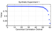
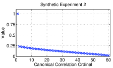
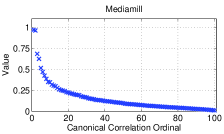
(a)	(b)	(c)

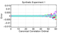
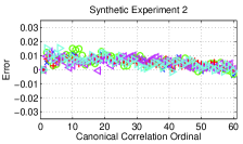
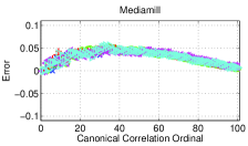
Figure 1: The exact canonical correlations.

(a)	(b)	(c)

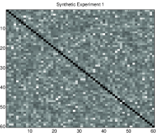
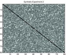
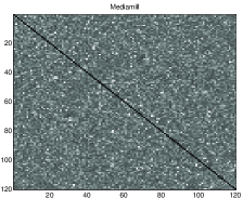
Figure 2: Error in approximation of the canonical correlations.

(a)	(b)	(c)

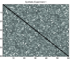
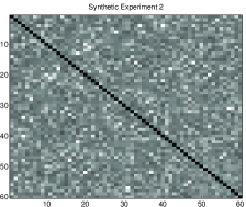
Figure 3: Visualization of the absolute value of the enteries in ${\bm{\mathrm{W}}}^{\textsc{T}}{\bm{\mathrm{A}}}^{\textsc{T}}{\bm{\mathrm{A}}}{\bm{\mathrm{W}}}$ in one of the runs. Color vary between white and black, with black is $1$ and white is $10^{-5}$.

(a)	(b)	(c)

Figure 4: Visualization of the absolute value of the enteries in ${\bm{\mathrm{P}}}^{\textsc{T}}{\bm{\mathrm{B}}}^{\textsc{T}}{\bm{\mathrm{B}}}{\bm{\mathrm{P}}}$ in one of the runs. Color vary between white and black, with black is $1$ and white is $10^{-5}$.

8.1 Synthetic Experiment 1

In this experiment we first draw five random matrices: three matrices ${\bm{\mathrm{G}}},{\bm{\mathrm{W}}},{\bm{\mathrm{Z}}}\in\R^{m\times n}$ with independent entries from the normal distribution, and two matrices ${\bm{\mathrm{X}}},{\bm{\mathrm{Y}}}\in\R^{n\times n}$ with independent entries from the uniform distribution on $[0,1]$. We now set ${\bm{\mathrm{A}}}={\bm{\mathrm{G}}}{\bm{\mathrm{X}}}+0.1\cdot{\bm{\mathrm{W}}}$ and ${\bm{\mathrm{B}}}={\bm{\mathrm{G}}}{\bm{\mathrm{Y}}}+0.1\cdot{\bm{\mathrm{Z}}}$. We use the sizes $m=120,000$ and $n=60$. Conceptually, we first take a random basis (the columns of ${\bm{\mathrm{G}}}$), and linearly transform it in two different ways (by multiplying by ${\bm{\mathrm{X}}}$ and ${\bm{\mathrm{Y}}}$). The transformation does not change the space spanned by the bases. We now add to each base some random noise ($0.1\cdot{\bm{\mathrm{W}}}$ and $0.1\cdot{\bm{\mathrm{Z}}}$). Since both ${\bm{\mathrm{A}}}$ and ${\bm{\mathrm{B}}}$ essentially span the same column space, only polluted by different noise, we expect $({\bm{\mathrm{A}}},{\bm{\mathrm{B}}})$ to have mostly large canonical correlations (close to $1$), but also a few small ones. Indeed, Figure 4(a), which plots the canonical correlations of this pair of matrices, confirms our hypothesis.

Figure 4(a) shows the (signed) error in approximating the canonical correlations, in five different runs. The actual error is always an order of magnitude smaller than the input $\epsilon$; the maximum absolute error is only $0.011$. For large canonical correlations the error is much smaller, and the approximated value is very accurate. For smaller correlations, the error starts to get larger, but it is still an order of magnitude smaller than the actual value for the smallest correlation.

Next, we checked whether ${\bm{\mathrm{A}}}{\bm{\mathrm{W}}}$ and ${\bm{\mathrm{B}}}{\bm{\mathrm{P}}}$ are close to having orthogonal columns, where ${\bm{\mathrm{W}}}$ and ${\bm{\mathrm{P}}}$ contain the canonical weights returned by the proposed algorithm. Figure 4(a) visualizes the entries of ${\bm{\mathrm{W}}}^{\textsc{T}}{\bm{\mathrm{A}}}^{\textsc{T}}{\bm{\mathrm{A}}}{\bm{\mathrm{W}}}$ and figure 4(a) visualizes the entries of ${\bm{\mathrm{P}}}^{\textsc{T}}{\bm{\mathrm{B}}}^{\textsc{T}}{\bm{\mathrm{B}}}{\bm{\mathrm{P}}}$ in one of the runs. We see that the diagonal is dominant, and close to 1, and the off diagonal entries are small (but not tiny). The maximum condition number of ${\bm{\mathrm{A}}}{\bm{\mathrm{W}}}$ and ${\bm{\mathrm{B}}}{\bm{\mathrm{P}}}$ we got in the five different runs was $1.08$, indicating the columns are indeed close to be orthogonal.

As for the running time, the proposed algorithm takes about 55% less time than Björck and Golub’s algorithm ($0.915$ seconds vs. $2.04$ seconds).

8.2 Synthetic Experiment 2

In this experiment we first draw three random matrices. The first matrix ${\bm{\mathrm{X}}}\in\R^{m\times n}$ has independent entries from the normal distribution. The second matrix ${\bm{\mathrm{Y}}}\in\R^{m\times k}$ has independent entries which take value $\pm 1$ with equal probability. The third matrix ${\bm{\mathrm{Z}}}\in\R^{k\times n}$ has independent entries from the uniform distribution on $[0,1]$. We now set ${\bm{\mathrm{A}}}={\bm{\mathrm{X}}}+0.1\cdot{\bm{\mathrm{Y}}}\cdot\left({\bm{1}}_{k\times n}+{\bm{\mathrm{Z}}}\right)$ and ${\bm{\mathrm{B}}}={\bm{\mathrm{Y}}}$, where ${\bm{1}}_{k\times n}$ is the $k\times n$ all-ones matrix. We use the sizes $m=80,000$, $n=80$ and $k=60$. Here we basically have noise (${\bm{\mathrm{B}}}$) and a matrix polluted with that noise (${\bm{\mathrm{A}}}$). So there is some correlation, but really the two subspaces are different; there is one large correlation (almost $1$) and all the rest are small (Figure 4(b)).

Figure 4(b) shows the (signed) error in approximating the correlations, in five different runs. The actual error is an order of magnitude smaller than the target $\epsilon$; the maximum absolute error is only $0.02$. Again, for the largest canonical correlation (which is close to $1$) the result is very accurate, with tiny errors. For the other correlations it is larger. For tiny correlations the error is about of the same magnitude as the actual value. Interestingly, we observe a bias towards over-estimating the correlations.

Next, we checked whether ${\bm{\mathrm{A}}}{\bm{\mathrm{W}}}$ and ${\bm{\mathrm{B}}}{\bm{\mathrm{P}}}$ are close to having orthogonal columns, where ${\bm{\mathrm{W}}}$ and ${\bm{\mathrm{P}}}$ contain the canonical weights returned by the proposed algorithm. Figure 4(b) visualizes the entries of ${\bm{\mathrm{W}}}^{\textsc{T}}{\bm{\mathrm{A}}}^{\textsc{T}}{\bm{\mathrm{A}}}{\bm{\mathrm{W}}}$ and figure 4(b) visualizes the entries of ${\bm{\mathrm{P}}}^{\textsc{T}}{\bm{\mathrm{B}}}^{\textsc{T}}{\bm{\mathrm{B}}}{\bm{\mathrm{P}}}$ in one of the runs. We see that the diagonal is dominant, and close to 1, and the off diagonal entries are small (but not tiny). The maximum condition number of ${\bm{\mathrm{A}}}{\bm{\mathrm{W}}}$ and ${\bm{\mathrm{B}}}{\bm{\mathrm{P}}}$ we got in the five different runs was $1.08$, indicating the columns are indeed close to be orthogonal.

As for the running time, the proposed algorithm takes about 40% less time than Björck and Golub’s algorithm ($1.77$ seconds vs. $1.77$ seconds).

8.3 Real-life dataset: Mediamill

We also tested the proposed algorithm on the annotated video dataset from the Mediamill Challenge [27]. Combining the training set and the challenge set, 43907 images are provided, each image is a representative keyframe image of a video shot. The dataset provides 120 features for each image, and the set is annotated with 101 labels. The label matrix is rank-deficient with rank 100. Figure 4(c) shows the exact canonical correlations. We see there is a few high correlations, with very strong decay afterwards.

Figure 4(c) shows the (signed) error in approximating the correlations, in five different runs. The maximum absolute error is rather small (only 0.055). For the large correlations, which are the more interesting ones in this context, the error is much smaller, so we have a relatively high accuracy approximation. Again, there is an interesting bias towards over-estimating the correlations.

Next, we checked whether ${\bm{\mathrm{A}}}{\bm{\mathrm{W}}}$ and ${\bm{\mathrm{B}}}{\bm{\mathrm{P}}}$ are close to having orthogonal columns, where ${\bm{\mathrm{W}}}$ and ${\bm{\mathrm{P}}}$ contain the canonical weights returned by the proposed algorithm. Figure 4(c) visualizes the entries of ${\bm{\mathrm{W}}}^{\textsc{T}}{\bm{\mathrm{A}}}^{\textsc{T}}{\bm{\mathrm{A}}}{\bm{\mathrm{W}}}$ and figure 4(c) visualizes the entries of ${\bm{\mathrm{P}}}^{\textsc{T}}{\bm{\mathrm{B}}}^{\textsc{T}}{\bm{\mathrm{B}}}{\bm{\mathrm{P}}}$ in one of the runs. We see that the diagonal is dominant, and close to 1, and the off diagonal entries are small (but not tiny). The maximum condition number of ${\bm{\mathrm{A}}}{\bm{\mathrm{W}}}$ and ${\bm{\mathrm{B}}}{\bm{\mathrm{P}}}$ we got in the five different runs was $1.23$, which is larger than the previous two examples, but still indicating the columns are not too far from being orthogonal.

As for the running time, the proposed algorithm is considerably faster than Björck and Golub’s algorithm ($0.69$ sec vs. $2.03$ sec).

8.4 Summary

The experiments are not exhaustive, but they do suggest the following. First, it appears that the sampling size bounds are rather loose. The algorithm achieves much better approximation errors. Second, there seems to be a connection between the canonical correlation value and the error: for larger correlations the error is smaller. Our bounds fail to capture these phenomena. Finally, the experiments show that the proposed is faster than Björck and Golub’s algorithm in practice on both synthetic and real-life datasets, even if they are fairly small. We expect the difference to be much larger on big datasets.

9 Conclusions

We proved that dimensionality reduction via Randomized Fast Unitary Transforms leads to faster algorithms for Canonical Correlation Analysis, beating the seminal SVD-based algorithm of Björck and Golub.

The proposed algorithm builds upon a family of similar algorithms which, in recent years, led to similar running time improvements for other classical linear algebraic and machine learning problems: (i) Least-squares regression [25, 6, 14, 3]; (ii) approximate PCA (via low-rank matrix approximation) [17]; (iii) matrix multiplication [26]; (v) K-means clustering [7]; (vi) support vector machines [24].

References

- [1] N. Ailon and B. Chazelle. Approximate nearest neighbors and the fast johnson-lindenstrauss transform. In Proceedings of the Symposium on Theory of Computing (STOC), pages 557–563, 2006.
- [2] N. Ailon and E. Liberty. Fast dimension reduction using Rademacher series on dual BCH codes. In Proceedings of the ACM-SIAM Symposium on Discrete Algorithms (SODA), 2008.
- [3] H. Avron, P. Maymounkov, and S. Toledo. Blendenpik: Supercharging LAPACK’s least-squares solver. SIAM Journal on Scientific Computing, 32(3):1217–1236, 2010.
- [4] Z. Bar-Yossef, T. S. Jayram, R. Kumar, and D. Sivakumar. An information statistics approach to data stream and communication complexity. J. Comput. Syst. Sci., 68(4):702–732, 2004.
- [5] A. Björck and G.H. Golub. Numerical methods for computing angles between linear subspaces. Mathematics of Computation, 27(123):579–594, 1973.
- [6] C. Boutsidis and P. Drineas. Random projections for the nonnegative least-squares problem. Linear Algebra and its Applications, 431(5-7):760–771, 2009.
- [7] C. Boutsidis, A. Zouzias, and P. Drineas. Random projections for -means clustering. In Neural Information Processing Systems (NIPS), 2010.
- [8] A. Chattopadhyay and T. Pitassi. The story of set disjointness. SIGACT News, 41(3):59–85, 2010.
- [9] K. Chaudhuri, S. M. Kakade, K. Livescu, and K. Sridharan. Multi-view clustering via canonical correlation analysis. In International Conference in Machine Learning (ICML), pages 129–136, 2009.
- [10] K. L. Clarkson and D. P. Woodruff. Low Rank Approximation and Regression in Input Sparsity Time. In Proceedings of the Symposium on Theory of Computing (STOC), 2013.
- [11] P. Dhillon, J. Rodu, D. Foster, and L. Ungar. Two step CCA: A new spectral method for estimating vector models of words. In Proceedings of the 29th International Conference on Machine Learning, ICML’12, 2012.
- [12] P. S. Dhillon, D. Foster, and L. Ungar. Multi-view learning of word embeddings via CCA. In Neural Information Processing Systems (NIPS), 2011.
- [13] P. Drineas, M. Magdon-Ismail, M. W. Mahoney, and D. P. Woodruff. Fast approximation of matrix coherence and statistical leverage. In International Conference in Machine Learning (ICML), 2012.
- [14] P. Drineas, M.W. Mahoney, S. Muthukrishnan, and T. Sarlós. Faster least squares approximation. Numerische Mathematik, 117(2):217–249, 2011.
- [15] S. Eisenstat and I. Ipsen. Relative perturbation techniques for singular value problems. SIAM Journal on Numerical Analysis, 32:1972–1988, 1995.
- [16] G.H. Golub and H. Zha. The canonical correlations of matrix pairs and their numerical computation. IMA Volumes in Mathematics and its Applications, 69:27–27, 1995.
- [17] N. Halko, P.G. Martinsson, and J.A. Tropp. Finding structure with randomness: Probabilistic algorithms for constructing approximate matrix decompositions. SIAM Review, 53(2):217–288, 2011.
- [18] R. A. Horn and C. R. Johnson. Matrix Analysis. Cambridge University Press, 1985.
- [19] H. Hotelling. Relations between two sets of variates. Biometrika, 28(3/4):321–377, 1936.
- [20] I. Ipsen and T.. Wentworth. The effect of coherence on sampling from matrices with orthonormal columns, and preconditioned least squares problems. Arxiv preprint arXiv:1203.4809, 2012.
- [21] T.-K. Kim, J. Kittler, and R. Cipolla. Discriminative learning and recognition of image set classes using canonical correlations. IEEE Trans. Pattern Anal. Mach. Intell., 29(6):1005–1018, 2007.
- [22] E. Kushilevitz and N. Nisan. Communication complexity. Cambridge University Press, New York, NY, USA, 1997.
- [23] X. Meng and M. W. Mahoney. Low-distortion Subspace Embeddings in Input-sparsity Time and Applications to Robust Linear Regression. In Proceedings of the Symposium on Theory of Computing (STOC), 2013.
- [24] S. Paul, C. Boutsidis, M. Magdon-Ismail, and P. Drineas. Random projections for support vector machines. In International Conference on Artificial Intelligence and Statistics (AISTATS), 2013.
- [25] V. Rokhlin and M. Tygert. A fast randomized algorithm for overdetermined linear least-squares regression. Proceedings of the National Academy of Sciences, 105(36):13212, 2008.
- [26] T. Sarlós. Improved approximation algorithms for large matrices via random projections. In Proceedings of the Symposium on Foundations of Computer Science (FOCS), 2006.
- [27] C. G. M. Snoek, M. Worring, J. C. van Gemert, J. M. Geusebroek, and A. W. M. Smeulders. The challenge problem for automated detection of 101 semantic concepts in multimedia. In Proceedings of the ACM International Conference on Multimedia, pages 421–430, 2006.
- [28] Y. Su, Y. Fu, X. Gao, and Q. Tian. Discriminant learning through multiple principal angles for visual recognition. IEEE Transactions on Image Processing, 21(3):1381 –1390, March 2012.
- [29] L. Sun, B. Ceran, and J. Ye. A scalable two-stage approach for a class of dimensionality reduction techniques. In ACM SIGKDD Conference on Knowledge Discovery and Data Mining (KDD), pages 313–322, 2010.
- [30] L. Sun, S. Ji, and J. Ye. A least squares formulation for canonical correlation analysis. In International Conference in Machine Learning (ICML), pages 1024–1031, 2008.
- [31] A. Talwalkar and A. Rostamizadeh. Matrix coherence and the Nyström method. In UAI, pages 572–579, 2010.
- [32] J. A. Tropp. Improved analysis of the subsampled randomized Hadamard transform. Adv. Adapt. Data Anal., special issue, “Sparse Representation of Data and Images”, 2011.
- [33] A. C.-C. Yao. Some complexity questions related to distributive computing (Preliminary Report). In Proceedings of the Symposium on Theory of Computing (STOC), pages 209–213, 1979.