Graph Expansion Analysis for Communication Costs of Fast Rectangular Matrix Multiplication

Abstract

Graph expansion analysis of computational DAGs is useful for obtaining communication cost lower bounds where previous methods, such as geometric embedding, are not applicable. This has recently been demonstrated for Strassen’s and Strassen-like fast square matrix multiplication algorithms. Here we extend the expansion analysis approach to fast algorithms for rectangular matrix multiplication, obtaining a new class of communication cost lower bounds. These apply, for example to the algorithms of Bini et al. (1979) and the algorithms of Hopcroft and Kerr (1971). Some of our bounds are proved to be optimal.

1 Introduction

The time cost of an algorithm, sequential or parallel, depends not only on how many computational operations it executes but also on how much data it moves. In fact, the cost of data movement, or communication, is often much more expensive than the cost of computation. Architectural trends predict that computation cost will continue to decrease exponentially faster than communication cost, leading to ever more algorithms that are dominated by the communication costs. Thus, in order to minimize running times, algorithms should be designed with careful consideration of their communication costs. To that end, we discuss asymptotic costs of algorithms in terms of both number of computations performed (flops in the case of numerical algorithms) and units of communication: words moved.

For a sequential algorithm, we determine the communication cost incurred on a simple machine model which consists of two levels of memory hierarchy, as described in Section 1.3. In many cases, naïve implementations of algorithms incur communication costs much higher than necessary; reformulating the algorithm to performing the same arithmetic in a different order can drastically decrease the communication costs and therefore the total running time. In order to determine the possible improvements and identify whether an algorithm is optimal with respect to communication costs, one seeks communication lower bounds.

Hong and Kung [17] were the first to prove communication lower bounds for matrix multiplication algorithms. They show that on a two-level machine model, any algorithm which performs the $\Theta(n^{3})$ flops of classical matrix multiplication must move at least $\Omega(n^{3}/\sqrt{M})$ words between fast and slow memory, where $M$ is the number of words that can fit simultaneously in fast memory. Irony, Toledo, and Tiskin [22] generalized their classical matrix multiplication result to a distributed-memory parallel machine model using a geometric embedding argument. Ballard, Demmel, Holtz and Schwartz [4] showed this proof technique is applicable to a more general set of computations, including one-sided matrix factorizations such as LU, Cholesky, and QR and two-sided matrix factorizations which are used in eigenvalue and singular value computations, most of which perform $\Theta(n^{3})$ computations in the dense matrix case. Many of these bounds on $\Theta(n^{3})$ algorithms have been shown to be optimal.

However, the geometric embedding approach does not seem to apply to computations which do not map to a simple geometric computation space. In the case of classical matrix multiplication and other $O(n^{3})$ algorithms, the computation corresponds to a three-dimensional lattice. In particular, the geometric embedding approach does not readily apply to Strassen’s algorithm for matrix multiplication that requires $O(n^{\log_{2}7})$ flops. Instead, Ballard, Demmel, Holtz, and Schwartz [5] show that a different proof technique based on analysis of the expansion properties of the computational directed acyclic graph (CDAG) can be used to obtain communication lower bounds for both sequential and parallel models for these algorithms. The proof technique can also be used to bound how well the corresponding parallel algorithms can strongly-scale [2]. We use this same approach here to prove bounds on fast rectangular matrix multiplication algorithms, which introduce some extra technical challenges.

1.1 Expansion and communication

The CDAG of a recursive algorithm has a recursive structure, and thus its expansion can be analyzed combinatorially (similarly to what is done for expander graphs in [30, 1, 26]) or by spectral analysis (in the spirit of what was done for the Zig-Zag expanders [31]). Analyzing the CDAG for communication cost bounds was first suggested by Hong and Kung [17]. They use the red-blue pebble game to obtain tight lower bounds on the communication costs of many algorithms, including classical $\Theta(n^{3})$ matrix multiplication, matrix-vector multiplication, and FFT. Their proof is obtained by considering dominator sets of the CDAG.

Other papers study connections between bounded space computation and combinatorial expansion-related properties of the corresponding CDAG (see e.g., [32, 9, 8] and references therein). The study of expansion properties of a CDAG was also suggested as one of the main motivations of Lev and Valiant [28] in their work on superconcentrators and lower bounds on the arithmetic complexity of various problems.

1.2 Fast rectangular matrix multiplication

Following Strassen’s algorithm for fast multiplication of square matrices [33], the arithmetic complexity of multiplying rectangular matrices has been extensively studied (see [19, 11, 13, 29, 20, 21, 14] and further details in [12]). When there is an algorithm for multiplying an $m\times n$ matrix $A$ with an $n\times p$ matrix $B$ to obtain an $m\times p$ matrix $C$ using only $q$ scalar multiplications, we use the notation $\langle m,n,p\rangle=q$. The above studies try to minimize the number of multiplications $q$ (as a function of $m,n,$ and $p$). A particular focus of interest is maximizing $\alpha$ so that $\langle n,n,n^{\alpha}\rangle=O(n^{2}\log n)$ namely maximizing the size of a rectangular matrix, so that it can be multiplied (from right) with a square matrix, in time which is only slightly more than what is needed to read the input. Recall that $\langle m,n,p\rangle=\langle n,p,m\rangle=\langle p,m,n\rangle=\langle m,p,n\rangle=\langle p,n,m\rangle=\langle n,m,p\rangle$ for all $m,n,p$ [18].

Rectangular matrix multiplication is used in many algorithms, for solving problems in linear algebra, in combinatorial optimization, and other areas. Utilizing fast algorithms for rectangular matrix multiplication has proved to be quite useful for improving the complexity of solving many of those problems (a very partial list includes [16, 25, 7, 36, 27, 34, 35, 23, 24]).

1.3 Communication model

We model communication costs on a sequential machine as follows. Assume the machine has a fast memory of size $M$ words and a slow memory of infinite size. Further assume that computation can be performed only on data stored in the fast memory. On a real computer, this model may have several interpretations and may be applied to anywhere in the memory hierarchy. For example the slow memory might be the hard drive and the fast memory the DRAM; or the slow memory might be the DRAM and the fast memory the cache.

The goal is to minimize the number of words $W$ transferred between fast and slow memory, which we call the communication cost of an algorithm. Note that we minimize with respect to an algorithm, not with respect to a problem, and so the only optimization allowed is re-ordering the computation in a way that is consistent with the CDAG of the algorithm. The sequential communication cost is closely related to communication costs in the various parallel models. We discuss this relationship briefly in Section 6.

1.4 The communication costs of rectangular matrix multiplication

The communication costs lower bounds of rectangular matrix multiplication algorithms are determined by properties of the underlying CDAGs. Consider $\langle m^{t},n^{t},p^{t}\rangle=q^{t}$ matrix multiplication that is generated from $t$ tensor powers of $\langle m,n,p\rangle=q$. Denote the former by the algorithm and the latter by the base case, and consider their CDAGs. They both consist of four parts: the encoding graphs of $A$ and $B$, the scalar multiplications, and the decoding graph of $C$. The encoding graphs correspond to computing linear combinations of entries of $A$ or $B$, and the decoding graph to computing linear combinations of the scalar products. See Figure 1 in Section 4 for a diagram of the algorithm CDAG, and Figure 2 in Section 5 for an example of a base-case CDAG. Let us state the communication cost lower bounds of the two main cases.

Theorem 1

Let $\langle m^{t},n^{t},p^{t}\rangle=q^{t}$ be the algorithm obtained from a base case $\langle m,n,p\rangle=q$. If the decoding graph of the base case is connected, then the communication cost lower bound is

$$W=\Omega\left(\frac{q^{t}}{M^{\log_{mp}q-1}}\right).$$

Further, in the case that $n\leq m$ and $n\leq p$ this bound is tight.

Note that in the case $m=n=p$, this result reproduces the lower bound for Strassen-like square matrix multiplication algorithms in [5]. In this case, for $\omega_{0}=\log_{n}q$, we obtain $W=\Omega\left(\frac{(n^{t})^{\omega_{0}}}{M^{\omega_{0}/2-1}}\right)$.

Theorem 2

Let $\langle m^{t},n^{t},p^{t}\rangle=q^{t}$ be the algorithm obtained from a base case $\langle m,n,p\rangle=q$. If an encoding graph of the base case is connected and has no multiply-copied inputs, then

$$W=\Omega\left(\frac{q^{t}}{t^{\log_{N}q}M^{\log_{N}q-1}}\right),$$

where $N=mn$ or $N=np$ is the size of the input to the encoding graph. Further, this bound is tight if $N=\max\{mn,np,mp\}$, up to a factor of $t^{\log_{N}q}$, which is a polylogarithmic factor in the input size.

We also treat the cases of disconnected encoding and decoding graphs and obtain similar bounds with restrictions on the fast memory size $M$. See Corollaries 13 and 14 in Section 4.

These theorems and corollaries apply in particular to the algorithms of Bini et al. [11] and Hopcroft and Kerr [19], which we detail in Section 5.

1.5 Paper organization

In Section 2 we state some preliminary facts about the computational graph and edge expansion. Section 3 explains the connection between communication cost and edge expansion. The proofs of the lower bound theorems stated in Section 1.4, as well as some extensions, appear in Section 4. In Section 5 we apply our new lower bounds to two example algorithms: Bini’s algorithm and the Hopcroft-Kerr algorithm. Appendix A gives further details of Bini’s algorithm and the Hopcroft-Kerr algorithm.

2 Preliminaries

2.1 The Computational Graph

For a given algorithm, we consider the CDAG $G=(V,E)$, where there is a vertex for each arithmetic operation (AO) performed, and for every input element. $G$ contains a directed edge $(u,v)$, if the output operand of the AO corresponding to $u$ (or the input element corresponding to $u$), is an input operand to the AO corresponding to $v$. The in-degree of any vertex of $G$ is, therefore, at most 2 (as the arithmetic operations are binary). The out-degree is, in general, unbounded, i.e., it may be a function of $|V|$.

2.1.1 The relaxed computational graph.

For a given recursive algorithm, the relaxed computational graph is almost identical to the computational DAG with the following change: when a vertex corresponds to re-using data across recursive levels, we replace it with several connected “copy vertices,” each of which exists in one recursive level. While the CDAG of a recursive algorithm may have vertices of degree that depend on $|V|$, this relaxed CDAG has constant bounded degree. We use the relaxed graph to handle such cases in Section 4.2.

2.1.2 Multiply-copied vertices.

We say that a base-case encoding subgraph has no multiply-copied vertices if each input vertex appears at most once as an output vertex. An output vertex $v$ is copied from an input vertex if the in-degree of $v$ is exactly one. See, for example, Figure 2. The vertex $a_{11}$ is copied to the third output of $Enc_{1}A$ but is not copied to any other outputs. Since all other inputs are also copied at most once, there are no multiply-copied vertices in Figure 2.

This condition is necessary for the degree of the entire algorithm’s encoding subgraph to be at most logarithmic in the size of the input. We are not aware of any fast matrix multiplication algorithm that has multiply-copied vertices, although the recursive formulation of classical matrix multiplication does.

2.2 Edge expansion

The edge expansion $h(G)$ of a $d$-regular undirected graph $G=(V,E)$ is:

$$h(G)\equiv\min_{U\subseteq V,|U|\leq|V|/2}\frac{|E(U,V\setminus U)|}{d\cdot|U|}$$

where $E(A,B)\equiv E_{G}(A,B)$ is the set of edges connecting the vertex sets $A$ and $B$. We omit the subscript $G$ when the context makes it clear. Treating a CDAG as undirected simplifies the analysis and does not affect the asymptotic communication cost. For many graphs, small sets expand more than larger sets. Let $h_{s}(G)$ denote the edge expansion for sets of size at most $s$ in $G$:

$$h_{s}(G)\equiv\min_{U\subseteq V,|U|\leq s}\frac{|E(U,V\setminus U)|}{d\cdot|U|}~{}.$$

Note that CDAGs are typically not regular. If a graph $G=(V,E)$ is not regular but has a bounded maximal degree $d$, then we can add ($<d$) loops to vertices of degree $<d$, obtaining a regular graph $G^{\prime}$. We use the convention that a loop adds 1 to the degree of a vertex. Note that for any $S\subseteq V$, we have $|E_{G}(S,V\setminus S)|=|E_{G^{\prime}}(S,V\setminus S)|$, as none of the added loops contributes to the edge expansion of $G^{\prime}$.

2.3 Matching sequential algorithm

In many cases, the communication cost lower bounds are matched by the naïve recursive algorithm. The cost of the recursive algorithm applied to $\langle m^{t},n^{t},p^{t}\rangle=q^{t}$, taking $N^{*}=\max\{mn,np,mp\}$ is

$$W(t)=\left\{\begin{array}[]{ll}q\cdot W(t-1)+\Theta\left((N^{*})^{t-1}\right)&\textrm{if }(N^{*})^{t}>M/3\\ 3(N^{*})^{t}&\textrm{otherwise}\end{array}\right.,$$

since the algorithm does not communicate once the three matrices fit into fast memory. The solution to this recurrence is given by

$$W=\Theta\left(\frac{q^{t}}{M^{\log_{N^{*}}q-1}}\right).$$

3 Communication Cost and Edge Expansion

In this section we recall the partition argument and how to combine it with edge expansion analysis to obtain communication cost lower bounds. This follows our approach in [5, 2]. A similar partition argument previously appeared in [17, 22, 4], where other techniques (geometric or combinatorial) are used to connect the number of flops to the amount of data in a segment.

3.1 The partition argument

Let $M$ be the size of the fast memory. Let $O$ be any total ordering of the vertices that respects the partial ordering of the CDAG $G$. This total ordering can be thought of as the actual order in which the computations are performed. Let ${\cal P}$ be any partition of $V$ into segments $S_{1},S_{2},...$, so that a segment $S_{i}\in{\cal P}$ is a subset of the vertices that are contiguous in the total ordering $O$.

Let $R_{S}$ and $W_{S}$ be the set of read and write operands, respectively. Namely, $R_{S}$ is the set of vertices outside $S$ that have an edge going into $S$, and $W_{S}$ is the set of vertices in $S$ that have an edge going outside of $S$. Then the total communication costs due to reads of AOs in $S$ is at least $|R_{S}|-M$, as at most $M$ of the needed $|R_{S}|$ operands are already in fast memory when the execution of the segment’s AOs starts. Similarly, $S$ causes at least $|W_{S}|-M$ actual write operations, as at most $M$ of the operands needed by other segments are left in the fast memory when the execution of the segment’s AOs ends. The total communication cost is therefore bounded below by

$$W \geq \min_{{\cal P}}\sum_{S\in{\cal P}}\left(|R_{S}|+|W_{S}|-2M\right)~{}.$$ (1)

3.2 Edge expansion and communication cost

Consider a segment $S$ and its read and write operands $R_{S}$ and $W_{S}$.

Proposition 3

If the graph $G$ containing $S$ has $h_{s}(G)$ edge expansion for sets of size $s=|S|$, maximum (constant) degree $d$, and at least $2|S|$ vertices, then $|R_{S}|+|W_{S}|\geq\frac{1}{2}\cdot h_{s}(G)\cdot|S|$ .

Proof   We have $|E(S,V\setminus S)|\geq h_{s}(G)\cdot d\cdot|S|$. Either (at least) half of the edges $E(S,V\setminus S)$ touch $R_{S}$ or half of them touch $W_{S}$. As every vertex is of degree $d$, we have $|R_{S}|+|W_{S}|\geq\max\{|R_{S}|,|W_{S}|\}\geq\frac{1}{d}\cdot\frac{1}{2}\cdot|E(S,V\setminus S)|\geq h_{s}(G)\cdot|S|/2$.  

Combining this with (1) and choosing to partition $V$ into $|V|/s$ segments of equal size $s$, we obtain: $W\geq\max_{s}\frac{|V|}{s}\cdot\left(\frac{h_{s}(G)\cdot s}{2}-2M\right)$. Choosing the minimal $s$ so that

$$\frac{h_{s}(G)\cdot s}{2}\geq 3M$$ (2)

we obtain

$$W \geq \frac{|V|}{s}\cdot M~{}.$$ (3)

In some cases, as in fast square and rectangular matrix multiplication, the computational graph $G$ does not fit this analysis: it may not be regular, it may have vertices of unbounded degree, or its edge expansion may be hard to analyze. In such cases, we may then consider some subgraph $G^{\prime}$ of $G$ instead to obtain a lower bound on the communication cost. The natural subgraph to select in fast (square and rectangular) matrix multiplication algorithms is the decoding graph or one of the two encoding graphs.

4 Expansion Properties of Fast Rectangular Matrix Multiplication Algorithms

There are several technical challenges that we deal with in the rectangular case, on top of the analysis in [5] (where we deal with the difference between addition and multiplication vertices in the recursive construction of the CDAG). These additional challenges arise from the differences between the CDAG of rectangular algorithms, such as Bini’s algorithm and the Hopcroft-Kerr algorithm on the one hand, and of Strassen’s algorithm on the other hand. The three subgraphs, two encoding and one decoding, are of the same size in Strassen’s and of unequal size in rectangular algorithms. The largest expansion guarantee is given by the subgraph corresponding to the largest of the three matrices. One consequence is that it is necessary to consider the case of unbounded degree vertices that may appear in the encoding subgraphs. Additionally, in some cases the encoding or decoding graphs consist of several disconnected components.

4.1 The computational graph for $\langle m^{t},n^{t},p^{t}\rangle=q^{t}$

Consider the computational graph $H_{t}$ associated with multiplying a matrix $A$ of dimension $m^{t}\times n^{t}$ by a matrix $B$ of dimension $n^{t}\times p^{t}$. Denote by $Enc_{t}A$ the part of $H_{t}$ that corresponds to the encoding of matrix $A$. Similarly, $Enc_{t}B$, and $Dec_{t}C$ correspond to the parts of $H_{t}$ that compute the encoding of $B$ and the decoding of $C$, respectively (see Figure 1).

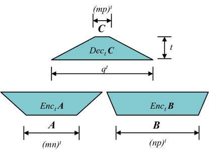
Figure 1: Computational graph for $\langle m^{t},n^{t},p^{t}\rangle=q^{t}$ rectangular matrix multiplication generated from $t$ recursive levels with base graph given by $\langle m,n,p\rangle=q$. In this figure $m<p<n$.

4.1.1 A top-down construction of the computational graph.

We next construct the computational graph $H_{i+1}$ by constructing $Dec_{i+1}C$ from $Dec_{i}C$ and $Dec_{1}C$ and similarly constructing $Enc_{i+1}A$ and $Enc_{i+1}B$, then composing the three parts together.

1. Duplicate $Dec_{1}C$ $q^{i}$ times.

2. Duplicate $Dec_{i}C$ $mp$ times.

3. Identify the $mp\cdot q^{i}$ output vertices of the copies of $Dec_{1}C$ with the $mp\cdot q^{i}$ input vertices of the copies of $Dec_{i}C$:

   • Recall that each $Dec_{1}C$ has $mp$ output vertices.

   • The first output vertex of the $q^{i}$ $Dec_{1}C$ graphs are identified with the $q^{i}$ input vertices of the first copy of $Dec_{i}C$.

   • The second output vertex of the $q^{i}$ $Dec_{1}C$ graphs are identified with the $q^{i}$ input vertices of the second copy of $Dec_{i}C$. And so on.

   • We make sure that the $j$th input vertex of a copy of $Dec_{i}C$ is identified with an output vertex of the $j$th copy of $Dec_{1}C$.

4. We similarly obtain $Enc_{i+1}A$ from $Enc_{i}A$ and $Enc_{1}A$,

5. and $Enc_{i+1}B$ from $Enc_{i}B$ and $Enc_{1}B$.

6. For every $i$, $H_{i}$ is obtained by connecting edges from the $j$th output vertices of $Enc_{i}A$ and $Enc_{i}B$ to the $j$th input vertex of $Dec_{i}C$.

This completes the construction. Let us note some properties of this graphs.

As all out-degrees are at most $mp$ and all in degree are at most 2 we have:

Proposition 4

All vertices of $Dec_{t}C$ are of degree at most $mp+2$, as long as $n>1$ (that is, as long as the base case is not an outer product).

Proof   If the set of input vertices of $Dec_{1}C$ and the set of its output vertices are disjoint, then the proposition follows.. Assume (towards contradiction) that the base graph $Dec_{1}C$ has an input vertex which is also an output vertex. An output vertex represents the inner product of two $n$-vectors, i.e., the corresponding row-vector of $A$ and column vector of $B$. The corresponding bilinear polynomial is irreducible. This is a contradiction, since $n>1$ an input vertex represents the multiplication of a (weighted) sum of elements of $A$ with a (weighted) sum of elements of $B$.  

Note, however, that $Enc_{1}A$ and $Enc_{1}B$ may have vertices which are both inputs and outputs, therefore $Enc_{t}A$ and $Enc_{t}B$ may have vertices of out-degree which is a function of $t$. In [5, 2], it was enough to analyze $Dec_{t}C$ and lose only a constant factor in the lower bound. However in several rectangular matrix multiplication algorithms, it is necessary to consider the encoding graphs as well, since they may provide a better expansion than the decoding graph.

Lemma 5

If $Dec_{1}C$ is connected, then the edge expansion of $Dec_{t}C$ is

$$h(Dec_{t}C)=\Omega\left(\left(\frac{mp}{q}\right)^{t}\right).$$

Proof   The proof follows that of Lemma 4.9 in [5] adapting the corresponding parameters. We provide it here for completeness. Let $G_{t}=(V,E)$ be $Dec_{t}C$, and let $S\subseteq V,|S|\leq|V|/2$. We next show that $|E(S,V\setminus S)|\geq c\cdot d\cdot|S|\cdot\left(\frac{mp}{q}\right)^{t}$, where $c$ is some universal constant, and $d$ is the constant degree of $Dec_{t}C$ (after adding loops to make it regular).

The proof works as follows. Recall that $G_{t}$ is a layered graph (with layers corresponding to recursion steps), so all edges (excluding loops) connect between consecutive levels of vertices. We argue (in Proposition 9) that each level of $G_{t}$ contains about the same fraction of $S$ vertices, or else we have many edges leaving $S$. We also observe (in Fact 10) that such homogeneity (of a fraction of $S$ vertices) does not hold between distinct parts of the lowest level, or, again, we have many edges leaving $S$. We then show that the homogeneity between levels, combined with the heterogeneity of the lowest level, guarantees that there are many edges leaving $S$.

Let $l_{i}$ be the $i$th level of vertices of $G_{t}$, so $(mp)^{t}=|l_{1}|<|l_{2}|<\cdots<|l_{i}|=(mp)^{t-i+1}q^{i-1}<\cdots<|l_{t+1}|=q^{t}$. Let $S_{i}\equiv S\cap l_{i}$. Let $\sigma=\frac{|S|}{|V|}$ be the fractional size of $S$ and $\sigma_{i}=\frac{|S_{i}|}{|l_{i}|}$ be the fractional size of $S$ at level $i$. Let $\delta_{i}=\sigma_{i}-\sigma_{i+1}$. Due to averaging, we observe the following:

Fact 6

There exist $i$ and $i^{\prime}$ such that $\sigma_{i}\leq\sigma\leq\sigma_{i^{\prime}}$.

Fact 7

$$|V| = \sum_{i=1}^{t+1}|l_{i}|=\sum_{i=1}^{t+1}|l_{t+1}|\cdot\left(\frac{mp}{q}\right)^{i}$$

$$= |l_{t+1}|\cdot\left(1-\left(\frac{mp}{q}\right)^{t+2}\right)\cdot\frac{q}{q-mp}$$

$$= \left(\frac{mp}{q}\right)^{t}\cdot|l_{1}|\cdot\left(1-\left(\frac{mp}{q}\right)^{t+2}\right)\cdot\frac{q}{q-mp}.$$

so $\frac{q-mp}{q}\leq\frac{|l_{t+1}|}{|V|}\leq\frac{q-mp}{q}\cdot\frac{1}{1-\left(\frac{mp}{q}\right)^{t+2}}$, and $\frac{q-mp}{q}\cdot\left(\frac{mp}{q}\right)^{t}\leq\frac{|l_{1}|}{|V|}\leq\frac{q-mp}{q}\cdot\left(\frac{mp}{q}\right)^{t}\cdot\frac{1}{1-\left(\frac{mp}{q}\right)^{t+2}}.$

Proposition 8

There exists $c^{\prime}=c^{\prime}(G_{1})$ so that $|E(S,V\setminus S)\cap E(l_{i},l_{i+1})|\geq c^{\prime}\cdot d\cdot|\delta_{i}|\cdot|l_{i}|$.

Proof of Proposition 8   Let $G^{\prime}$ be a $G_{1}$ component connecting $l_{i}$ with $l_{i+1}$ (so it has $mp$ vertices in $l_{i}$ and $q$ in $l_{i+1}$). $G^{\prime}$ has no edges in $E(S,V\setminus S)$ if all or none of its vertices are in $S$. Otherwise, as $G^{\prime}$ is connected, it contributes at least one edge to $E(S,V\setminus S)$. The number of such $G_{1}$ components with all their vertices in $S$ is at most $\min\{\sigma_{i},\sigma_{i+1}\}\cdot\frac{|l_{i}|}{mp}$. Therefore, there are at least $|\sigma_{i}-\sigma_{i+1}|\cdot\frac{|l_{i}|}{mp}$ $G_{1}$ components with at least one vertex in $S$ and one vertex that is not.  

Proposition 9 (Homogeneity between levels)

If there exists $i$ so that $\frac{|\sigma-\sigma_{i}|}{\sigma}\geq\frac{1}{10}$, then

$$|E(S,V\setminus S)|\geq c\cdot d\cdot|S|\cdot\left(\frac{mp}{q}\right)^{t}$$

where $c>0$ is some constant depending on $G_{1}$ only.

Proof of Proposition 9   Assume that there exists $j$ so that $\frac{|\sigma-\sigma_{j}|}{\sigma}\geq\frac{1}{10}$. By Proposition 8, we have

$$|E(S,V\setminus S)| \geq \sum_{i\in[t]}|E(S,V\setminus S)\cap E(l_{i},l_{i+1})|$$

$$\geq \sum_{i\in[t]}c^{\prime}\cdot d\cdot|\delta_{i}|\cdot|l_{i}|$$

$$\geq c^{\prime}\cdot d\cdot|l_{1}|\sum_{i\in[t]}|\delta_{i}|$$

$$\geq c^{\prime}\cdot d\cdot|l_{1}|\cdot\left(\max_{i\in[t+1]}\sigma_{i}-\min_{i\in[t+1]}\sigma_{i}\right).$$

By the initial assumption, there exists $j$ so that $\frac{|\sigma-\sigma_{j}|}{\sigma}\geq\frac{1}{10}$, therefore $\max_{i}\sigma_{i}-\min_{i}\sigma_{i}\geq\frac{\sigma}{10}$, then

$$|E(S,V\setminus S)| \geq c^{\prime}\cdot d\cdot|l_{1}|\cdot\frac{\sigma}{10}$$

By Fact 7, $$|l_{1}|\geq\frac{q-mp}{q}\cdot\left(\frac{mp}{q}\right)^{t}\cdot|V|$$,

$$\geq c^{\prime}\cdot d\cdot\frac{q-mp}{q}\cdot\left(\frac{mp}{q}\right)^{t}\cdot|V|\cdot\frac{\sigma}{10}$$

As $$|S|=\sigma\cdot|V|$$,

$$\geq c\cdot d\cdot|S|\cdot\left(\frac{mp}{q}\right)^{t}$$

for any $c\leq\frac{c^{\prime}}{10}\cdot\frac{q-mp}{q}$.  

Let $T_{t}$ be a tree corresponding to the recursive construction of $G_{t}$ in the following way: $T_{t}$ is a tree of height $t+1$, where each internal node has $mp$ children. The root $r$ of $T_{t}$ corresponds to $l_{t+1}$ (the largest level of $G_{t}$). The $mp$ children of $r$ correspond to the largest levels of the $mp$ graphs that one can obtain by removing the level of vertices $l_{t+1}$ from $G_{t}$. And so on. For every node $u$ of $T_{t}$, denote by $V_{u}$ the set of vertices in $G_{t}$ corresponding to $u$. We thus have $|V_{r}|=q^{t}$ where $r$ is the root of $T_{t}$, $|V_{u}|=q^{t-1}$ for each node $u$ that is a child of $r$; and in general we have $(mp)^{i}$ tree nodes $u$ corresponding to a set of size $|V_{u}|=q^{t-i+1}$. Each leaf $l$ corresponds to a set of size $1$.

For a tree node $u$, let us define $\rho_{u}=\frac{|S\cap V_{u}|}{|V_{u}|}$ to be the fraction of $S$ nodes in $V_{u}$, and $\delta_{u}=|\rho_{u}-\rho_{p(u)}|$, where $p(u)$ is the parent of $u$ (for the root $r$ we let $p(r)=r$). We let $t_{i}$ be the $i$th level of $T_{t}$, counting from the bottom, so $t_{t+1}$ is the root and $t_{1}$ are the leaves.

Fact 10

As $V_{r}=l_{t+1}$ we have $\rho_{r}=\sigma_{t+1}$. For a tree leaf $u\in t_{1}$, we have $|V_{u}|=1$. Therefore $\rho_{u}\in\{0,1\}$. The number of vertices $u$ in $t_{1}$ with $\rho_{u}=1$ is $\sigma_{1}\cdot|l_{1}|$.

Proposition 11

Let $u_{0}$ be an internal tree node, and let $u_{1},u_{2},\ldots,u_{mp}$ be its $mp$ children. Then

$$\sum_{i}|E(S,V\setminus S)\cap E(V_{u_{i}},V_{u_{0}})|\geq c^{\prime\prime}\cdot d\cdot\sum_{i}|\rho_{u_{i}}-\rho_{u_{0}}|\cdot|V_{u_{i}}|$$

where $c^{\prime\prime}=c^{\prime\prime}(G_{1})$.

Proof of Proposition 11   The proof follows that of Proposition 8. Let $G^{\prime}$ be a $G_{1}$ component connecting $V_{u_{0}}$ with $\bigcup_{i\in[mp]}V_{u_{i}}$ (so it has $q$ vertices in $V_{u_{0}}$ and one in each of $V_{u_{1}}$,$V_{u_{2}}$,…,$V_{u_{mp}}$). $G^{\prime}$ has no edges in $E(S,V\setminus S)$ if all or none of its vertices are in $S$. Otherwise, as $G^{\prime}$ is connected, it contributes at least one edge to $E(S,V\setminus S)$. The number of $G_{1}$ components with all their vertices in $S$ is at most $\min\{\rho_{u_{0}},\rho_{u_{1}},\rho_{u_{2}},\dots,\rho_{u_{mp}}\}\cdot\frac{|V_{u_{1}}|}{mp}$. Therefore, there are at least $\max_{i\in[mp]}\{|\rho_{u_{0}}-\rho_{u_{i}}|\}\cdot\frac{|V_{u_{1}}|}{mp}\geq\frac{1}{(mp)^{2}}\cdot\sum_{i\in[mp]}|\rho_{u_{i}}-\rho_{u_{0}}|\cdot|V_{u_{i}}|$   $G_{1}$ components with at least one vertex in $S$ and one vertex that is not.  

We have

$$|E(S,V\setminus S)| =\sum_{u\in T_{t}}|E(S,V\setminus S)\cap E(V_{u},V_{p(u)})|$$

By Proposition 11, this is

$$\geq\sum_{u\in T_{t}}c^{\prime\prime}\cdot d\cdot|\rho_{u}-\rho_{p(u)}|\cdot|V_{u}|$$

$$=c^{\prime\prime}\cdot d\cdot\sum_{i\in[t]}\sum_{u\in t_{i}}|\rho_{u}-\rho_{p(u)}|\cdot q^{i-1}$$

$$\geq c^{\prime\prime}\cdot d\cdot\sum_{i\in[t]}\sum_{u\in t_{i}}|\rho_{u}-\rho_{p(u)}|\cdot(mp)^{i-1}$$

As each internal node has $$mp$$ children, this is

$$=c^{\prime\prime}\cdot d\cdot\sum_{v\in t_{1}}\sum_{u\in v\sim r}|\rho_{u}-\rho_{p(u)}|$$

where $$v\sim r v r |~{}\cdot~{}|$$ is the path from to the root . By the triangle inequality for the function 

$$\geq c^{\prime\prime}\cdot d\cdot\sum_{v\in t_{1}}|\rho_{u}-\rho_{r}|$$

By Fact 10,

$$\geq c^{\prime\prime}\cdot d\cdot|l_{1}|\cdot((1-\sigma_{1})\cdot\rho_{r}+\sigma_{1}\cdot(1-\rho_{r}))$$

By Proposition 9, w.l.o.g., $$|\sigma_{t+1}-\sigma|/\sigma\leq\frac{1}{10} |\sigma_{1}-\sigma|/\sigma\leq\frac{1}{10} \rho_{r}=\sigma_{t+1}$$ and . As ,

$$\geq\frac{3}{4}\cdot c^{\prime\prime}\cdot d\cdot|l_{1}|\cdot\sigma$$

and by Fact 7,

$$\geq c\cdot d\cdot|S|\cdot\left(\frac{mp}{q}\right)^{t}$$

for any $c\leq\frac{3}{4}\cdot c^{\prime\prime}$.  

Using Lemma 2.1 of [5] (decomposition into edge disjoint small subgraphs) we deduce that for sufficiently large $t$,

$$h_{s}(Dec_{t}C)=\Omega\left(\left(\frac{mp}{q}\right)^{\log_{q}s}\right).$$

Thus there exists a constant $c$ such that for $s=cM^{\log_{mp}q}$, $s\cdot h_{s}(Dec_{t}C)\geq 3M$. Plugging this into inequality (3) we obtain Theorem 1.

4.2 Stretching a segment

We next consider the case where all vertices have a degree bounded by $O(t)$. We analyze the edge expansion of the relaxed computational graph, which corresponds to the same set of computations but has a constant degree bound. We then show that an augmented partition argument (similar to that in Section 3.1) results in a communication cost lower bound which is optimal up to at most a polylogarithmic factor.

Since a relaxed encoding graph has a constant degree bound we can analyze the expansion of the $Enc_{t}A$ and $Enc_{t}B$ parts of the computational graph by exactly the same technique used for $Dec_{t}C$ above. Plugging in the corresponding parameters, we thus obtain:

Lemma 12

Let $G^{\prime}_{t}$ be the relaxed computational graph of computing $\langle m^{t},n^{t},p^{t}\rangle=q^{t}$ based on $\langle m,n,p\rangle=q$. Let $Enc^{\prime}_{t}A$ and $Enc^{\prime}_{t}B$ be the subgraphs corresponding to the encoding of $A$ and $B$ in $G^{\prime}_{t}$. Then

$$h_{s}(Enc^{\prime}_{t}A)=\Omega\left(\left(\frac{mn}{q}\right)^{\log_{q}s}\right)\quad\text{ and }\quad h_{s}(Enc^{\prime}_{t}B)=\Omega\left(\left(\frac{np}{q}\right)^{\log_{q}s}\right).$$

Consider a CDAG $G$ with maximum degree $O(t)$ and its corresponding relaxed CDAG $G^{\prime}$ of constant degree. Given the expansion of $G^{\prime}$ we would like to deduce the communication cost incurred by computing $G$. To this end we need amended versions of inequalities (2) and (3); since by transforming $G^{\prime}$ back to $G$ $|R_{s}|+|W_{s}|$ may contract by a factor of $O(t)$, we need to compensate for that by increasing the segment size $s$. To be precise, we want $\frac{|R_{s}|+|W_{s}|}{ct}-2M=M.$ Following inequality (2), we thus choose the minimal $s$ such that $h_{s}(Enc_{t}A)\cdot s\geq c^{\prime}tM$, where $c^{\prime}$ is some universal constant. By inequality (3) and Lemma 12, $\left(\frac{mn}{q}\right)^{\log_{q}s}\cdot s=\Theta(tM),$ so

$$W=\Omega\left(\frac{q^{t}}{(tM)^{\log_{mn}q}}M\right)$$

and Theorem 2 follows.

4.3 Disconnected encoding or decoding graphs

The CDAG of any fast (rectangular or square) matrix multiplication algorithm must be connected, due to the dependencies of the output entries on the input entries. The encoding and decoding graphs, however, are not always connected (see e.g., Bini’s algorithm, in Section 5.1 and Appendix A). Consider a case where each connected components of $Dec_{t}C$ is small enough to fit into the fast memory. Then our proof technique cannot provide a nontrivial lower bound. Even if a connected component is larger than $M$, but has $\leq M$ inputs and $\leq M$ outputs, the partition into segments approach provides no communication cost lower bound (see inequality (1) and its proof). In the case that the inputs of an encoding graph or the output of the decoding graph do not fit into fast memory, and the disconnected components all have the same number of input and output vertices, the lower bound technique still applies. Formally,

Corollary 13

If the base-case decoding graph is disconnected and consists of $X$ connected components of equal input and output size, then $W=\Omega\left(\frac{q^{t}}{M^{\log_{mp/X}(q/X)-1}}\right).$

Proof   Since $Dec_{t}C$ is disconnected $h(Dec_{t}C)=0$. However it consists of $X^{t}$ connected components, each of which has nonzero expansion, therefore the entire graph does have expansion for small sets. Each connected component is recursively constructed from a base graph with $q/X$ inputs and $mp/X$ outputs. By Lemma 5, each connected component $CC_{t}$ of $Dec_{t}C$ has expansion

$$h(CC_{t})=\Omega\left(\left(\frac{mp}{q}\right)^{t}\right).$$

In order to apply Lemma 2.1 of [5] (decomposition into edge disjoint small subgraphs), we decompose $Dec_{t}C$ into connected components of size $s$, where $s$ needs to satisfy two conditions. First, $s$ must be smaller than the size of the connected components of $Dec_{t}C$ (otherwise we cannot claim any expansion), namely

$$s=O\left(\left(\frac{q}{X}\right)^{t}\right).$$

Second, $s$ must be large enough so that the output of one component does not fit into fast memory (otherwise the expansion guarantee does not translate into a communication lower bound):

$$\left(\frac{mp}{X}\right)^{k}=\Omega(M),$$

where $k=\log_{q/X}s$ is the number of recursive steps inside one component. We then deduce that

$$h_{s}(Dec_{t}C)=\Omega\left(\left(\frac{mp}{q}\right)^{\log_{q/X}s}\right).$$

Thus there exists a constant $c$ such that for $s=cM^{\log_{mp/X}(q/X)}$, $s\cdot h_{s}(Dec_{t}C)\geq 3M$. Plugging this into inequality (3) we obtain Corollary 13. Note that in the case that $M=\Omega\left(\left(\frac{mp}{X}\right)^{t}\right)$, the argument above does not apply, but the result still holds because it is weaker than the trivial bound that the entire output must be written: $W=\Omega\left((mp)^{t}\right)$.  

Corollary 14

If a base-case encoding graph is disconnected and consists of $X$ connected components of equal input and output size, has $N$ inputs, where $N=mn$ or $N=np$, and has no multiply-copied inputs, then $W=\Omega\left(\frac{q^{t}}{t^{\log_{N/x}(q/X)}M^{\log_{N/X}(q/X)-1}}\right).$

Proof   Let $G^{\prime}_{t}$ be the relaxed computational graph of computing $\langle m^{t},n^{t},p^{t}\rangle=q^{t}$ based on $\langle m,n,p\rangle=q$. Let $Enc^{\prime}_{t}$ be the subgraph corresponding to the encoding of $A$ or $B$ in $G^{\prime}_{t}$, and $N$ be $mn$ (for the encoding of $A$) or $np$ (for the encoding of $B$). Then by the same argument as above,

$$h_{s}(Enc^{\prime}_{t})=\Omega\left(\left(\frac{N}{q}\right)^{\log_{q/X}s}\right).$$

Since by transforming $G^{\prime}$ back to $G$ the sum $|R_{s}|+|W_{s}|$ may contract by a factor of $O(t)$ (recall Section 4.2), we need to compensate for that by increasing the segment size $s$. Thus the above only holds for

$$\left(\frac{N}{X}\right)^{k}=\Omega(Mt),$$

where $k=\log_{q/X}s$. It follows that there exists a constant $c$ such that for $s=c(tM)^{\log_{mp/X}(q/X)}$, $s\cdot h_{s}(Enc^{\prime}_{t})\geq 3tM$. Plugging this into inequality (3) we obtain Corollary 14. Note that in the case that $M=\Omega\left(\left(\frac{N}{X}\right)^{t}\right)$, the argument above does not apply, but the result still holds because it is weaker than the trivial bound that the entire input must be read: $W=\Omega\left(N^{t}\right)$.  

5 The Communication Costs of Some Rectangular Matrix Multiplication Algorithms

In this section we apply our main results to get new lower bounds for rectangular algorithms based on Bini’s algorithm [11] and the Hopcroft-Kerr algorithm [19]. All rectangular algorithms yield a square algorithm. In the case of Bini the exponent is $\omega_{0}\approx 2.779$, slightly better than Strassen’s algorithm ($\omega_{0}\approx 2.807$), and in the case of Hopcroft-Kerr the exponent is $\omega_{0}\approx 2.811$, slightly worse than Strassen’s algorithm. These algorithms are stated explicitly, which is not true of most of the recent results that significantly improve $\omega_{0}$. See Table 1 for an enumeration of several algorithms based on [11, 19] and their lower bounds.

5.1 Bini’s algorithm

Bini et al. [11] obtained the first approximate matrix multiplication algorithm. They introduce a parameter $\lambda$ into the computation and give an algorithm that computes matrix multiplication up to terms of order $\lambda$. It was later shown how to convert such approximate algorithms into exact algorithms without changing the asymptotic arithmetic complexity, ignoring logarithmic factors [10].

Bini et al. show how to compute $2\times 2\times 2$ matrix multiplication approximately where one of the off-diagonal entries of an input matrix is zero using 5 scalar multiplications. This can be used twice to give an algorithm for $\langle 3,2,2\rangle=10$ matrix multiplication. Notably this algorithm has disconnected $Enc_{1}A$ (see Figure 2).

$$\begindc{\undigraph}[20]\obj(6,4)[q1]{}\obj(7,4)[q2]{}\obj(8,4)[q3]{}\obj(9,4)[q4]{}\obj(10,4)[q5]{}\obj(11,4)[q6]{}\obj(12,4)[q7]{}\obj(13,4)[q8]{}\obj(14,4)[q9]{}\obj(15,4)[q10]{}\obj(8,6)[c1]{c_{11}}\obj(10,6)[c2]{c_{21}}\obj(12,6)[c3]{c_{31}}\obj(9,6)[c4]{c_{12}}\obj(11,6)[c5]{c_{22}}\obj(13,6)[c6]{c_{32}}\mor{q1}{c1}{}\mor{q2}{c1}{}\mor{q3}{c1}{}\mor{q4}{c1}{}\mor{q4}{c2}{}\mor{q6}{c2}{}\mor{q9}{c2}{}\mor{q7}{c3}{}\mor{q9}{c3}{}\mor{q3}{c4}{}\mor{q5}{c4}{}\mor{q1}{c5}{}\mor{q5}{c5}{}\mor{q10}{c5}{}\mor{q6}{c6}{}\mor{q7}{c6}{}\mor{q8}{c6}{}\mor{q10}{c6}{}\obj(0,2)[t1]{}\obj(1,2)[t2]{}\obj(2,2)[t3]{}\obj(3,2)[t4]{}\obj(4,2)[t5]{}\obj(5,2)[t6]{}\obj(6,2)[t7]{}\obj(7,2)[t8]{}\obj(8,2)[t9]{}\obj(9,2)[t10]{}\obj(2,0)[a1]{a_{11}}[5]\obj(3,0)[a2]{a_{12}}[5]\obj(4,0)[a4]{a_{22}}[5]\obj(5,0)[a3]{a_{21}}[5]\obj(6,0)[a5]{a_{31}}[5]\obj(7,0)[a6]{a_{32}}[5]\mor{t1}{a1}{}\mor{t3}{a1}{}\mor{t5}{a1}{}\mor{t6}{a3}{}\mor{t8}{a3}{}\mor{t10}{a3}{}\mor{t1}{a4}{}\mor{t2}{a4}{}\mor{t4}{a4}{}\mor{t4}{a2}{}\mor{t5}{a2}{}\mor{t9}{a5}{}\mor{t10}{a5}{}\mor{t6}{a6}{}\mor{t7}{a6}{}\mor{t9}{a6}{}\obj(12,2)[s1]{}\obj(13,2)[s2]{}\obj(14,2)[s3]{}\obj(15,2)[s4]{}\obj(16,2)[s5]{}\obj(17,2)[s6]{}\obj(18,2)[s7]{}\obj(19,2)[s8]{}\obj(20,2)[s9]{}\obj(21,2)[s10]{}\obj(15,0)[b1]{b_{11}}[5]\obj(17,0)[b2]{b_{21}}[5]\obj(16,0)[b3]{b_{12}}[5]\obj(18,0)[b4]{b_{22}}[5]\mor{s1}{b1}{}\mor{s4}{b1}{}\mor{s6}{b1}{}\mor{s7}{b1}{}\mor{s8}{b1}{}\mor{s9}{b1}{}\mor{s5}{b2}{}\mor{s8}{b2}{}\mor{s10}{b2}{}\mor{s2}{b3}{}\mor{s4}{b3}{}\mor{s9}{b3}{}\mor{s1}{b4}{}\mor{s2}{b4}{}\mor{s3}{b4}{}\mor{s5}{b4}{}\mor{s6}{b4}{}\mor{s10}{b4}{}\mor{s1}{q1}{}[1,\dashline]\mor{s2}{q2}{}[1,\dashline]\mor{s3}{q3}{}[1,\dashline]\mor{s4}{q4}{}[1,\dashline]\mor{s5}{q5}{}[1,\dashline]\mor{s6}{q6}{}[1,\dashline]\mor{s7}{q7}{}[1,\dashline]\mor{s8}{q8}{}[1,\dashline]\mor{s9}{q9}{}[1,\dashline]\mor{s10}{q10}{}[1,\dashline]\mor{t1}{q1}{}[1,\dashline]\mor{t2}{q2}{}[1,\dashline]\mor{t3}{q3}{}[1,\dashline]\mor{t4}{q4}{}[1,\dashline]\mor{t5}{q5}{}[1,\dashline]\mor{t6}{q6}{}[1,\dashline]\mor{t7}{q7}{}[1,\dashline]\mor{t8}{q8}{}[1,\dashline]\mor{t9}{q9}{}[1,\dashline]\mor{t10}{q10}{}[1,\dashline]\enddc$$

Figure 2: Computational graph for 1 level of Bini’s $\langle 3,2,2\rangle=10$ algorithm. Solid lines indicate dependencies of additions and make up $Enc_{1}A$, $Enc_{1}B$, and $Dec_{1}C$. Dashed lines indicate dependencies of multiplications and connect these three subgraphs. Note that $Enc_{1}A$, the bottom-left part of the graph, is disconnected and has two connected components of equal size and equal input/output ratio. Note that the base-case graph of Bini’s algorithm is presented, for simplicity, with vertices of in-degree larger than two. A vertex of degree larger than two, in fact, represents a full binary (not necessarily balanced) tree. The expansion arguments hold for any way of drawing the binary trees.

From this $\langle 3,2,2\rangle=10$ algorithm one immediately obtains 5 more algorithms by transposition and interchanging the encoding and decoding graphs [18]. Other algorithms can be constructed by taking tensor products of these base cases. When taking tensor products, the number of connected components of each encoding and decoding graph is the product of the number of connected components in the base cases. For example there are 4 ways to construct algorithms for $\langle 6,6,4\rangle=100$: one where $Enc_{1}A$ and $Enc_{1}B$ each have two components, one where $Enc_{1}A$ and $Dec_{1}C$ each have two components, one where $Enc_{1}B$ and $Dec_{1}C$ each have two components, and one where $Enc_{1}A$ has four components. Similarly there are 8 ways to construct algorithms for the square multiplication $\langle 12,12,12\rangle=1000$.

	Algorithm	Disconnected	Communication Cost Lower Bound	by	Tight?
Bini et. al. [11]	$\langle 3,2,2\rangle=10$	$EncA$	$10^{t}/M^{\log_{6}10-1}$	Thm 1	Yes
	$\langle 3,2,2\rangle=10$	$DecC$	$10^{t}/(t^{\log_{6}10}M^{\log_{6}10-1})$	Thm 2	Up to polylog factor
			$10^{t}/(M^{\log_{3}5-1})$	Cor 13	No
	$\langle 2,3,2\rangle=10$	$EncA$	$10^{t}/M^{\log_{4}10-1}$	Thm 1	No
			$10^{t}/(t^{\log_{6}10}M^{\log_{6}10-1})$	Thm 2	Up to polylog factor
	$\langle 2,3,2\rangle=10$	$EncB$	$10^{t}/M^{\log_{4}10-1}$	Thm 1	No
			$10^{t}/(t^{\log_{6}10}M^{\log_{6}10-1})$	Thm 2	Up to polylog factor
	$\langle 2,2,3\rangle=10$	$EncB$	$10^{t}/M^{\log_{6}10-1}$	Thm 1	Yes
	$\langle 2,2,3\rangle=10$	$DecC$	$10^{t}/(t^{\log_{6}10}M^{\log_{6}10-1})$	Thm 2	Up to polylog factor
			$10^{t}/(M^{\log_{3}5-1})$	Cor 13	No
	$\langle 6,6,4\rangle=100$	$EncA,EncB$	$100^{t}/M^{\log_{24}100-1}$	Thm 1	No
			$100^{t}/(t^{\log_{18}50}M^{\log_{18}50-1})$	Cor 14	No
	$\langle 12,12,12\rangle=1000$	$EncA,EncB$	$1000^{t}/M^{\log_{144}1000-1}$	[5]	Yes
Hopcroft-Kerr [19]	$\langle 3,2,3\rangle=15$	None	$15^{t}/M^{\log_{9}15-1}$	Thm 1	Yes
	$\langle 3,3,2\rangle=15$	None	$15^{t}/M^{\log_{6}15-1}$	Thm 1	No
			$15^{t}/(t^{\log_{9}15}M^{\log_{9}15-1})$	Thm 14	Up to polylog factor
	$\langle 2,3,3\rangle=15$	None	$15^{t}/M^{\log_{6}15-1}$	Thm 1	No
			$15^{t}/(t^{\log_{9}15}M^{\log_{9}15-1})$	Thm 14	Up to polylog factor
	$\langle 9,6,6\rangle=225$	None	$225^{t}/M^{\log_{54}225-1}$	Thm 1	Yes
	$\langle 6,6,9\rangle=225$	None	$225^{t}/M^{\log_{54}225-1}$	Thm 1	Yes
	$\langle 6,9,6\rangle=225$	None	$225^{t}/M^{\log_{36}225-1}$	Thm 1	No
			$225^{t}/(t^{\log_{54}225}M^{\log_{54}225-1})$	Thm 14	Up to polylog factor
	$\langle 18,18,18\rangle=3375$	None	$3375^{t}/M^{\log_{324}3375-1}$	[5]	Yes

Table 1: Asymptotic lower bounds for several variants of the algorithms by Bini et al. and Hopcroft-Kerr. Many more with different shapes and with different disconnected subgraphs can be given for Bini’s algorithm, and analyzed by similar means; we list only a representative sample. Recall that the base case $\langle m,n,p\rangle=q$ is used for the computation of $\langle m^{t},n^{t},p^{t}\rangle=q^{t}$.

5.2 The Hopcroft-Kerr algorithm

Hopcroft and Kerr [19] provide an algorithm for $\langle 3,2,3\rangle=15$, and prove that fewer than 15 scalar multiplications is not possible. In their algorithm, all the encoding and decoding graphs are connected. Thus, only Theorems 1 and 2 are necessary for proving the lower bounds. For the square case $\langle 18,18,18\rangle=3375$, Theorem 1 reproduces the result of [5].

6 Discussion and Open Problems

Using graph expansion analysis we obtain tight lower bounds on recursive rectangular matrix multiplication algorithms in the case that the output matrix is at least as large as the input matrices, and the decoding graph is connected. We also obtain a similar bound in the case that the encoding graph of the largest matrix is connected, which is tight up to a factor that is polylogarithmic in the input, assuming no multiply copied inputs. Finally we extend these bounds to some disconnected cases, with restrictions on the fast memory size. Whenever the decoding graph is not the largest of the three subgraphs (equivalently, whenever the output matrix is smaller than one of the input matrices), or when the largest graph is disconnected, our bounds are not tight.

6.1 Limitations of the lower bounds.

There are several cases when our lower bounds do not apply. These are cases where the full algorithm is a hybrid of several base algorithms combined in an arbitrary sequence. Consider the case where two base algorithms are applied recursively. If the recursion alternates between them, our lower bounds apply to the tensor product of the two base cases, which can be thought of as taking two recursive steps at once. However, for cases of arbitrary choice of which base case to apply at each recursive step, we do not provide communication cost lower bounds. The technical difficulty in extending our results in this case lies in generalizing the recursive construction of the decoding graph given in Section 4.1.1. Similarly, if the base-case decoding (or encoding) graph is disconnected and contains several connected components of different sizes, our bounds do not apply. In this case the connected components of the entire decoding (or encoding) graph are constructed out of all possible interleavings of the different connected components. Finally, the lower bounds do not apply to algorithms that are not recursive, including approximate algorithms that are not bilinear.

6.2 Parallel case.

Although our main focus is on the sequential case, we note that the sequential communication bounds presented here can be generalized to communication bounds in the distributed-memory parallel model of [3]. The lower bound proof technique here can be extended to obtain both memory-dependent and memory-independent parallel bounds as in [2]. Further, the Communication Avoiding Parallel Strassen (CAPS) algorithm presented in [3] is shown to be communication-optimal and faster (both theoretically and empirically) than previous attempts to parallelize Strassen’s algorithm [6]. The parallelization approach of CAPS is general, and in particular it can be applied to rectangular matrix multiplication, giving a communication upper bound which matches the lower bounds in the same circumstances as in the sequential case.

6.3 Blackbox use of fast square matrix multiplication algorithms.

Instead of using a fast rectangular matrix multiplication algorithm, one can perform rectangular matrix multiplication of the form $\langle m^{t},n^{t},p^{t}\rangle$ with fewer than the naïve number of $(mnp)^{t}$ multiplications by blackbox use of a square matrix multiplication algorithm with exponent $\omega_{0}$ (that is, an algorithm for multiplying $n\times n$ matrices with $O(n^{\omega_{0}})$ flops). The idea is to break up the original problem into $\left(\frac{m^{t}}{n^{t}}\right)\cdot\left(\frac{p^{t}}{n^{t}}\right)$ square matrix multiplication problems of size $(n^{t})\times(n^{t})$. The arithmetic cost of such a blackbox algorithm is $\Theta((mpn^{\omega_{0}-2})^{t})$. Using the upper and lower bounds in [5], the communication cost is $\Theta\left(\frac{(mpn^{\omega_{0}-2})^{t}}{M^{\omega_{0}/2-1}}\right).$

We note that, in some cases, blackbox use of a square algorithm may give a lower communication cost than a rectangular algorithm, even if it has a higher arithmetic cost. In particular, if $q<mpn^{\omega_{0}-2}$, then the rectangular algorithm performs asymptotically fewer flops. It is possible to have simultaneously $\omega_{0}/2>\log_{mp}q$, meaning that for certain values of $M$ and $t$ the communication cost of the rectangular algorithm is higher. On some machines, the arithmetically slower algorithm may require less total time if the communication cost dominates.

Appendix A Details of Bini’s and the Hopcroft-Kerr algorithm

In this appendix we give the details of Bini’s algorithm [11] and the Hopcroft-Kerr algorithm [19]. We provide these for completeness.

We express an algorithm for $\langle m,n,p\rangle=q$ matrix multiplication by giving the three adjacency matrices of the encoding and decoding graphs: $U$ of dimension $mn\times q$, $V$ of dimension $np\times q$, and $W$ of dimension $mp\times q$. The rows of $U$, $V$, and $W$, correspond to the entries of $A$, $B$, and $C$, respectively, in row-major order. The columns correspond to the $q$ multiplications. To be precise, each column of $U$ specifies a linear combination of entries of $A$; and each column of $V$ specifies a linear combination of entries of $B$. These two linear combinations are to be multiplied together, and then the corresponding column of $W$ specifies to which entries of $C$ that product contributes, and with what coefficient.

A.1 Bini’s algorithm

We provide all 6 base cases for Bini’s algorithm that appear is Section 5.1. They are labeled by the shape of the multiplication and which graph is disconnected. The first algorithm is:

$$U^{\langle 3,2,2\rangle,EncA}=\left[\begin{array}[]{cccccccccc}1&0&1&0&1&0&0&0&0&0\\ 0&0&0&\lambda&\lambda&0&0&0&0&0\\ 0&0&0&0&0&1&0&1&0&1\\ 1&1&0&1&0&0&0&0&0&0\\ 0&0&0&0&0&0&0&0&\lambda&\lambda\\ 0&0&0&0&0&1&1&0&1&0\end{array}\right]\equiv\left[\begin{array}[]{c}U_{1}\\ U_{2}\\ U_{3}\\ U_{4}\\ U_{5}\\ U_{6}\end{array}\right]$$

$$V^{\langle 3,2,2\rangle,EncA}=\left[\begin{array}[]{cccccccccc}\lambda&0&0&-\lambda&0&1&1&-1&1&0\\ 0&0&0&0&\lambda&0&0&-1&0&1\\ 0&-1&0&1&0&0&0&0&\lambda&0\\ 1&-1&1&0&1&\lambda&0&0&0&-\lambda\\ \end{array}\right]\equiv\left[\begin{array}[]{c}V_{1}\\ V_{2}\\ V_{3}\\ V_{4}\end{array}\right]$$

$$W^{\langle 3,2,2\rangle,EncA}=\left[\begin{array}[]{cccccccccc}\lambda^{-1}&\lambda^{-1}&-\lambda^{-1}&\lambda^{-1}&0&0&0&0&0&0\\ 0&0&-\lambda^{-1}&0&\lambda^{-1}&0&0&0&0&0\\ 0&0&0&1&0&1&0&0&-1&0\\ 1&0&0&0&-1&0&0&0&0&1\\ 0&0&0&0&0&0&-\lambda^{-1}&0&\lambda^{-1}&0\\ 0&0&0&0&0&\lambda^{-1}&-\lambda^{-1}&\lambda^{-1}&0&\lambda^{-1}\end{array}\right]\equiv\left[\begin{array}[]{c}W_{1}\\ W_{2}\\ W_{3}\\ W_{4}\\ W_{5}\\ W_{6}\end{array}\right]$$

The remaining 5 algorithms can be concisely expressed in terms of the rows of the first algorithm:

$$U^{\langle 3,2,2\rangle,DecC}=\left[\begin{array}[]{c}W_{1}\\ W_{2}\\ W_{3}\\ W_{4}\\ W_{5}\\ W_{6}\end{array}\right]\qquad V^{\langle 3,2,2\rangle,DecC}=\left[\begin{array}[]{c}V_{1}\\ V_{3}\\ V_{2}\\ V_{4}\end{array}\right]\qquad W^{\langle 3,2,2\rangle,DecC}=\left[\begin{array}[]{c}U_{1}\\ U_{2}\\ U_{3}\\ U_{4}\\ U_{5}\\ U_{6}\end{array}\right]\qquad$$

$$U^{\langle 2,3,2\rangle,EncA}=\left[\begin{array}[]{c}U_{1}\\ U_{3}\\ U_{5}\\ U_{2}\\ U_{4}\\ U_{6}\end{array}\right]\qquad V^{\langle 2,3,2\rangle,EncA}=\left[\begin{array}[]{c}W_{1}\\ W_{2}\\ W_{3}\\ W_{4}\\ W_{5}\\ W_{6}\end{array}\right]\qquad W^{\langle 2,3,2\rangle,EncA}=\left[\begin{array}[]{c}V_{1}\\ V_{2}\\ V_{3}\\ V_{4}\end{array}\right]\qquad$$

$$U^{\langle 2,3,2\rangle,EncB}=\left[\begin{array}[]{c}W_{1}\\ W_{3}\\ W_{5}\\ W_{2}\\ W_{4}\\ W_{6}\end{array}\right]\qquad V^{\langle 2,3,2\rangle,EncB}=\left[\begin{array}[]{c}U_{1}\\ U_{2}\\ U_{3}\\ U_{4}\\ U_{5}\\ U_{6}\end{array}\right]\qquad W^{\langle 2,3,2\rangle,EncB}=\left[\begin{array}[]{c}V_{1}\\ V_{3}\\ V_{2}\\ V_{4}\end{array}\right]\qquad$$

$$U^{\langle 2,2,3\rangle,EncB}=\left[\begin{array}[]{c}V_{1}\\ V_{3}\\ V_{2}\\ V_{4}\end{array}\right]\qquad V^{\langle 2,2,3\rangle,EncB}=\left[\begin{array}[]{c}U_{1}\\ U_{3}\\ U_{5}\\ U_{2}\\ U_{4}\\ U_{6}\end{array}\right]\qquad W^{\langle 2,2,3\rangle,EncB}=\left[\begin{array}[]{c}W_{1}\\ W_{3}\\ W_{5}\\ W_{2}\\ W_{4}\\ W_{6}\end{array}\right]\qquad$$

$$U^{\langle 2,2,3\rangle,DecC}=\left[\begin{array}[]{c}V_{1}\\ V_{2}\\ V_{3}\\ V_{4}\end{array}\right]\qquad V^{\langle 2,2,3\rangle,DecC}=\left[\begin{array}[]{c}W_{1}\\ W_{3}\\ W_{5}\\ W_{2}\\ W_{4}\\ W_{6}\end{array}\right]\qquad W^{\langle 2,2,3\rangle,DecC}=\left[\begin{array}[]{c}U_{1}\\ U_{3}\\ U_{5}\\ U_{2}\\ U_{4}\\ U_{6}\end{array}\right]\qquad$$

A.2 The Hopcroft-Kerr algorithm

For the Hopcroft-Kerr algorithm we give only 3 of the 6 base cases, since all the graphs are connected.

$$U^{\langle 3,2,3\rangle}=\left[\begin{array}[]{ccccccccccccccc}0&1&0&1&0&-1&0&-1&0&0&0&0&0&0&-1\\ 1&-1&0&0&1&0&0&1&0&1&0&0&0&0&1\\ 0&0&1&1&1&0&0&0&1&0&0&0&-1&1&0\\ 0&0&0&0&0&0&0&0&-1&1&-1&0&1&-1&0\\ 0&0&0&0&0&1&1&1&0&0&0&0&1&0&1\\ 0&0&0&0&0&0&0&0&0&0&1&1&-1&1&-1\end{array}\right]\equiv\left[\begin{array}[]{c}U_{1}\\ U_{2}\\ U_{3}\\ U_{4}\\ U_{5}\\ U_{6}\end{array}\right]$$

$$V^{\langle 3,2,3\rangle}=\left[\begin{array}[]{ccccccccccccccc}1&1&0&1&1&-1&0&1&0&0&0&0&0&0&0\\ 0&0&1&1&0&0&0&0&0&0&-1&0&-1&-1&0\\ 0&0&0&0&0&1&1&0&&0&1&0&1&1&0\\ 1&0&0&0&0&-1&0&1&0&1&0&0&0&0&-1\\ 0&0&1&0&-1&0&0&0&1&1&-1&0&0&-1&0\\ 0&0&0&0&0&1&0&-1&0&0&1&1&0&0&1\end{array}\right]\equiv\left[\begin{array}[]{c}V_{1}\\ V_{2}\\ V_{3}\\ V_{4}\\ V_{5}\\ V_{6}\end{array}\right]$$

$$W^{\langle 3,2,3\rangle}=\left[\begin{array}[]{ccccccccccccccc}1&1&0&0&0&0&0&0&0&0&0&0&0&0&0\\ 0&-1&-1&1&-1&0&0&0&0&0&0&0&0&0&0\\ 1&0&0&0&0&-1&1&-1&0&0&0&0&0&0&0\\ -1&0&0&0&1&0&0&0&1&1&0&0&0&0&0\\ 0&0&1&0&0&0&0&0&-1&0&0&0&0&0&0\\ 0&0&1&0&0&0&0&0&0&0&-1&1&0&1&0\\ 0&1&0&0&0&0&0&1&0&0&0&1&0&0&1\\ 0&0&0&0&0&0&1&0&-1&0&0&0&-1&-1&0\\ 0&0&0&0&0&0&1&0&0&0&0&1&0&0&0\end{array}\right]\equiv\left[\begin{array}[]{c}W_{1}\\ W_{2}\\ W_{3}\\ W_{4}\\ W_{5}\\ W_{6}\\ W_{7}\\ W_{8}\\ W_{9}\end{array}\right]$$

$$U^{\langle 2,3,3\rangle}=\left[\begin{array}[]{c}U_{1}\\ U_{3}\\ U_{5}\\ U_{2}\\ U_{4}\\ U_{6}\end{array}\right]\qquad V^{\langle 2,3,3\rangle}=\left[\begin{array}[]{c}W_{1}\\ W_{2}\\ W_{3}\\ W_{4}\\ W_{5}\\ W_{6}\\ W_{7}\\ W_{8}\\ W_{9}\end{array}\right]\qquad W^{\langle 2,3,3\rangle}=\left[\begin{array}[]{c}V_{1}\\ V_{2}\\ V_{3}\\ V_{4}\\ V_{5}\\ V_{6}\end{array}\right]\qquad$$

$$U^{\langle 3,3,2\rangle}=\left[\begin{array}[]{c}W_{1}\\ W_{2}\\ W_{3}\\ W_{4}\\ W_{5}\\ W_{6}\\ W_{7}\\ W_{8}\\ W_{9}\end{array}\right]\qquad V^{\langle 3,3,2\rangle}=\left[\begin{array}[]{c}V_{1}\\ V_{4}\\ V_{2}\\ V_{5}\\ V_{3}\\ V_{6}\end{array}\right]\qquad W^{\langle 3,3,2\rangle}=\left[\begin{array}[]{c}U_{1}\\ U_{2}\\ U_{3}\\ U_{4}\\ U_{5}\\ U_{6}\end{array}\right]\qquad$$

References

• [1] N. Alon, O. Schwartz, and A. Shapira. An elementary construction of constant-degree expanders. Combinatorics, Probability & Computing, 17(3):319–327, 2008.
• [2] G. Ballard, J. Demmel, O. Holtz, B. Lipshitz, and O. Schwartz. Brief announcement: strong scaling of matrix multiplication algorithms and memory-independent communication lower bounds. In Proceedings of the 24th ACM Symposium on Parallelism in Algorithms and Architectures, SPAA ’12, pages 77–79, New York, NY, USA, 2012. ACM.
• [3] G. Ballard, J. Demmel, O. Holtz, B. Lipshitz, and O. Schwartz. Communication-optimal parallel algorithm for Strassen’s matrix multiplication. In Proceedings of the 24th ACM Symposium on Parallelism in Algorithms and Architectures, SPAA ’12, pages 193–204, New York, NY, USA, 2012. ACM.
• [4] G. Ballard, J. Demmel, O. Holtz, and O. Schwartz. Minimizing communication in numerical linear algebra. SIAM J. Matrix Analysis Applications, 32(3):866–901, 2011.
• [5] G. Ballard, J. Demmel, O. Holtz, and O. Schwartz. Graph expansion and communication costs of fast matrix multiplication. J. ACM, Accepted 2012.
• [6] G. Ballard, J. Demmel, B. Lipshitz, and O. Schwartz. Communication-avoiding parallel Strassen: Implementation and performance. In Proceedings of 2012 International Conference for High Performance Computing, Networking, Storage and Analysis, SC ’12, New York, NY, USA, 2012. ACM.
• [7] P. Beling and N. Megiddo. Using fast matrix multiplication to find basic solutions. Theoretical Computer Science, 205(1 2):307 – 316, 1998.
• [8] G. Bilardi, A. Pietracaprina, and P. D’Alberto. On the space and access complexity of computation DAGs. In WG ’00: Proceedings of the 26th International Workshop on Graph-Theoretic Concepts in Computer Science, pages 47–58, London, UK, 2000. Springer-Verlag.
• [9] G. Bilardi and F. Preparata. Processor-time tradeoffs under bounded-speed message propagation: Part II, lower boundes. Theory of Computing Systems, 32(5):1432–4350, 1999.
• [10] D. Bini. Relations between exact and approximate bilinear algorithms. applications. Calcolo, 17:87–97, 1980. 10.1007/BF02575865.
• [11] D. Bini, M. Capovani, F. Romani, and G. Lotti. $O(n^{2.7799})$ complexity for $n\times n$ approximate matrix multiplication. Information Processing Letters, 8(5):234 – 235, 1979.
• [12] P. Bűrgisser, M. Clausen, and M. A. Shokrollahi. Algebraic Complexity Theory. Number 315 in Grundlehren der mathematischen Wissenschaften. Springer Verlag, 1997.
• [13] D. Coppersmith. Rapid multiplication of rectangular matrices. SIAM Journal on Computing, 11(3):467–471, 1982.
• [14] D. Coppersmith. Rectangular matrix multiplication revisited. J. Complex., 13:42–49, March 1997.
• [15] P. Fischer and R. Probert. Efficient procedures for using matrix algorithms. In J. Loeckx, editor, Automata, Languages and Programming, volume 14 of Lecture Notes in Computer Science, pages 413–427. Springer Berlin / Heidelberg, 1974.
• [16] Z. Galil and V. Pan. Parallel evaluation of the determinant and of the inverse of a matrix. Information Processing Letters, 30(1):41 – 45, 1989.
• [17] J. W. Hong and H. T. Kung. I/O complexity: The red-blue pebble game. In STOC ’81: Proceedings of the thirteenth annual ACM symposium on Theory of computing, pages 326–333, New York, NY, USA, 1981. ACM.
• [18] J. Hopcroft and J. Musinski. Duality applied to the complexity of matrix multiplications and other bilinear forms. In Proceedings of the fifth annual ACM symposium on Theory of computing, STOC ’73, pages 73–87, New York, NY, USA, 1973. ACM.
• [19] J. E. Hopcroft and L. R. Kerr. On minimizing the number of multiplications necessary for matrix multiplication. SIAM Journal on Applied Mathematics, 20(1):pp. 30–36, 1971.
• [20] X. Huang and V. Y. Pan. Fast rectangular matrix multiplications and improving parallel matrix computations. In Proceedings of the second international symposium on Parallel symbolic computation, PASCO ’97, pages 11–23, New York, NY, USA, 1997. ACM.
• [21] X. Huang and V. Y. Pan. Fast rectangular matrix multiplication and applications. J. Complex., 14:257–299, June 1998.
• [22] D. Irony, S. Toledo, and A. Tiskin. Communication lower bounds for distributed-memory matrix multiplication. J. Parallel Distrib. Comput., 64(9):1017–1026, 2004.
• [23] H. Kaplan, M. Sharir, and E. Verbin. Colored intersection searching via sparse rectangular matrix multiplication. In Proceedings of the twenty-second annual symposium on computational geometry, SCG ’06, pages 52–60, New York, NY, USA, 2006. ACM.
• [24] S. Ke, B. Zeng, W. Han, and V. Pan. Fast rectangular matrix multiplication and some applications. Science in China Series A: Mathematics, 51:389–406, 2008. 10.1007/s11425-007-0169-2.
• [25] P. Knight. Fast rectangular matrix multiplication and QR decomposition. Linear Algebra and its Applications, 221(0):69 – 81, 1995.
• [26] M. Koucky, V. Kabanets, and A. Kolokolova. Expanders made elementary, 2010. In preparation, Available from http://www.cs.sfu.ca/$\sim$kabanets/papers/expanders.pdf.
• [27] D. Kratsch and J. Spinrad. Between $O(nm)$ and $O(n)$? In Proceedings of the fourteenth annual ACM-SIAM symposium on Discrete algorithms, SODA ’03, pages 709–716, Philadelphia, PA, USA, 2003. Society for Industrial and Applied Mathematics.
• [28] G. Lev and L. G. Valiant. Size bounds for superconcentrators. Theoretical Computer Science, 22(3):233–251, 1983.
• [29] G. Lotti and F. Romani. On the asymptotic complexity of rectangular matrix multiplication. Theoretical Computer Science, 23(2):171 – 185, 1983.
• [30] M. Mihail. Conductance and convergence of Markov chains: A combinatorial treatment of expanders. In Proceedings of the Thirtieth Annual IEEE Symposium on Foundations of Computer Science, pages 526– 531, 1989.
• [31] O. Reingold, S. Vadhan, and A. Wigderson. Entropy waves, the zig-zag graph product, and new constant-degree expanders. Annals of Mathematics, 155(1):157–187, 2002.
• [32] J. Savage. Space-time tradeoffs in memory hierarchies. Technical report, Brown University, Providence, RI, USA, 1994.
• [33] V. Strassen. Gaussian elimination is not optimal. Numer. Math., 13:354–356, 1969.
• [34] R. Yuster and U. Zwick. Detecting short directed cycles using rectangular matrix multiplication and dynamic programming. In Proceedings of the fifteenth annual ACM-SIAM symposium on Discrete algorithms, SODA ’04, pages 254–260, Philadelphia, PA, USA, 2004. Society for Industrial and Applied Mathematics.
• [35] R. Yuster and U. Zwick. Fast sparse matrix multiplication. ACM Trans. Algorithms, 1(1):2–13, 2005.
• [36] U. Zwick. All pairs shortest paths using bridging sets and rectangular matrix multiplication. J. ACM, 49:289–317, May 2002.