Thermodynamic Comparison and the Ideal Glass Transition of A Monatomic Systems Modeled as an Antiferromagnetic Ising Model on Husimi and Cubic Recursive Lattices of the Same Coordination Number

Abstract

Two kinds of recursive lattices with the same coordination number but different unit cells (2-D square and 3-D cube) are constructed and the antiferromagnetic Ising model is solved exactly on them to study the stable and metastable states. The Ising model with multi-particle interactions is designed to represent a monatomic system or an alloy. Two solutions of the model exhibit the crystallization of liquid, and the ideal glass transition of supercooled liquid respectively. Based on the solutions, the thermodynamics on both lattices was examined. In particular, the free energy, energy, and entropy of the ideal glass, supercooled liquid, crystal, and liquid state of the model on each lattice were calculated and compared with each other. Interactions between particles farther away than the nearest neighbor distance are taken into consideration. The two lattices show comparable properties on the transition temperatures and the thermodynamic behaviors, which proves that both of them are practical to describe the regular 3-D case, while the different effects of the unit types are still obvious.

I Introduction

The glass transition in which the amorphous state becomes brittle on cooling or soft on heating has been studied and investigated for many years. The situation is, however, still unclear and remains controversial Kauzmann ; glass1 ; glass2 ; glass3 ; glass4 . Numerous models and methods have been developed to study the glass transition Debenedetti with regards to its thermodynamic or dynamic aspect. A concept drawn from the aspect of thermodynamic is the so-called “equilibrium glass transition”, commonly known as the ideal glass transition, which is a hypothetical transition believed to occur in the limit of infinitely slow cooling rate Kauzmann . Among the efforts on studying the ideal glass transition, one method developed in our group involves the exact thermodynamic calculation of Ising models on the recursive lattices, such as a Bethe lattice Bethe or a Husimi lattice (HL) Husimi , and has been demonstrated to be a practical methodology to study the ideal glass transition pdg_prl_reliable ; PDG2 ; PDG3 ; PDG4 .

As the name implies, recursive lattices are constructed recursively to be a fractal structure from the basic units of regular lattices to approximate them, and have the advantage to be exactly solvable exact ; 12 ; 13 . Among the many types of recursive lattices, HL was developed by K. Husimi and has been employed in various field as a successful physics model. The original form of HL is a fractal recursion of square units connected to each other on the vertex. For several decades it has been extended to be in various forms constructed from different kinds of units, such as triangle, hexagon, tetrahedron, cube, and so on unit1 ; Geertsma ; unit2 . In this paper, we construct a multi-branched square HL Ran1 and compare its behavior with a Husimi cubic recursive lattice (CRL), both of which are designed to approximate the regular 3-D cubic lattice whose coordination number $q$ is 6. We will specifically study an antiferromagnetic Ising model on them and solve it exactly to investigate various equilibrium and time-independent metastable phases. The methods we introduced and studied in this paper may provide an alternative approach, which is associated with easier calculation and much less time-consuming than typical simulation methods such as MC or MD, to investigate the ideal glass transition of small molecular systems in 3-D.

II Recursive Lattice Geometry

II.1 Recursive Lattice Approximation

Except in some particular cases Ising ; Onsager ; Ohzeki , a many-body system with interactions on a regular lattice is difficult to be solved exactly because of the complexity involved with treating the combinatorics generated by the interaction terms in the Hamiltonian when summing over all states. Usually the mean-field approximation is adopted to handle this problem. On the other hand, recursive lattices enable us the explicit treatment of combinatorics on these lattices and no approximation is necessary. The recursive lattice is chosen to have the same coordination number $q$ of the regular lattice, which it is designed to describe. As usual, $q$ is the number of edges connected to a vertex.

The original HL and the CRL as the analogs of the 2-D and 3-D lattices are shown in Fig. 1. The coordination number in HL is 4, which is the same as it is in a regular square lattice (2-D case), while in CRL $q$ is 6 to match the regular cubic lattice (3-D case). With the identical $q$, The recursive lattice calculations have been demonstrated to be highly reliable approximations to the regular lattices pdg_prl_reliable . The most impressive property of the recursive lattices is that, a certain number of independent lattice units are joint at one vertex to give rise to a tree-like structure. This independence of units enables various manipulations on the structures, which is impossible in the regular lattices. We can use any kind of artificial geometrical structure, called a unit cell, containing any number of sites to construct a recursive lattice with the provision that one unit is only connected to the neighbor unit by a shared vertex, and the neighbor unit connects to the next unit by the next shared site, and so on in a recursive fashion.

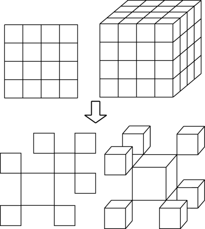
Figure 1: Husimi lattice (HL) and the cubic recursive lattice (CRL) constructed from the basic units of regular lattices.

II.2 Multi-branched Recursive Lattice

As mentioned above, the HL with $q=4$ is formed by connecting two square units of the regular square lattice of the same $q$, and it is the same for the CRL of $q=6$ to describe the regular cubic lattice. This may cause a misunderstanding that the recursive lattice of a given coordination number $q$ can only be constructed from the single unit of a regular lattice with that particular $q$, which is not true. It should be recognized that the coordination number alone does not determine the structure of basic unit. For example, we can modify the original HL by joining three square units at one vertex, as shown in Fig. 2, to result in $q=6$. This is made possible by the independence of units in recursive lattice. In this case, we may ask the following questions: Is this modified HL, with three branches joint on one vertex, also capable to approximate a 3-D regular lattice like the CRL based on the same $q$? If yes, what advantages or disadvantages does it hold, compared to the CRL? These questions will be investigated in this work.

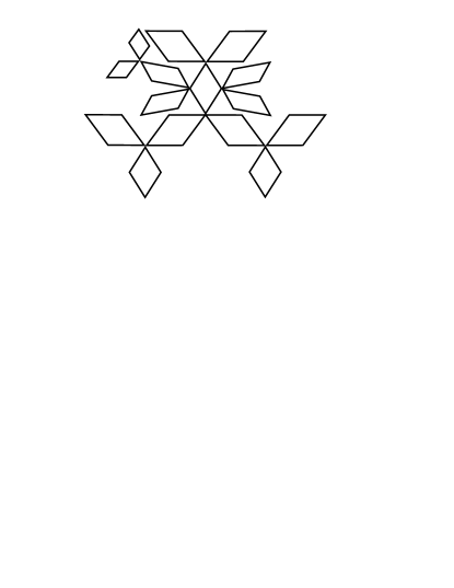
Figure 2: A 3-branched Husimi lattice with $q=6$. Note that all the units are square and equal in size, however they cannot be drawn in that way on page.

III Antiferromagnetic Ising Model

An Ising spin $S$ has two possible values, which usually are assigned as $+1$ (up or $+$) and $-1$ (down or $-$) Ising ; Onsager ; Wu , and they can represent a particle and the void in a monatomic system, or particle A and B in an alloy. The Ising model with the nearest-neighbor interactions between neighboring spins $S_{i}$ and $S_{j}$ and in the presence of an external magnetic field $H$ has the energy given by

$$E=-J{\sum_{<i,j>}}S_{i}S_{j}-H{\sum}S_{i},$$

where $<i,j>$ is the nearest-neighbor pairs of lattice sites $i$ and $j$, and $S_{i}=\pm 1$ is the spin on the site $i$. The value of $J$ can be setup to be either positive or negative. For the $J>0$ case, the spins in the same state (the parallel arrangement) will have the lowest energy at absolute zero, so that the model has a ferromagnetic ordering. Vice versa, the anti-parallel arrangement at absolute zero is favored by the antiferromagnetic interaction $J<0$.

We will take the antiferromagnetic interaction in this paper for two reasons: (1) The ferromagnetic case prefers only one spin state aggregated together at the near-zero temperature, which implies a total phase separation of two particles A and B in the alloy case, or a compressible pure system ruling out all the voids. On the other hand, the antiferromagnetic case provide a uniform state at low temperature, which is facilitated for us to investigate the equilibrium thermodynamics; (2) While the ferromagnetic case has only one solution, the antiferromagnetic interaction can provide two solutions representing the stable and metastable states, which is necessary to study the supercooled liquid and glass transition. The details of this so-called “solutions” will be discussed later.

The standard Ising model only includes the interaction between the nearest neighbor spins. Nevertheless, it is not realistic that particles farther away than the nearest distance do not interact with each other in real systems. For a better approximation of a real system, more interaction energy terms such as the interactions between second neighbor sites, interaction between three and four spins are also considered in our model.

IV Model, Fix-point solutions and Thermodynamics

The calculation of HL and CRL are similar in principle. As a basic unit cell at a higher level shares a single site connecting it to the lower level, this site in each unit plays a role different from the other sites. We will call this the base site and the corresponding spin at that site will be generically denoted by $S^{\text{b}}$. In particular, we can define the energy $e_{\alpha}$ associated with a cell $\alpha$ by paying special attention to this site in such a way that the sum over all cells will give the energy $E$ of the model over the entire recursive lattice. Here we will take the multi-branched HL for example to demonstrate the calculation method, and briefly give the generalized formula for CRL, for which the details of calculations were described in our previous works, e. g. the Ref. PDG4 . We will, however, present all relevant details here.

IV.1 Spins Conformation

We first consider a HL made up by squares as the unit cells. The four spins in such a square with its base site at the $m$-th level are shown in Fig. 3a, with $S_{m}$ as the base site. The peak site is at level $m+2$ and the remaining intermediate sites are at level $m+1$. The spins at the intermediate sites are denoted by $S_{m+1}$ and $S_{m+1}^{\prime}$, respectively. The energetic of the model is defined by considering these squares. We now introduce following quantities for a square cell:

$$A_{\text{mag}} =S_{m+1}+S_{m+1}^{\prime}+S_{m+2};$$

$$A_{\text{nb}} =S_{m}S_{m+1}+S_{m}S_{m+1}^{\prime}+S_{m+1}S_{m+2}+S_{m+1}^{\prime}S_{m+2};$$

$$A_{\text{sd}} =S_{m}S_{m+2}+S_{m+1}S_{m+1}^{\prime};$$

$$A_{\text{tri}} =S_{m}S_{m+1}S_{m+1}^{\prime}+S_{m}S_{m+1}^{\prime}S_{m+2}+S_{m}S_{m+1}S_{m+2}+S_{m+1}S_{m+1}^{\prime}S_{m+2};$$

$$A_{\text{qua}} =S_{m}S_{m+1}S_{m+1}^{\prime}S_{m+2}.$$

Note that the base site is not included in the magnetic term $A_{\text{mag}}$; instead we only count the contributions from the sites of the unit cell above the site $S_{m}$. The missing contribution from this site will be accounted in the next unit on lower level, when we construct the recursion relations below.

Let $\gamma$ denote a particular spin state in the cell. The energy of the Ising model in the cell for a particular cell state $\gamma$ is:

$$e(\gamma)=-JA_{\text{nb}}(\gamma)-J_{P}A_{\text{sd}}(\gamma)-J^{\prime}A_{\text{tri}}(\gamma)-J^{\prime\prime}A_{\text{qua}}(\gamma)-HA_{\text{mag}}(\gamma),$$ (1)

where $J_{P}$ is the interaction energy between the second nearest sites, $J^{\prime}$ is the interaction energy of three sites (triplet), and $J^{\prime\prime}$ is the interaction energy of the four sites (quadruplet).

The total energy of the Ising model mentioned above is the sum of the energy of all cells $\alpha$ on our recursive lattice:

$$E(\Gamma)={\textstyle\sum_{\alpha}}e(\gamma_{\alpha})-HS_{0},$$ (2)

where $\Gamma={\textstyle\bigotimes\nolimits_{\alpha}}\gamma_{\alpha}$ denotes the spin state of the lattice, and $S_{0}$ now represents the spin at the origin of the recursive lattice. It should be addressed here that, since our lattices are homogeneous and infinitely large, any site on the lattice can be artificially selected to be the origin site. There are four sites in a square cell; hence, the number of possible states of a cell is $2^{4}=16$. The 1st to the 8th states correspond to the base spin $S_{m}=+1$, and the 9th to the 16th states to $S_{m}=-1$ on the base site. The number of lattice conformations $\Gamma$ for a lattice with $N_{\text{C}}$ cells is $16^{N_{\text{C}}/r}$, where the coefficient $r$ is the number of branches joined at one site for a multi-branched lattice.

Note that in this paper the temperature $T$ and $\beta=1/T$ are normalized with Boltzmann constant $k_{B}=1$. The Boltzmann weights are given by

$$w(\gamma)=exp(-\beta e(\gamma)),\ w(\Gamma)=\exp(\beta HS_{0}){\textstyle\prod\nolimits_{\alpha}}w(\gamma_{\alpha}).$$ (3)

Then the partition function (PF) is a sum over lattice configurations:

$$Z(T)=\underset{\Gamma}{\sum}w(\Gamma).$$ (4)

By choosing proper values of the interaction energies, we can simulate various systems to study their thermodynamics and phase transitions under different conditions. As a convention, we take $J=-1$ to set the temperature scale for our model.

IV.2 Fix-point solution

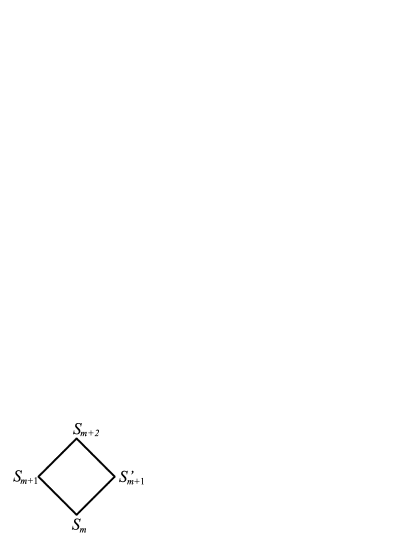
(a)

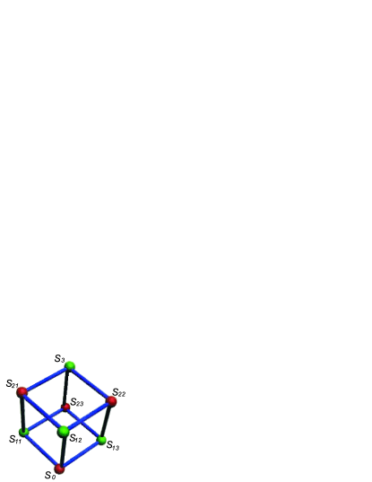
(b)

Figure 3: Level index and sites labeling in the (a) square and (b) cubic unit.

Since the units are connected together only at a site, the units on higher levels from some site may be treated as a branch linked to a particular site. The branch $\mathcal{T}_{m}$ is obtained by cutting the lattice at the $m$-th site; see in Fig. 4. This branch is said to have its base site at the $m$-th level. A partial partition function (PPF) $Z_{m+1}(S_{m+1})$ for the branch $\mathcal{T}_{m+1}$ with its base at the level $m+1$ can be introduced to represent the contribution of the branch with spin $S_{m+1}$ fixed as its base site. Then the PPF $Z_{m}(S_{m})$ at the lower level $m$ can be expressed in terms of PPF’s $Z_{m+1}(S_{m+1})$, $Z_{m+1}(S_{m+1}^{\prime})$, and $Z_{m+2}(S_{m+2})$ at higher levels. Thus, recursively we can start from an initial site to calculate the contribution of the entire lattice towards the origin. In this way, we can obtain the thermodynamics of the entire system.

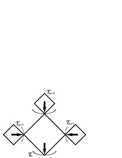
Figure 4: Contributions of sub-branches in the HL.

The partition function $Z_{0}$ of the lattice can be represented by the contributions to the origin site from the $r$ branches $T_{0}$ meeting at the origin with either $S_{0}$:

$$Z_{0}=Z_{0}^{r}(+)e^{\beta H}+Z_{0}^{r}(-)e^{-\beta H}$$ (5)

The weights of the magnetic field above is due to the contribution from the base site, which is not included in $A_{\text{mag}}$.

We now turn to the PPF’s. As each PPF at a base site in the square is a sum of the $8$ configurations of the remaining three sites in the square, with $r^{\prime}\equiv r-1$ we have

$$Z_{m}(+) =\underset{\gamma=1}{\overset{8}{\sum}}Z_{m+1}^{r^{\prime}}(S_{m+1})Z_{m+1}^{r^{\prime}}(S_{m+1}^{\prime})Z_{m+2}^{r^{\prime}}(S_{m+2})w(\gamma),$$ (6)

$$Z_{m}(-) =\underset{\gamma=9}{\overset{16}{\sum}}Z_{m+1}^{r^{\prime}}(S_{m+1})Z_{m+1}^{r^{\prime}}(S_{m+1}^{\prime})Z_{m+2}^{r^{\prime}}(S_{m+2})w(\gamma),$$ (7)

with a product from the $r^{\prime}$ branches at the two sites on level $m+1$ and the $r^{\prime}$ branches at the peak site at $m+2$.

We now introduce the ratios

$$x_{m}=\frac{Z_{m}(+)}{Z_{m}(+)+Z_{m}(-)},\ y_{m}=\frac{Z_{m}(-)}{Z_{m}(+)+Z_{m}(-)}.$$ (8)

and

$$z_{m}(S_{m})=\left\{\begin{array}[c]{c}x_{m}\text{ if }S_{m}=+1\\ y_{m}\text{ if }S_{m}=-1\end{array}\right.$$ (9)

In terms of

$$B_{m}^{r\prime}=Z_{m}(+)+Z_{m}(-),$$

we have $Z_{m}(+)=B_{m}^{r\prime}x_{m}$ and $Z_{m}(-)=B_{m}^{r\prime}y_{m}$. By use of (9), we obtain

$$B_{m}^{r\prime}z_{m}(\pm) =\sum B_{m+1}^{r\prime}z_{m+1}^{r^{\prime}}(S_{m+1})B_{m+1}^{r\prime}z_{m+1}^{r^{\prime}}(S_{m+1}^{\prime})B_{m+2}^{r\prime}z_{m+2}^{r^{\prime}}(S_{m+2})w(\gamma),$$

$$z_{m}(\pm) =\sum z_{m+1}^{r^{\prime}}(S_{m+1})z_{m+1}^{r^{\prime}}(S_{m+1}^{\prime})z_{m+2}^{r^{\prime}}(S_{m+2})w(\gamma)/Q(x_{m+1},x_{m+2}),$$

where the sum is over $\gamma=1$, $2$, $3$, …, $8$ for $S_{m}=+1$, and over $\gamma=9$, $10$, $11$, …, $16$ for $S_{m}=-1$, and where

$$Q(x_{m+1},x_{m+2})\equiv\left[B_{m}/B_{m+1}^{2}B_{m+2}\right]^{r^{\prime}};$$

it is related to the polynomials

$$Q_{+}(x_{m+1},x_{m+2}) =\underset{\gamma=1}{\overset{8}{\sum}}z_{m+1}^{r^{\prime}}(S_{m+1})z_{m+1}^{r^{\prime}}(S_{m+1}^{\prime})z_{m+2}^{r^{\prime}}(S_{m+2})w(\gamma),$$

$$Q_{-}(x_{m+1},x_{m+2}) =\underset{\gamma=9}{\overset{16}{\sum}}z_{m+1}^{r^{\prime}}(S_{m+1})z_{m+1}^{r^{\prime}}(S_{m+1}^{\prime})z_{m+2}^{r^{\prime}}(S_{m+2})w(\gamma),$$

according to

$$Q(x_{m+1},x_{m+2})=Q_{+}(x_{m+1},x_{m+2})+Q_{-}(y_{m+1},y_{m+2}).$$

In terms of the above polynomials, we can express the recursive relation for the ratio $x_{m}$ in terms of $x_{m+1}$ and $x_{m+2}$:

$$x_{m}=\frac{Q_{+}(x_{m+1},x_{m+2})}{Q(x_{m+1},x_{m+2})}.$$ (10)

A similar relation holds for $y_{m}\equiv 1-x_{m}$:

$$y_{m}=\frac{Q_{-}(y_{m+1},y_{m+2})}{Q(y_{m+1},y_{m+2})}.$$ (11)

Clearly from the definition of $x$, the physical meaning of the solution is the ratio of sub-trees’ thermodynamic contributions to a particular site (excluded), i.e. the cavity magnetization cavity , therefore it determines the probability that a site is occupied by the spin $S=+1$, and we can subsequently take it to be the solution of the entire lattice. Because of the recursive property of these equations, we would expect the cycle-form solutions, which is called the fix-point (FP) solution. Then the bulk thermodynamic calculation just focuses on solving the Eqs. (10, 11) and determine the FP solution. In this work, our calculation provides two types of solutions for each model, the alternating state solution (2-cycle) and the uniform solution (1-cycle). At high temperatures, we find a uniform FP solution $x$ on all the sites, which we call the 1-cycle solution:

$$x=\frac{Q_{+}(x,x)}{Q(x,x)}.$$

At low temperatures, we find alternating solutions $x_{1}$ and $x_{2}$ on the two successive levels, which we call a 2-cycle solution:

$$x_{1}=\frac{Q_{+}(x_{2},x_{1})}{Q(x_{2},x_{1})},\ x_{2}=\frac{Q_{+}(x_{1},x_{2})}{Q(x_{1},x_{2})}.$$

This describes the antiferromagnetic ordering, i.e. two neighboring spins prefer to be in different states at low temperature. In contrast, the 1-cycle solution represents the less-ordered state, in which all the spins have the same probability to be in either states. Based on the nature of antiferromagnetic Ising model, a three or higher cycle solutions is hard to imagine. And although we cannot prove that there is no solution other than the 1- and 2-cycle form, we have not found any. The details of solutions will be discussed in the later section.

IV.3 Calculation of thermodynamics

IV.3.1 Free Energy

It is clear that the 1-cycle solution is a special case of the 2-cycle solution with $x_{1}=x_{2}$. Therefore, we will assume a 2-cycle solution and determine its thermodynamics in this section. If it happens that $x_{1}=x_{2}$, we obtain the 1-cycle thermals. The solution with a higher free energy will then describe a metastable state, which will be useful to identify the supercooled liquid and the glass transition.

The Helmholtz free energy is given by

$$F=-T\log Z$$

and requires obtaining the partition function $Z$, which is given by Eq. (5). As the lattice is infinitely large, there is no sense in calculating $Z$ or $F$, each of which will also be infinite. At the FP solution, we can use its homogeneity over two levels to obtain the free energy per site by following the Gujrati trick [11], which we briefly describe below. We consider the HL made up by connecting $r$ squares at each site. The partition function of the whole system is given by considering the $r$ branches $\mathcal{T}_{0}$ meeting at the origin as shown in Fig. 5.

Imagine that we cut off the $rr^{\prime}$ branches $\mathcal{T}_{2}$ on level 2 and hook up them together to form $r^{\prime}$ smaller lattices. The partition function of each of these smaller lattices is:

$$Z_{2}=Z_{2}^{r}(+)e^{\beta H}+Z_{2}^{r}(-)e^{-\beta H}.$$

Similarly we can imagine to cut off the $2rr^{\prime}$ branches $\mathcal{T}_{1}$ and hook them up to form $2r^{\prime}$ smaller lattices. The partition function of each smaller lattice is

$$Z_{1}=Z_{1}^{r}(+)e^{\beta H}+Z_{1}^{r}(-)e^{-\beta H}.$$

Since free energy is an extensive quantity, the free energy of the whole system is the sum of the free energies of the smaller lattices and the $r$ local squares that are left out after dissecting the original lattice. The free energy of the left out squares is

$$F_{local}=-T\log\left[\frac{Z_{0}}{(Z_{1}^{2}Z_{2})^{r^{\prime}}}\right].$$

There are $4/r$ cites per square and $r$ squares in the local region. Thus, the free energy per site is:

$$F=-\frac{F_{local}}{4}.$$ (12)

By substituting $Z_{m}(+)=B_{m}x_{m}$ and $Z_{m}(-)=B_{m}y_{m},$ we finally obtain

$$F=-\frac{1}{4}T\log(Q^{2r^{\prime}}\frac{1}{\{[x_{1}^{r}e^{\beta H}+(1-x_{1})^{r}e^{-\beta H}]^{2}[x_{2}^{r}e^{\beta H}+(1-x_{2})^{r}e^{-\beta H}]\}^{r^{\prime}}})$$ (13)

Using the FP solution $x_{1}$ and $x_{2}$ from the FP calculation, the numerical value of free energy can be easily achieved.

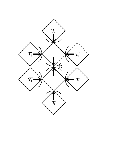
Figure 5: Two squares meeting at the origin of the lattice. In general, there are $r$ units meeting at the origin.

IV.3.2 Conformation Probability

A square unit with 4 spins on each site has sixteen possible conformations $\gamma$. The probability of a given conformation $\gamma$ is

$$P(\gamma)=\frac{\left[Z_{0}(S_{0})Z_{1}(S_{1})Z_{1}(S_{1}^{\prime})Z_{2}(S_{2})\right]^{r^{\prime}}\exp(\beta HS_{0})w(\gamma)}{Z_{0}},$$

which satisfies the sum rule

$$\overset{16}{\underset{\Gamma}{\sum}}P(\gamma)=1.$$

It is easy to obtain that

$$P(\gamma)=\frac{\left[z_{0}(S_{0})z_{1}(S_{1})z_{1}(S_{1})z_{2}(S_{2})\right]^{r^{\prime}}\exp(\beta HS_{0})w(\gamma)}{Q_{{}_{+}}x_{0}^{r}e^{\beta H}+Q_{{}_{-}}(1-x_{0})^{r}e^{-\beta H}}$$

IV.3.3 Energy Density

The energy density is defined as the summation over the product of the energy and the probability of a conformation state. Once we have the conformation probabilities $P(\gamma)$, energy density (per site) can be simply calculated by evaluating the sum of the product of energy of each conformation and the $P(\gamma)$:

$$E=\frac{r}{4}{\textstyle\sum}e(\gamma)P(\gamma)$$

where

$$e_{\alpha}=-JA_{nb}-J_{P}A_{\text{sd}}-J^{\prime}A_{\text{tri}}-J^{\prime\prime}A_{\text{qua}}-H(S_{\alpha}^{\text{b}}+A_{\text{mag}})/r$$

is the energy of a unit cell $\alpha$ in a configuration $\gamma$ as mentioned before. The base site $S_{\alpha}^{\text{b}}$ is included in the magnetic term as it contributes to the energy of each cell.

IV.3.4 Entropy

With the free energy and energy density, by definition we simply have the entropy as

$$S=\beta(E-F),$$

or from the first derivative of the free energy with respect to the temperature:

$$S=-\partial F/\partial T.$$

Depends on the setup of energy parameters, the entropy obtained from 1-cycle solution is possible to be zero at some temperature $T_{\text{K}}$ below the melting transition temperature $T_{\text{M}}$, since it represents the metastable supercooled liquid. The entropy will become negative below $T_{\text{K}}$ with continuous cooling. However negative entropy is known as unphysical in nature, thus the metastable state must undergo a transition and change to the glass state before $T_{\text{K}}$, which in this way is defined as the ideal glass transition temperature.

IV.4 The CRL calculation

The CRL calculation is similar to the method introduced in the previous section and can be found in Ref. Ran1 . Here we briefly give the scheme of the CRL calculation. In a CRL the sites on a cube unit are divided into four layers and labeled as follows: $S_{m}$, $(S_{m+1,1}$, $S_{m+1,2}$ , $S_{m+1,3})$, $(S_{m+2,1}$, $S_{m+2,2}$, $S_{m+2,3})$, and $S_{m+3}$; see Fig. 3b where we take $m=0$. The sub-tree contributions in the CRL are demonstrated in Fig. 6.

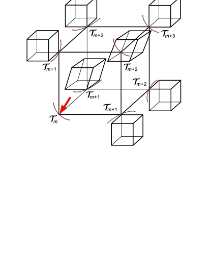
Figure 6: The sub-tree contributions in the CRL.

Taking their contributions at each site easily gives the recursion relations for the PPFs:

$$Z_{m}(+) =\underset{\gamma=1}{\overset{128}{\sum}}[\overset{3}{\underset{\{m+1\}}{\prod}}Z_{m+1}(S_{m+1})][\overset{3}{\underset{\{m+2\}}{\prod}}Z_{m+2}(S_{m+2})]Z_{m+3}(S_{m+3})w(\gamma),$$

$$Z_{m}(-) =\underset{\gamma=129}{\overset{256}{\sum}}[\overset{3}{\underset{\{m+1\}}{\prod}}Z_{m+1}(S_{m+1})][\overset{3}{\underset{\{m+2\}}{\prod}}Z_{m+2}(S_{m+2})]Z_{m+3}(S_{m+3})w(\gamma),$$

By introducing $B_{m}$ and the ratios $x_{m}$, $y_{m}$, and $z_{m}(S_{m})$ (Eq. 9) as before, we have

$$Q_{+}(x_{m+1},x_{m+2},x_{m+3}) =\underset{\gamma=1}{\overset{128}{\sum}}[\overset{3}{\underset{\{m+1\}}{\prod}}z_{m+1}(S_{m+1})][\overset{3}{\underset{\{m+2\}}{\prod}}z_{m+2}(S_{m+2})]z_{m+3}(S_{m+3})w(\gamma),$$

$$Q_{-}(x_{m+1},x_{m+2},x_{m+3}) =\underset{\gamma=129}{\overset{256}{\sum}}[\overset{3}{\underset{\{m+1\}}{\prod}}z_{m+1}(S_{m+1})][\overset{3}{\underset{\{m+2\}}{\prod}}z_{m+2}(S_{m+2})]z_{m+3}(S_{m+3})w(\gamma),$$

and

$$Q(x_{m+1},x_{m+2},x_{m+3})=Q_{+}(x_{m+1},x_{m+2},x_{m+3})+Q_{-}(y_{m+1},y_{m+2},y_{m+3})=\frac{B_{m}}{B_{m+1}^{3}B_{m+2}^{3}B_{m+3}}.$$

We can now obtain the recursive relation for the ratio $x_{m}$ in terms of $x_{m+1}$, $x_{m+2}$ and $x_{m+3}$:

$$x_{m}=\frac{Q_{+}(x_{m+1},x_{m+2},x_{m+3})}{Q(x_{m+1},x_{m+2},x_{m+3})}.$$

A similar relation holds for $y_{m}\equiv 1-x_{m}$:

$$y_{m}=\frac{Q_{-}(y_{m+1},y_{m+2},y_{m+3})}{Q(y_{m+1},y_{m+2},y_{m+3})}.$$

For the CRL case, we also have the 1-cycle solution, $x_{m}=x_{m+1}=x_{m+2}=x_{m+3}$, which represents the disordered state, and the 2-cycle solution, $x_{m}=x_{m+2}$ and $x_{m+1}=x_{m+3}$, which represents the ordered stable state. Thermodynamic properties such as free energy and entropy can be calculated from the solutions using similar techniques as before. The local area around the origin is chosen to be the two cubes joint on the origin site, and it has eight sites. The final expression of the free energy per site is:

$$F=\frac{1}{8}F_{local}=-\frac{1}{8}T\log(Q^{2}\frac{1}{[x_{1}^{2}e^{\beta H}+(1-x_{1})^{2}e^{-\beta H}]^{4}[x_{2}^{2}e^{\beta H}+(1-x_{2})^{2}e^{-\beta H}]^{2}})$$ (14)

V Results and Discussion

The thermodynamic calculations have been done on 3-branched HL ($r=3$) and CRL. Since both models are to approximate the 3-D regular lattice, the results will be compared in this section. The role of energy parameters will be studied in both cases. In the following discussion, we will call the parameters setup of $J=-1$ and all other parameter to be zero as the reference case.

V.1 General solutions with $J=-1$ and all other parameter are zero

The reference 1- and 2-cycle solutions of the original HL, HL of $r=3$, and CRL are shown in Fig. 7. We can see that the 1-cycle solutions of all the models are $x=0.5$ everywhere, which implies that the probability of a site occupied by $S=+1$ is simply fifty percent with the absence of magnetic field $H$ in the Hamiltonian. This situation corresponds to a disordered phase and represents a high free energy state at low temperature (the supercooled liquid) 23 . For the 2-cycle solutions, one branch approaches to $1$ and the other approaches to $0$ as $T\rightarrow 0$, thus we have $S=+1$ and $S=-1$ alternatively occupying the two neighboring sites at low $T$. This structure represents the ordered states (crystal) and is characterized by the complete antiferromagnetic order in the Ising model.

To clarify more about the physical meaning the solutions in our model: The 2-cycle solution is the most ordered state at a particular temperature, subsequently it is the crystal; Meanwhile, the 1-cycle is the “most disordered state”, i.e. an antiferromagnetic Ising model cannot be more disordered with fifty percent probability of spins states everywhere. However, since it is still an achievable solution, it should be taken as the upper limit of the amorphous states, i.e. the most unstable state out of all the possible states. In this way, any artificial values between 0 and 1 of solutions $x_{1}$ and $x_{2}$ with summation of 1 correspond to a possible state of the system. In the next section, the thermodynamics of 1-cycle solution will be discussed and it behaves exactly as the supercooled liquid and exhibits the Kauzmann paradox, which agrees with our expectation that this less stable solution is the metastable one.

At a critical temperature $T=2.75$, the 2-cycle solution turns to be 1-cycle and there occurs a transition for the original HL, where the crystal state turns into the disordered state. This represents the melting transition $T_{\text{M}}$ 24 ; 25 from crystal to liquid. For the HL of $r=3$, the melting temperature increases significantly and becomes very close to the one in CRL. The $T_{\text{M}}$ is found to be 4.84 in CRL and 4.89 in the 3-branched HL. These values are comparable to the results obtained by other methods on the Ising antiferromagnetic model on a simple cubic lattice: 4.51 by Monte Carlo 26 , 4.93 by mean field renormalization group 27 and 4.52 by series expansion 28 . This adds faith that our model is not far from a realistic model. We can observe that the singular temperature moves towards the ”correct” temperature 4.51 or 4.52 obtained by simulation or series analysis as we increase the coordination number in the case of the two HLs, or use a more realistic unit cell (the cube). Meanwhile, they drift away from the mean field renormalization group result.

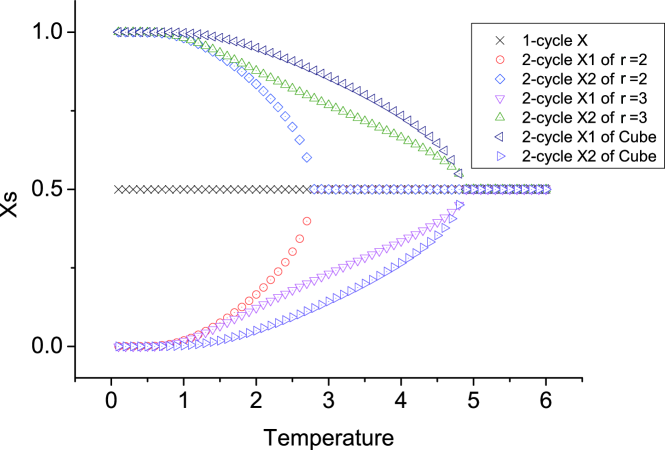
Figure 7: The reference 2-cycle and the 1-cycle solutions of original HL, HL of $r=3$, and CRL ($J=-1$ and other parameters are zero).

The difference between the 2-cycle solutions in both lattices is also remarkable. It is as expected that HL of $r=3$ is better to describe the 3-D case than the HL of $r=2$. However, in Fig. 7, the curves of $x$s of the $r=3$ HL are more like the stretched curves of the original HL solutions, while the $x$s of CRL are more rounded curves. The difference between $x_{0}$ and $x_{1}$ is larger in CRL. Since the 1 and 0 cyclic solution at the zero temperature corresponds to the ideal crystal stable state, a 2-cycle can be identified to be more stable if its two branches are closer to 1 and 0 respectively, by this meaning the 2-cycle solution in CRL is more stable below $T_{\text{M}}$ than in the 3-branched HL. This difference can also be observed in the thermal properties discussed below.

V.2 Thermodynamics of $r=3$ HL and CRL with reference case

Figure 8 and 9 show the thermodynamics of $r=3$ HL and CRL with reference case. Basically, like the behaviors of solutions, the two models exhibit similar thermal behaviors with slight difference. Herein, we will discuss the general transitions occurring on each type of solution, and re-examine the properties of models those have been concluded from the solutions.

For the 2-cycle solutions, there is merely the melting process that can be observed. At the melting transition, the entropy of 2-cycle solution falls dramatically due to the crystallization, The rapid drop in the entropy of the 2-cycle reflects that the simple Ising model, which we will call the reference model in this work, is not realistic enough to give a discontinuous melting. Although a continuous transition seems contradicting to the general idea of “melting process”as a first-order transition, the phenomenon of transition from the ordered to the disordered state should still be treated as the melting process. Further studies also confirm that particular parameters setup can produce a discontinuous transition for the 2-cycle case, this part will not be detailed in this paper.

On the other hand, following the behavior of the supercooled liquid, with the cooling process the entropy of 1-cycle solution continues to decrease gradually at and below $T_{\text{M}}$, and there occurs no transition. At some point, the entropy of the supercooled liquid decreases faster than the crystal, and rapidly goes below the crystal entropy then to negative values, which demonstrates the Kauzmann paradox Kauzmann ; Debenedetti , i.e. the ideal glass transition.

The Kauzmann paradox was originally referred to where the entropy of supercooled liquid becomes lower than the crystal entropy. This is because that, at the same temperature the kinetic (vibration) entropy of crystal and supercooled liquid are the same, and the entropy of crystal was approximated to be the kinetic entropy, then the difference between the entropy of crystal and supercooled liquid, i.e. the excess entropy, equals to the configurational entropy, which cannot be negative. However, the entropy of crystal at non-zero temperature is not only contributed by the kinetic entropy, it also has entropy from defects. In this way it is possible to have a supercooled liquid state with less defects and lower entropy than the crystal state at the same temperature. Therefore, we will simply take the negative entropy of the supercooled liquid as the paradox, and the temperature where negative $S$ occurs is defined as the Kauzmann temperature $T_{\text{K}}$. This clarification is important, since in later section we will show a special case, in which we still have negative excess entropy but the negative entropy itself vanishes.

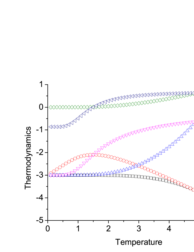
Figure 8: The reference thermal properties of the 2-cycle and 1-cycle case for $r=3$ HL ($J=-1$ and other parameters are zero).

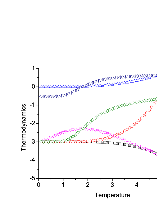
Figure 9: The reference thermal properties of the 2-cycle and 1-cycle case for CRL ($J=-1$ and other parameters are zero).

V.3 The effect of $J_{p}$

Beside the interaction $J$ between the nearest spins, the interactions between spins farther apart also play important roles in our lattice model. With the set of various values of these parameters, the model is capable to simulate many different cases, i.e. to manipulate the transition temperatures. As we modify the interaction along the surface diagonal $J_{P}$, it significantly changes the transition temperatures as shown in Figs. 10.

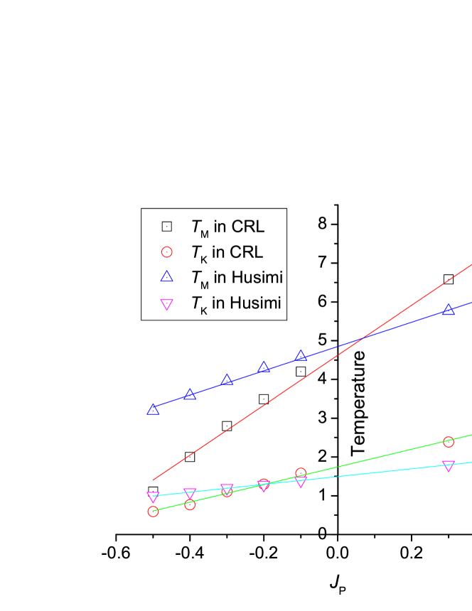
Figure 10: The transition temperature variation with different $J_{P}$ in CRL and the HL of $r=3$.

In both lattices, the increment of $J_{P}$ enhances the transition $T$ in a linear relationship. From Eq. 1 it is easy to understand that the negative value of $J_{P}$ competes with negative $J$. The negative $J$ prefers different states of the nearest spins and consequently the same states of the spins on the surface diagonal, while negative $J_{P}$ forces the diagonal spins to be in different states. Thus, in both the CRL and HL the decrease of $J_{P}$ lowers the transition temperature, that is, makes the system unstable and easier to undergo a transition. On the other hand, positive $J_{P}$ favors antiferromagnetic spin configuration and increases the transition temperature for the same reason. In CRL, the role of $J_{P}$ is more significant than it is in the HL, because a cubic unit has 12 surface diagonal interactions and 12 nearest neighbor interactions, while a square unit has 4 $J$’s and 2 $J_{P}$’s therefore the diagonal interactions have less weight.

V.4 The effect of $J^{\prime}$

An important feature of $J^{\prime}$ is that its sign (positive or negative) does not affect the solutions. With the increase of $J^{\prime}$, the transition temperatures decrease by a small slope in the CRL, and even smaller in the HL. That is because the three-spins interactions would disturb the ordered state formation; nevertheless its contribution is very small in the total energy in either cases (Fig. 11).

Another interesting effect of $J^{\prime}$ is that, although the transition temperature changes weakly with $J^{\prime}$, it changes the thermodynamic curves dramatically, and with $J^{\prime}=1$ it could even destroy the ideal glass transition by having the supercooled liquid entropy positive till zero temperature, as shown in Fig. 12. In this situation, we still have the original Kauzmann paradox without permitting the lower entropy of supercooled liquid than the crystal, nevertheless by our definition the negative entropy vanishes and the paradox does not hold anymore.

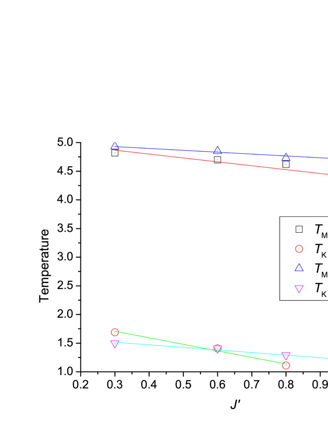
Figure 11: The transition temperature variation with different $J^{\prime}$ in CRL and the HL of $r=3$.

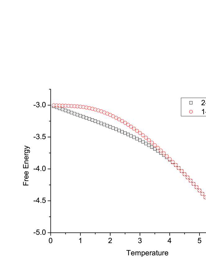
(a)

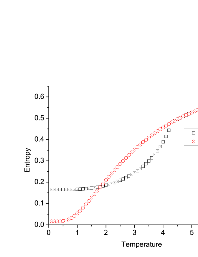
(b)

Figure 12: The (a) free energy and (b) entropy of the extraordinary case of CRL model with $J^{\prime}=1$. The Kauzmann paradox vanishes for the 1-cycle solution.

V.5 The effect of $J^{\prime\prime}$

The roles of four-spins interaction $J^{\prime\prime}$ in CRL and HL are very different. There are six squares in one cubic unit in the CRL. The value of $J^{\prime\prime}$ affects the spins states in the same way as $J_{P}$, i.e. it increases the transition temperature. However it does not change $T_{\text{M}}$ and $T_{\text{K}}$ in the HL because the 4-spins interaction is mainly the interaction of the whole unit, thus its effect is like a magnetic field $H$ for each single spin (Fig. 13).

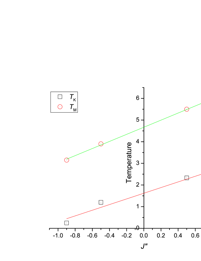
Figure 13: The transition temperature variation with different $J^{\prime\prime}$ in CRL.

VI Conclusion

The Ising model on a recursive lattice enables us to do exact calculations without approximation to study the supercooled liquid, the crystal formation and phase transitions. We have constructed and compared a multi-branched 2-D HL and a cubic recursive lattice of the same coordination number $q$. The branch number is set to be 3 in the multi-branched 2-D HL to make $q$ to be 6. Because of the identical $q$, both lattice are designed to approximate the regular 3-D lattice. We applied the antiferromagnetic Ising model on the two lattices, in which the alternative spin arrangement represents the ordered phase (crystal state), while the homogeneous spins arrangement represents the metastable state, i.e. the liquid and the supercooled liquid states.

A set of solutions relating to the probability that one site being occupied by a particular spin state can be exactly calculated on the lattice from the ratio of partial partition functions. Two types of solutions, representing the ordered and disordered states respectively, give the thermodynamics of crystal and metastable states. The behavior of the free energy and the entropy of two states allows us to locate the melting transition at $T_{\text{M}}$ and the Kauzmann temperature $T_{\text{K}}$. The $T_{\text{M}}$ is determined by the differing of two states with temperature decreasing (cooling process), above $T_{\text{M}}$ the two solutions have the same disordered behavior as liquid. When the system goes below $T_{\text{M}}$, an ordered state (from 2-cycle solution) appears with lower free energy and entropy, while the disordered solution (1-cycle) still exists and the system is possible to continue in supercooled state without phase transition. The entropy of this disordered state gradually decreases to zero and then becomes negative at a non-zero temperature, which is determined to be the ideal glass transition temperature, or Kauzmann temperature $T_{\text{K}}$.

The transition temperatures determined on both lattices are very close to each other, and fairly agree with the results from other methods such as MC simulation and series analysis. The results confirm our expectation that: (1) The CRL is a good approximation of regular 3-D cubic lattice; (2) With the same coordination number the multi-branched 2-D HL is also capable to describe systems in higher dimension. It is also concluded that the 3-branched Husimi lattice provides a less versatile and accurate method compared to the CRL. For example, the CRL provides a transition temperature closer to that obtained by series analysis than the one obtained by the HL. However, the multi-branched HL calculation is simpler and less time-consuming, which still holds merits in applications.

In addition to the nearest neighbor interactions, the effects of second nearest interaction, triplet and quadruplet interaction are also studied in this work. All their effects are similar for the two lattices except $J^{\prime\prime}$. This enables us to obtain expected transition temperature or thermodynamic behaviors by adjusting the interaction parameters for an extensive use of our models.

References

- (1) W. Kauzmann, Chemical Reviews 43, 2 (1948).
- (2) The Class Transition and the Nature of the Glassy State, edited by M. Goldstein and R. Simha, Ann. N. Y. Acad. Sci. 279 (1976).
- (3) W. Gotze, Liquids, Freezing and the Glass Transition, edited by J. P. Haasma, D. Levesque, and J. Zinn-Justin, North-Holland, Amsterdam (1991).
- (4) P. G. Debenedetti, Metastable Liquids: Concepts and Principles, Princeton University Press, Princeton, New Jersey (1996).
- (5) M. Mézard and G. Parisi, J. Phys.: Condense. Matter. 12 6655 (2000).
- (6) P. G. Debenedetti and F. H. Stillinger, Nature 410, 259 (2001).
- (7) H. A. Bethe, Proc. Roy. Soc. London Ser A 150, 552 (1935).
- (8) K. Husimi, J. Chem. Phys. 18, 682 (1950).
- (9) P. D. Gujrati, Phys. Rev. Lett. 74, 809 (1995).
- (10) J. Ryu and P. D. Gujrati, J. Chem. Phys. 107, 1259 (1997).
- (11) P. D. Gujrati, J. Chem. Phys. 108, 5089 (1998).
- (12) F. Semerianov and P. D. Gujrati, Phys. Rev. E 72, 011102 (2005).
- (13) R. J. Baxter, Exactly Solved Models in Statistical Mechanics, Academic Press, London (1982) 1st ed., p. 47.
- (14) A. J. Banchio and P. Serra, Phys. Rev. E 51, 2213 (1995).
- (15) R. A. Zara and M. Pretti, J. Chem. Phys. 127, 184902 (2007).
- (16) J. A. Verges and F. Yndurain, J. Phys. F: Met. Phys. 8, 873 (1978).
- (17) W. Geertsma and J. Dijkstra, J. Phys. C: Solid State Phys. 18, 5987 (1985).
- (18) J. F. Stilck and M. J. de Oliveira, Phys. Rev. A 42, 5955 (1990).
- (19) R. Huang and C. Chen, Commun. Theor. Phys. 62, 749 (2014).
- (20) E. Ising, Z. Phys. 31, 253 (1925).
- (21) L. Onsager, Phys. Rev. 65, 117 (1944).
- (22) M. Ohzeki, Phys. Rev. E 87, 012137 (2013).
- (23) B. M. McCoy and T. T. Wu, The two-dimensional Ising model, Harvard Univ. Press, Cambridge, Massachusetts (1973).
- (24) M. Mézard and G. Parisi, Eur. Phys. J. B 20, 217 (2001).
- (25) A. P. Ramirez, Annu. Rev. Mater. Sci. 24, 453 (1994).
- (26) L. D. Landau and E. M. Lifshitz, Statistical Physics, 3rd edition, Part I, Pergamon Press, Oxford (1986).
- (27) D. Ruelle, Physics (Utrecht) 113A, 619 (1982).
- (28) A. M. Ferrenberg and D. P. Landau, Phys. Rev. B 44, 5081 (1991).
- (29) E. E. Reinerhr and W. Figueiredo, Phys. Rev. 160, 393 (1967).
- (30) Z. Racz, Phys. Rev. B 21, 4012 (1980).