Decoherence effects on weak value measurements in double quantum dots

Abstract

We study the effect of decoherence on a weak value measurement in a paradigm system consisting of a double quantum dot continuously measured by a quantum point contact. Fluctuations of the parameters controlling the dot state induce decoherence. We find that, for measurements longer than the decoherence time, weak values are always reduced within the range of the eigenvalues of the measured observable. For measurements at shorter time scales, the measured weak value strongly depends on the interplay between the decoherence dynamics of the system and the detector backaction. In particular, depending on the postselected state and the strength of the decoherence, a more frequent classical readout of the detector might lead to an enhancement of weak values.

I Introduction

In quantum mechanics the measurement process is most simply described as a probabilistic event through the projection postulate. Neumann While it satisfactory describes several simple experimental configurations, some measurement protocols, including conditional quantum measurements, can lead to results that cannot be interpreted in terms of classical probabilities, due to the quantum correlations between measurements. A striking evidence of that is provided by the so-called weak values (WVs) obtained from the measurement scheme originally developed by Aharonov, Albert, and Vaidman. Aharonov:1988 The WV measurement protocol consists of (i) initializing the system in a certain state $|\,\Psi\,\rangle$ (preselection), (ii) weakly measuring an observable $\hat{A}$ of the system by coupling it to a detector, and (iii) retaining the detector output only if the system is eventually measured to be in a chosen final state $|\,\Phi\,\rangle$ (postselection). The average signal monitored by the detector will then be proportional to the real part of the so-called WV $\left.\vphantom{\langle\hat{A}\rangle}\right._{\Phi}\langle\hat{A}\rangle^{\textrm{weak}}_{\Psi}=\langle\,\Phi\,|\,\hat{A}\,|\Psi\,\rangle/\langle\,\Phi\,|\Psi\rangle$.

The most surprising property of WVs is that they can be complex or negative Aharonov:1988 ; Hosoya-Shikano:2010 whereas a strong conventional measurement would lead to positively definite values. After the original debate on the meaning and significance of weak values, Peres:1989 ; Aharonov-Reply:1989 ; Leggett:1989 they have proven to be a successful concept in addressing fundamental problems and paradoxes of quantum mechanics, Aharonov:2002 ; Lundeen:2009 in accessing elusive quantities (e.g., the definition of the time a particle spends under a potential barrier in a tunneling process, Steinberg:1995 the direct measurement of the wavefunction Lundeed:2009 ), in defining measurements in counterintuitive situations (e.g., the simultaneous measurement of two non-commuting observables Hongduo:2008 ; Aharonov:2002 ), as well as in generalizing the definition of measurement. Jordan:2012 By now a number of experiments in quantum optics has reported the experimental observation of WVs and its application to quantum paradoxes. Hosten:2008 ; Yokota:2009 ; Simon:2011 ; Dixon:2009 Recently, a series of interesting works has explored the potential of WVs measurement protocols for precision measurements. Weak-value-based measurement techniques have been successfully employed in quantum optics experiments to access tiny effects Hosten:2008 and detect ultrasmall (subnanometric) displacements. Dixon:2009 ; Simon:2011 Parallel research has introduced the idea of weak values also in the context of solid state-state systems. Romito-Gefen-Blanter:2008 ; Jordan-Williams:2008 ; Romito-Shpitalnik-Gefen:2008 Here, further works have shown that weak values are related to the violation of classical inequalities in current correlation measurements, Bednorz-Belzig:2010 and a WV measurement technique for ultrasensitive charge detection has also been proposed. Zilberberg:2011

Due to the fact that WVs stem from quantum-mechanical correlations between two measurements they are expected to be particularly sensitive to decoherence. The effect of decoherence is important for WV ultrasensitive measurements where decoherence could suppress the amplification effect and become crucial in possible solid-state implementations, where it is known that decoherence plays a significant role in most systems. This is in fact the case for all the actual proposed implementations of WVs in solid state systems. Jordan-Williams:2008 ; Romito-Gefen-Blanter:2008 ; Romito-Shpitalnik-Gefen:2008 ; Zilberberg:2011 ; Morello:2010 So far, the effect of decoherence on WVs has recently been addressed at a formal level showing how WVs are defined in a general open quantum system, Hosoya-Shikano:2010 while a quantitative evaluation of the effects of decoherence in a specific system exists only for WVs of spin qubits in a simple limit Romito-Gefen-Blanter:2008 ; Romito:2009 and for correlated spin measurements of (unpolarized) electronic currents. Lorenzo:2004 Therefore, a general characterization of the effects of decoherence within a weak value measurement in an open quantum system is, in addition to its theoretical significance, a relevant step in the direction of weak value implementation in condensed matter systems.

In this work we precisely address this question. We approach the problem by considering the effect of decoherence in a paradigm system, namely a quantum point contact (QPC) sensing the charge in a nearby double quantum dot. Gurvitz:1997 ; Gurvitz:2008 The model captures all the essential features of a continuous quantum measurement, corresponding to the typical measurement schemes of quantum states in nanoscale solid-state systems (which is the case for all the above-mentioned proposals), and allows us to fully describe the interplay between the detector backaction and the decoherence process.

The key features of our analysis and the main results are as follows. We describe the double quantum dot as a two-level system, $|L\rangle$, $|R\rangle$, corresponding to the electron being in the left or right dot, respectively. In the system dynamics, we introduce fluctuations of the system’s parameter, for example the gate voltages, that suppress the quantum mechanical oscillations between these two states, at the decoherence time, $1/\gamma$. The QPC detector, while distinguishing between the two system states, affects the system dynamics on the scale of the backaction time, $\tau_{D}$. As long as the measurement duration, $\tau$, is shorter than $\tau_{D}$, the measurement is weak and can lead to WVs upon proper postselection. The postselection, obtained, for instance by a second detector, is effectively described as a projective measurement on a specific state, $|\psi_{f}\rangle$.

The quantity of interest in such a WV protocol is the detector signal conditional to a positive postselection, with a particular attention to the apparence of peculiar weak values, that is, WVs which lie beyond the range of eigenvalues of the measured observable. By taking advantage of the Bayesian formalism, which allows us to consider the correlations for single shot measurements, we obtain a general expression for the WV in terms of the system state only [cf. Eqs. (16) and (17)].

We identify two different regimes depending on whether the detector readouts (i.e., relaxation processes) are slow or fast compared to the duration of the measurement. In both regimes, measurements longer than the decoherence time lead to the WVs bounded by the eigenvalue spectrum. In the former case, dubbed coherent detection, we show that the weak value is exclusively determined by the system dynamics undergoing decoherence — cf. Eqs. (26) and Figs. 3 and 4. In the latter case, named continuous readout, instead, even at time scales $\tau\ll\tau_{D}$, the WVs are affected by the interplay of the detector and the decoherence dynamics [cf. Eqs. (30( and (31) and Figs. 5 and 6]. In the coherent detection regime, the WV is sensitive to the average quantum-coherent correlation between measurement and postselection [Eq. (27)], vanishing for long-time measurements. The frequent projection in the continuous regime freezes the postselection, leading to a finite WV for long measurements. This difference reflects at shorter time scales, where a continuous detection can enhance the corresponding WV obtained for a coherent detection. In particular, depending on the various parameters, for example orientation of the postselection, it could give rise to WVs beyond the range of eigenvalues, whereas a coherent detection would not (cf. Fig. 6).

The paper is primarily separated into four parts. In Sec. II we present the model and its description in terms of the Bayesian formalism. Hereafter, Sec. III presents a general expression for the weak value in terms of the density matrix of the combined qubit-detector system. In Sec. IV we discuss the system dynamics of the two regimes of “coherent detection” (Sec. IV.1) and continuous readout (Sec. IV.2). In the former regime, the detector and system dynamics are decoupled from each other in the weak measurement regime; in the latter regime, we show that the detector induced decoherence and the intrinsic system decoherence act together in affecting the measurement outcome. Section V summarizes our results.

II The Model

The system under study is illustrated in Fig. 1. It consists of a double quantum dot with an adjacent QPC, which serves as a detector continuously measuring the charge state in the double dot.

We consider the case where, due to charging effects, the double dot can host only one electron in two orbital levels, $|L\rangle$ and $|R\rangle$ corresponding to the lowest orbital level for the left and right dot, respectively. In this case the double dot can be thought as a charge qubit. Throughout the paper we refer to the “dot plus QPC” as the combined qubit-detector system which is then described by the Hamiltonian

$$H(t)=H_{0}(t)+H_{\textrm{int}}+\hat{H},$$ (1)

where $H_{0}(t)$ denotes the Hamiltonian of the double dot, $H_{\textrm{int}}$ characterizes the system-detector interaction and $\hat{H}$ describes the Hamiltonian of the detector. Specifically

$$H_{0}(t)=\vphantom{\frac{1}{1}}\epsilon(t)\,\sigma_{z}+\Delta(t)\,\sigma_{x}\vphantom{\left(\sum_{r}\right)}$$ (2)

$$\hat{H}+H_{\textrm{int}}=\frac{1}{2}\left(\Delta\hat{H}^{+}+\Delta\hat{H}^{-}\otimes\sigma_{z}\right)$$ (3)

where

$$\Delta\hat{H}^{+}= \sum_{r}E_{r}a_{r}^{{\dagger}}a_{r}+\sum_{l}E_{l}a_{l}^{{\dagger}}a_{l}+\sum_{r,l}\left(\Omega_{lr}a_{l}^{{\dagger}}a_{r}+h.c.\right)$$ (4)

$$\Delta\hat{H}^{-}= 2\sum_{lr}\left(\delta\Omega_{lr}a_{l}^{{\dagger}}a_{r}+h.c.\right)$$ (5)

Here $\sigma_{z}=|\,\textrm{R}\,\rangle\langle\,\textrm{R}\,|-|\,\textrm{L}\,\rangle\langle\,\textrm{L}\,|$, $\sigma_{x}=|\,\textrm{R}\,\rangle\langle\,\textrm{L}\,|+|\,\textrm{L}\,\rangle\langle\,\textrm{R}\,|$ and $|\,\textrm{R}\,\rangle$ , $|\,\textrm{L}\,\rangle$ are, without loss of generality, the eigenstates of the operator measured by the QPC.  The on-site energy difference, $2\epsilon(t)$, and the tunneling between such states, $\Delta(t)$, are controlled by the externally applied voltage biases, $V_{L}$,$V_{R}$, $V_{h}$. In Eqs. (3) and (5), the operators in the QPC space are indicated by a $\hat{\,}$, and we do so henceforth. The creation and annihilation operator in the two leads of the QPC are denoted by $a^{\dagger}_{i}$ and $a_{i}$ respectively, where $i=l,r$ refer to the left and the right reservoir, respectively. $E_{i}$ characterizes the energy of the reservoir states, which are maintained at the corresponding Fermi energies $\mu_{L}=\mu_{R}+eV_{d}>\mu_{R}$, and $\Omega_{l,r}\pm\delta\Omega_{l,r}$ denotes the tunneling amplitude between the reservoirs when $|\,\textrm{R}\,\rangle$ or $|\,\textrm{L}\,\rangle$ is occupied.

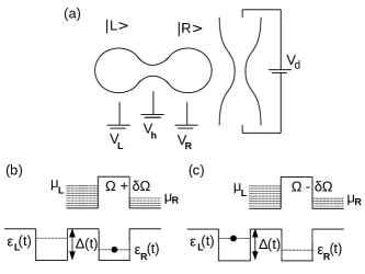
Figure 1: (a) Scheme of a double quantum dot with a nearby QPC measuring its charge states, labeled as $|L\rangle$, $|R\rangle$. (b), (c) Scheme of the detection mechanism. The conductance of the detector is sensitive to the qubit’s occupancy: The tunneling amplitude in the QPC is $\Omega+\delta\Omega$ when the right dot is occupied (b) and $\Omega-\delta\Omega$ when the left dot is occupied (c).

This model has been extensively studied in the literature. Gurvitz:1997 ; Gurvitz:1998 ; Korotkov:1999 ; Korotkov:2001 The current through the detector directly measures the “position” of the electron in the dot. Under the assumptions of uniform tunneling matrix elements, $\delta\Omega_{l,r}\equiv\delta\Omega$, $\Omega_{l,r}\equiv\Omega$, and density of states in the QPC’s reservoirs, $\rho_{L}$, $\rho_{R}$, the average current for an electron being in the left or right dot, reads $\langle I\rangle_{\pm}=eD/2\cdot(1\pm\delta\Omega/\Omega)^{2}$, where $D\equiv TV_{d}/(2\pi)=2\pi\rho_{l}\rho_{r}\Omega^{2}V_{d}$. Throughout the work we set $\hbar=1$. The QPC’s shot noise power $S_{I}=eI(1-T)$ sets the time scale $\tau_{D}\sim S_{I}/(I_{+}-I_{-})^{2}\approx 1/D(\Omega/\delta\Omega)^{2}(1-T)$ needed to distinguish the detector’s signal form the background noise. The weak measurement regime is then identified by measurements of duration $\tau\ll\tau_{D}$, which can be controlled in principle by tuning the system-detector coupling, the duration of the measurement, or the voltage bias across the QPC. The QPC is effectively a detector at finite $V_{d}$ where it leads to a finite signal $\langle I\rangle\propto V_{d}$. In particular, we assume $V_{d}\gg k_{B}T$ (the temperature $T$ is the smallest energy scale throughout the paper) and $V_{d}\gg\rho\Omega^{2}$ as clarified below. In this regime we neglect the extra decoherence effect due to the detector equilibrium backaction, for instance orthogonality catastrophe dephasing. Aleiner:1997 ; Gefen:2012

An important aspect of the model is that the Hamiltonian in Eq. (1) describes the qubit and the detector as a closed quantum system. However, the QPC is continuously converting the information about the state of the system in a classical — macroscopic — information output which is the current. In other words, while Eq. (1) will evolve the detector to a coherent superposition of states with different charges in the reservoirs, the classical knowledge of the current would correspond to a well-defined number of electrons in each reservoir. A solution of this problem, as pointed out in Ref. Korotkov:2001, , consists of introducing a macroscopic pointer which interacts with the detector. The pointer provides in fact an effective description of the various relaxation processes confining the QPC electrons in one of the two QPC reservoirs. The pointer can be modeled to interact instantaneously at certain times, $t_{1},t_{2}\ldots t_{k}\ldots t_{N}$ with $t_{0}=0$ and $t_{N}=\tau$, and reads out the change of the number of electrons in the right reservoir, $\mu_{R}$, as schematically depicted in Fig. 2. At any time $t=t_{k}$ the pointer reads the number of electrons, $m_{k}$, transmitted to the collector within the time interval $\Delta t_{k}=t_{k+1}-t_{k}$, and collapses the qubit-detector system onto a corresponding state depending on the measured value $m_{k}$. Note that the introduction of the pointer results in a new time scale $\Delta t_{k}$ in the problem which is a free parameter in our model. We discuss in the Results section the different regimes corresponding to the relation of this time scale to other time scales in the problem.

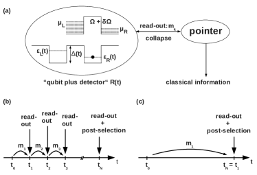
Figure 2: (a) Qubit plus detector interaction with a classical pointer reading out the number $m_{k}$ of electrons having penetrated to the detector’s right reservoir at certain discrete times $t=t_{k}$. Illustration of the continuous readout (b) and coherent (c) measurement regimes, respectively.

The model allows us to include decoherence by considering fluctuations, which naturally arise in the system, of the external parameters, namely the voltage biases $V_{L}$,$V_{R}$, $V_{h}$. In turn they lead to fluctuations of the dots’ parameters, $\epsilon(t)=\epsilon_{0}+\xi(t)\quad$ and $\Delta(t)=\Delta_{0}+\eta(t)$ around their average values $\epsilon_{0}$ and $\Delta_{0}$. Since the explicit relation between $V_{h}$, $V_{L}$, $V_{R}$ and $\epsilon_{0}$, $\Delta_{0}$ depends on microscopic details, we effectively assume here a general linear relation and the effect of decoherence is therefore described by replacing the dot’s Hamiltonian with $H_{0}(t)\rightarrow H_{0}+H_{\xi}(t)$, with

$$H_{0}=\epsilon_{0}\,\sigma_{z}+\Delta_{0}\,\sigma_{x}=\omega\mathbf{m}\cdot\mathbf{\sigma},$$ (6)

$$H_{\xi}(t)=\sum_{i}\,\xi_{i}(t)\,\mathbf{k}_{i}\cdot\mathbf{\sigma}.$$ (7)

Here $\omega=\sqrt{\epsilon_{0}^{2}+\Delta_{0}^{2}}$ is the oscillation frequency of the system and $\mathbf{m}$ defines the corresponding eigenstates. To this regard, the index $i$ labels the different independent decoherence sources, ideally corresponding to the independent voltage sources. For each of them $\mathbf{k}_{i}$ indicates the direction of the fluctuations with $|\mathbf{k}_{i}|=1$ and $\xi_{i}(t)$ is assumed to be a Gaussian white noise, that is,

$$\left\langle\,\xi_{i}(s)\,\right\rangle_{\xi}=0,\quad\left\langle\,\xi_{i}(s_{1})\,\xi_{j}(s_{2})\right\rangle_{\xi}=\gamma_{i}\,\delta(s_{1}-s_{2})\,\delta_{ij}$$ (8)

where $\gamma_{i}$ describes the strength of the correlation function. For the sake of simplicity we present in the following our general results for the case of a single decoherence source. The results in the case of several noise sources are a straightforward extension and are discussed at the end.

Finally, we can include in the model the description of postselection, as required by the WV measurement protocol. As pointed out in Ref. Romito-Gefen-Blanter:2008, , a second QPC strongly measuring the charge on the dot at any time after the weak measurement can effectively realize a postselection in any given qubit state, $|\Psi_{f}\rangle$. Without loss of generality we therefore consider the situation where the postselection takes place immediately after the weak measurement. Within our model the postselection into the state $|\Psi_{f}\rangle$ is described by the action of the corresponding projection operator $\Pi_{f}$ acting at the end of the weak measurement.

III General Expression for the Weak Value in the Presence of Decoherence

The WV protocol we are interested in consists of preparing the double dot in a given initial state $|\Psi(t_{0})\rangle$ at time $t_{0}$, making the system interact with the detector for a time $\tau$, and finally strongly measuring it in the postselected state in $|\Psi_{f}\rangle$. The quantity of interest is the WV of the electron’s occupancy in the double dot, that is, the value of $\sigma_{z}(\tau)$ conditional to a positive postselected outcome, which we denote by ${}_{\Pi_{\textrm{f}}}\langle\sigma_{z}(\tau)\rangle_{\Psi(t_{0})}$. In fact, such a quantity is inferred from the postselected output of the detector, that is, the average current in the QPC conditional to the postselection ${}_{\Pi_{\textrm{f}}}\langle I(\tau)\rangle_{\Psi(t_{0})}=e/\tau\,_{\Pi_{\textrm{f}}}\langle n(\tau)\rangle_{\Psi(t_{0})}$ through

$${}_{\Pi_{\textrm{f}}}\langle\sigma_{z}(\tau)\rangle_{\Psi(t_{0})}=\frac{{}_{\Pi_{\textrm{f}}}\langle I(\tau)\rangle_{\Psi(t_{0})}-eD/2h}{I_{+}-I_{-}}\,.$$ (9)

The average conditional (postselected) value of the number of electrons, ${}_{\Pi_{\textrm{f}}}\langle n(\tau)\rangle_{\Psi(t_{0})}$, having passed through the QPC during the measurement time $\tau$ is

$$\left.\vphantom{\langle\Omega\rangle}\right._{\Pi_{\textrm{f}}}\langle n(\tau)\rangle_{\Psi(t_{0})}=\sum_{\begin{subarray}{c}m\end{subarray}}m\,\left.P(m\,\right|\,\Pi_{f})\,.$$ (10)

In Eq. (10) $m$ indicates the total number of electrons having reached the collector and $P(m\,|\,\Pi_{f})$ is the conditional probability that $m$ electrons have been transmitted through the QPC given that the qubit is finally found to be in a state represented by the projection operator $\Pi_{f}$. Note that Eq. (10) is valid for any strength of the measurement. We keep our analysis valid for a general measurement strength until specified differently.

The conditional probabilities in Eq. (10), can be directly expressed in terms of the total density matrix $R(t)$ of the qubit-detector system. Following the formalism of Gurvitz Gurvitz:1997 and Korotkov, Korotkov:2001 a pure state of the qubit-detector system is described by a wave function $\left|\,\Psi(t)\,\right\rangle=(|\,\Psi^{\uparrow}(t)\,\rangle,|\,\Psi^{\downarrow}(t)\,\rangle)$, where $\sigma=\uparrow,\downarrow$ labels the eigenstates of $\sigma_{z}$ and $|\Psi^{\sigma}(t)\rangle$ is a many-body state of the QPC,

$$\left|\,\Psi^{\sigma}(t)\,\right\rangle =\left(b^{(0)\,\sigma}(t)+\sum_{\begin{subarray}{c}l\leq\mu_{l};r>\mu_{r}\end{subarray}}b^{(1)\,\sigma}_{lr}(t)\,a_{r}^{\dagger}a_{l}\right.$$

$$\left.+\sum_{\begin{subarray}{c}l,l^{\prime}\leq\mu_{l};r,r^{\prime}>\mu_{r}\end{subarray}}b^{(2)\,\sigma}_{ll^{\prime}rr^{\prime}}(t)\,a_{r}^{\dagger}a_{r^{\prime}}^{\dagger}a_{l}a_{l^{\prime}}+\cdots\right)\,|0\rangle\,,$$ (11)

and $|b^{(i)}(t)|^{2}$ describes the probability of finding the entire qubit-detector system in the corresponding state described by the creation and annihilation operators with $l$, $r$ labeling the single particle states in the left, right reservoirs, respectively. The corresponding qubit-detector density matrix $R(t)$ has components

$$R_{\sigma\sigma^{\prime}}(t)=\left(\begin{array}[]{ccccc}R^{(0,0)}_{\sigma\sigma^{\prime}}(t)&R^{(1,0)}_{\sigma\sigma^{\prime}}(t)&\ldots&&\\ R^{(0,1)}_{\sigma\sigma^{\prime}}(t)&R^{(1,1)}_{\sigma\sigma^{\prime}}(t)&\ddots&&\\ \vdots&\vdots&&R^{(m,n)}_{\sigma\sigma^{\prime}}(t)&\ldots\end{array}\right)\,.$$ (12)

Here each entry $R^{(m,n)}_{\sigma\sigma^{\prime}}(t)$ is a matrix whose dimensions are given by the infinitely many states labeled by $l,r,l^{\prime},r^{\prime},l^{\prime\prime},r^{\prime\prime}\ldots l^{(m)},r^{(m)}$ and $l,r,l^{\prime},r^{\prime},l^{\prime\prime},r^{\prime\prime}\ldots l^{(n)},r^{(n)}$. Each of the entries $b_{l_{1}\ldots l_{m}r_{1}\ldots r_{m}}^{(m)\,\sigma}(t)\,\overline{b}_{l_{1}\ldots l_{n}r_{1}\ldots r_{n}}^{(n)\,\sigma^{\prime}}(t)$ (the $\overline{\cdot}$ indicates the complex conjugate) in $R^{(m,n)}_{\sigma\sigma^{\prime}}(t)$ characterizes the coherences between all the possible states with $m$ and $n$ electrons detected in the collector of the QPC at time $t$. In particular, the trace of each diagonal matrix $R^{(m,m)}_{\sigma\sigma^{\prime}}(t)$ identifies the probability that exactly $m$ electrons have passed through the detector until time $t$, namely

$$P(m)=\textrm{tr}_{\textrm{sys}}\left\{\mathcal{R}^{(m)}(t)\right\}=\textrm{tr}_{\textrm{sys}}\left\{\textrm{tr}_{\textrm{det}}\left\{R^{(m,m)}(t)\right\}\right\},$$ (13)

where we introduced the quantity $\mathcal{R}_{\sigma\sigma^{\prime}}^{(m)}(t)=\textrm{tr}_{\textrm{det}}\{R_{\sigma\sigma^{\prime}}^{(m,m)}\}$. Also the reduced density matrix of the dot, $\rho(t)=\textrm{tr}_{\textrm{det}}\left\{R(t)\right\}$, can be written as

$$\rho(t)=\sum_{\begin{subarray}{c}m\end{subarray}}\mathcal{R}^{(m)}=\sum_{\begin{subarray}{c}m\end{subarray}}P(m)\cdot\rho^{(m)}(t)\,,$$ (14)

where $\rho^{(m)}(t)=\mathcal{R}^{(m)}(t)/(\textrm{tr}\left\{\mathcal{R}^{(m)}(t)\right\})$ describes the state of the qubit where $m$ electrons have reached the collector.

Besides the inherent quantum-mechanical fluctuations, the stochastic parameter $\xi(t)$ assumes different values at each replica of the experiment according to its probability distribution. In order to properly take into account the average over fluctuations, we can first rewrite the conditional probability Eq. (10) using Bayes’ theorem as $P(m|\Pi_{f})=P(m)P(\Pi_{f}|m)/\sum_{m}P(\Pi_{f})$. The WV of each run of the experiment is now weighted with the probability of a successful postselection in the corresponding run of the experiment, which also depends on the specific noise realization. This means that the average over the fluctuations $\xi(t)$ in the weak value is properly taken into account by separately averaging over $\xi$ both the conditional average value of $m$ and the postselection probability. Romito:2009 This leads to

$$\left.\vphantom{\langle\Omega\rangle}\right._{\Pi_{\textrm{f}}}\langle n(\tau)\rangle_{\Psi(t_{0})}=\frac{\left\langle\sum_{\begin{subarray}{c}m\end{subarray}}m\,\left.P(\Pi_{f}\,\right|(m|\xi))\,P(m|\xi)\right\rangle_{\xi}}{\left\langle\sum_{\begin{subarray}{c}m\end{subarray}}\left.P(\Pi_{f}\,\right|(m|\xi))\,P(m|\xi)\right\rangle_{\xi}}\vphantom{\frac{\frac{\Omega}{\Omega}}{\frac{\Omega}{\Omega}}}.$$ (15)

Identifying the emerging probabilities in terms of the matrix $\mathcal{R}^{(m)}$ similar to Eq. (13) yields the conditional current

$$\left.\vphantom{\langle\Omega\rangle}\right._{\Pi_{\textrm{f}}}\langle I(\tau)\rangle_{\Psi(t_{0})}=\frac{e}{\tau}\,\frac{\sum_{\begin{subarray}{c}m\end{subarray}}m\,\textrm{tr}\left\{\Pi_{f}\cdot\langle\mathcal{R}^{(m)}(\tau)\rangle_{\xi}\right\}}{\sum_{\begin{subarray}{c}m\end{subarray}}\textrm{tr}\left\{\Pi_{f}\cdot\langle\mathcal{R}^{(m)}(\tau)\rangle_{\xi}\right\}}.$$ (16)

As already pointed out the weak measurement regime is obtained when $(\delta\Omega/\Omega)^{2}\tau\ll 1/D(1-D/V_{d})$. The WV can be identified from the coefficients in the expansion

$$\left.\vphantom{\langle\Omega\rangle}\right._{\Pi_{\textrm{f}}}\langle I(\tau)\rangle_{\Psi(t_{0})}=\langle I(\tau)\rangle+\left.\vphantom{\langle\Omega\rangle}\right._{\Pi_{\textrm{f}}}\langle I(\tau)\rangle^{\textrm{weak}}_{\Psi(t_{0})}\cdot\frac{\delta\Omega}{\Omega}+\mathcal{O}\left(\frac{\delta\Omega^{2}}{\Omega^{2}}\right).$$ (17)

We discuss the validity of this expansion later. From the definition of the weak measurement regime, we expect to be sensitive to coherence effects for time scales $\tau\ll 1/D(1-D/V_{d})(\Omega/\delta\Omega)^{2}$. The WV is completely determined by the knowledge of the probabilities $P(m)$ and the conditional reduced dot’s density matrix $\langle\rho^{(m)}(\tau)\rangle_{\xi}$. Further analysis now focuses on the evaluation of $\langle\mathcal{R}^{(m)}(\tau)\rangle_{\xi}$.

IV System-detector dynamics in presence of decoherence

IV.1 Coherent detection

First we consider the case where a single readout by the external pointer takes place at the end of the measurement process, that is, at $t=\tau$, immediately followed by the postselection. In this case the coherent evolution of the system and detector is not disturbed by the pointer, and we thus name it coherent detection.

The WV is fully determined by the knowledge of the averaged matrices $\langle\mathcal{R}^{(m)}(\tau)\rangle_{\xi}$. We can derive a differential equation for $\langle\mathcal{R}^{(m)}(\tau)\rangle_{\xi}$ starting from the von Neumann equation for the qubit-detector system, $i\partial_{t}R(t)=\left[H(t),R(t)\right]$. After inserting the Hamiltonian in Eq. (1) with the specific choice of a single fluctuation source, that is, $\epsilon(t)=\epsilon_{0}+k_{z}\cdot\xi(t)$, $\Delta(t)=\Delta_{0}+k_{x}\cdot\xi(t)$, one obtains for the qubit-detector evolution

$$\partial_{t}R(t)=-i\,\left[\,M,\,R(t)\,\right]-i\,\xi(t)\,\left[\,N,\,R(t)\,\right]$$ (18)

where $\partial_{t}=\partial/\partial t$. Here,

$$M =\frac{1}{2}\,\Delta\hat{H}^{+}+\Delta\cdot\sigma_{x}+\frac{1}{2}\left(\Delta\hat{H}^{-}+2\,\epsilon_{0}\right)\otimes\sigma_{z}\,,$$

$$N =\vphantom{\frac{1}{2}}\mathbf{\sigma}\cdot\mathbf{k}\,.$$ (19)

Introducing an interaction picture with respect to $M$, which transforms the arbitrary operator $A$ as $A_{I}(t)=e^{-iMt}\cdot A\cdot e^{iMt}$, transfers Eq. (18) into $\partial_{t}R_{I}(t)=-i\,\xi(t)\,\left[\,N_{I}(t),\,R_{I}(t)\,\right]$. Iteratively solving this equation, one obtains after taking the average with respect to $\xi(t)$

$$\left\langle R_{I}(t)\right\rangle_{\xi} =\left\langle R(0)\right\rangle_{\xi}-i\int_{0}^{t}\textrm{d}s_{1}\langle\xi(s_{1})\rangle_{\xi}\,[N_{I}(s_{1}),\left\langle R_{I}(0)\right\rangle_{\xi}]$$

$$+(-i)^{2}\int_{0}^{t}\textrm{d}s_{1}\int_{0}^{s_{1}}\textrm{d}s_{2}\langle\xi(s_{1})\xi(s_{2})\rangle_{\xi}$$

$$\quad\cdot[N_{I}(s_{1}),[N_{I}(s_{2}),\left\langle R_{I}(0)\right\rangle_{\xi}]]$$

$$+(-i)^{3}\int_{0}^{t}\textrm{d}s_{1}\int_{0}^{s_{1}}\textrm{d}s_{2}\int_{0}^{s_{2}}\textrm{d}s_{3}\langle\xi(s_{1})\xi(s_{2})\xi(s_{3})\rangle_{\xi}$$

$$\quad\cdot[N_{I}(s_{1}),[N_{I}(s_{2}),[N_{I}(s_{3}),\left\langle R_{I}(0)\right\rangle_{\xi}]]]$$

$$+\ldots$$ (20)

Due to the $\delta$-like time correlations in Eq. (8), the average can be performed exactly order by order. The so obtained integral equation for $R(t)$ is more conveniently written in a differential form as

$$\partial_{t}\left\langle R(t)\right\rangle_{\xi}=-\,\frac{\gamma}{2}\,\left[\,N,\,\left[N,\,\left\langle R(t)\right\rangle_{\xi}\right]\right]-i\,\left[\,M,\left\langle R(t)\right\rangle_{\xi}\,\right]$$ (21)

The density matrix is expressed as a linear combination of Pauli-matrices of the dot’s space

$$\left\langle R(t)\right\rangle_{\xi}=\frac{1}{2}\,\sum_{j=0}^{3}\hat{v}_{j}(t)\cdot\sigma_{j}.$$ (22)

where each $\hat{v}_{j}(t)$ is a matrix in the QPC Hilbert space with $\textrm{tr}\left\{\hat{v}_{0}(t)\right\}\equiv 1$. Substituting Eq. (22) into the averaged von Neumann equation (21) yields a set of differential equations for $\hat{v}_{j}(t)$ which fully describes the averaged evolution of the qubit-detector system:

$$\dot{\hat{v}}_{0} =-\frac{i}{2}\,\left[\Delta\hat{H}^{-},\hat{v}_{z}(t)\right]-\frac{i}{2}\,\left[\Delta\hat{H}^{+},\hat{v}_{0}(t)\right]$$

$$\dot{\hat{v}}_{x} =2\gamma\left(\vphantom{\int}(k_{x}^{2}-1)\hat{v}_{x}+k_{x}k_{y}\hat{v}_{y}+k_{x}k_{z}\hat{v}_{z}\right)-2\epsilon_{0}\hat{v}_{y}$$

$$\quad-\frac{i}{2}\,\left[\Delta\hat{H}^{+},\hat{v}_{x}\right]-\frac{1}{2}\,\left\{\Delta\hat{H}^{-},\hat{v}_{y}\right\}$$

$$\dot{\hat{v}}_{y} =2\gamma\left(\vphantom{\int}k_{x}k_{y}\hat{v}_{x}+(k_{y}^{2}-1)\hat{v}_{y}+k_{y}k_{z}\hat{v}_{z}\right)+2\epsilon_{0}\hat{v}_{y}$$

$$\quad-2\Delta\hat{v}_{z}-\frac{i}{2}\,\left[\Delta\hat{H}^{+},\hat{v}_{y}\right]+\frac{1}{2}\,\left\{\Delta\hat{H}^{-},\hat{v}_{y}\right\}$$

$$\dot{\hat{v}}_{z} =2\gamma\left(\vphantom{\int}k_{x}k_{z}\hat{v}_{x}+k_{y}k_{z}\hat{v}_{y}+(k_{z}^{2}-1)\hat{v}_{z}\right)+2\Delta\hat{v}_{y}$$

$$\quad-\frac{i}{2}\,\left[\Delta\hat{H}^{-},\hat{v}_{0}\right]-\frac{i}{2}\,\left[\Delta\hat{H}^{+},\hat{v}_{z}\right].$$ (23)

Equations. (23) describe a set of infinitely many coupled differential equations. They are a generalization to a density matrix of the results obtained in Ref. Gurvitz:1997, for the simple case of a pure state. Note that such a generalization is essential in our case to properly treat fluctuations of $\xi$. One may further note that the fluctuations treated here differ from Ref. Korotkov:2001, , where the system’s evolution for a given stochastic measurement output $I(t)$ is studied. Considering the matrix elements of $R(t)$ between two sectors $(m,n)$ with $m$ and $n$ electrons having passed through the QPC, we trace out the QPC degrees of freedom to obtain a differential equation for

$$\langle\mathcal{R}^{(m)}(t)\rangle_{\xi}=\frac{1}{2}\,\left(\mathbf{v}^{(m)}(t)\cdot\mathbf{\sigma}\right)\,,$$ (24)

where $v_{j}^{(m)}(t)=\textrm{tr}_{\textrm{det}}\{\hat{v}_{j}^{(m,m)}(t)\}$. The details of the calculation are presented in appendix A. Here we report the resulting differential equation, which can be recast as a differential equation for $v_{j}^{(m)}(t)$, that is,

$$\partial_{t}\,\mathbf{v}^{(n)}(t)=\left(G_{0}+G_{\mathbf{k}}+G_{1}\right)\cdot\mathbf{v}^{(n)}(t)+G_{2}\cdot\mathbf{v}^{(n-1)}(t)\,,$$ (25)

with

$$G_{0}=\left(\begin{array}[]{cccc}\,\,0&0&0&0\\ \,\,0&0&-2\,\epsilon_{0}&0\\ \,\,0&2\,\epsilon_{0}&0&-\,2\,\Delta_{0}\\ \,\,0&0&2\,\Delta_{0}&0\end{array}\right),$$

$$G_{\mathbf{k}}=2\,\gamma\,\left(\begin{array}[]{cccc}\,\,0&0&0&0\\ \,\,0&k_{x}^{2}-1&k_{x}\,k_{y}&k_{x}\,k_{z}\\ \,\,0&k_{x}\,k_{y}&k_{y}^{2}-1&k_{y}\,k_{z}\\ \,\,0&k_{x}\,k_{z}&k_{y}\,k_{z}&k_{z}^{2}-1\end{array}\right),$$

$$G_{1}=-\,\frac{D}{2}\left(\begin{array}[]{cccc}1+\frac{\delta\Omega^{2}}{\Omega^{2}}&0&0&2\,\frac{\delta\Omega}{\Omega}\\ 0&1+\frac{\delta\Omega^{2}}{\Omega^{2}}&0&0\\ 0&0&1+\frac{\delta\Omega^{2}}{\Omega^{2}}&0\\ 2\,\frac{\delta\Omega}{\Omega}&0&0&1+\frac{\delta\Omega^{2}}{\Omega^{2}}\end{array}\right),$$

$$G_{2}=\frac{D}{2}\left(\begin{array}[]{cccc}1+\frac{\delta\Omega^{2}}{\Omega^{2}}&0&0&2\,\frac{\delta\Omega}{\Omega}\\ 0&1-\frac{\delta\Omega^{2}}{\Omega^{2}}&0&0\\ 0&0&1-\frac{\delta\Omega^{2}}{\Omega^{2}}&0\\ 2\,\frac{\delta\Omega}{\Omega}&0&0&1+\frac{\delta\Omega^{2}}{\Omega^{2}}\end{array}\right).$$

The above equation is obtained to lowest order in $\rho\Omega^{2}\ll V_{d}$, under the assumptions that: (i) the detector’s transition amplitude only weakly depends on the energies, that is, $\Omega_{lr}\equiv\Omega$; (ii) the densities of states in the QPC’s collectors are constant, $\rho_{l}(E_{l_{k}})\equiv\rho_{l}$ and $\rho_{r}(E_{r_{k}})\equiv\rho_{r}$; (iii) at $t=0$ the energy levels of the detector are filled up to the Fermi-level so that $m=0$, that is, $\mathbf{v}^{(n)}(0)=(1,v_{x},v_{y},v_{z})\cdot\delta_{n,0}$. As evident in Eq. (25), for $D\rightarrow 0$ or $\delta\Omega\rightarrow 0$, respectively, the system evolves undisturbed, while for $\gamma\rightarrow 0$ our result reduces to that in Ref. Gurvitz:1997, .

According to Eqs. (16) and (17) we can obtain the expression for the WV by solving the differential equations (25) perturbatively in the regime $\delta\Omega\ll\Omega$. The details of the derivation are given in Appendix B. We highlight here that the perturbative solution is a valid approximation for $\tau\ll 1/D(\Omega/\delta\Omega)^{2}$ exactly corresponding to the weak measurement regime. This finally yields the expression for the WV

$$\left.\vphantom{\langle\Omega\rangle}\right._{\Pi_{\textrm{f}}}\langle I(\tau)\rangle^{\textrm{weak}}_{\Psi(t_{0})}=e\,D\,\frac{\frac{1}{\tau}\,\intop_{0}^{\tau}\textrm{d}s\,v_{z}(s)+\frac{1}{\tau}\,\intop_{0}^{\tau}\textrm{d}s\,n_{z}(s)}{\mathbf{n}\cdot\mathbf{v}(\tau)}.$$ (26)

Here $\tau$ is the duration time of the weak measurement and we effectively introduced a time dependence in the postselection operator $\Pi_{f}(\tau)=1/2\,(\mathbf{n}(\tau)\cdot\mathbf{\sigma})$, $\mathbf{n}=\mathbf{n}(\tau)$ is then the postselected state at time $t=\tau$ instantaneously after the measurement. In the notation in Eq. (26), $\mathbf{v}(s)$ is defined by $\mathbf{v}(s)=\exp\left[\left(G_{0}+G_{\mathbf{k}}\right)s\right]\cdot\mathbf{v}(0)$, while $\mathbf{n}(s)=\exp\left[\left(-G_{0}+G_{\mathbf{k}}\right)s\right]\cdot\mathbf{n}(0)$.

The result in Eq. (26) is already captured by a minimal model where the coupling to the detector is described by a von Neumann Hamiltonian Neumann $H_{\textrm{int}}(t)=\lambda g(t)\,\hat{p}\,\sigma_{z}$. It linearly couples the measured observable $\sigma_{z}$ to a detector’s variable $\hat{p}$, $\lambda$ indicates the coupling constant and the time dependency of the interaction is included in the function $g(t)$. The WV of $\sigma_{z}$ is inferred from the conditional value of the conjugate variable $\hat{q}$,

$$\left.\vphantom{\langle\Omega\rangle}\right._{\Pi_{\textrm{f}}}\langle\hat{q}(\tau)\rangle^{\textrm{weak}}_{\Psi(t_{0})}=\lambda\,\textrm{Re}\int_{0}^{\tau}\textrm{d}s\,\frac{\langle\Pi_{f}(\tau)\,\sigma_{z}(s)\rangle}{\langle\Pi_{f}(\tau)\rangle}$$ (27)

obtained to leading order in the coupling. The effect of decoherence is included in the correlation function $\langle\Pi_{f}(\tau)\,\sigma_{z}(s)\rangle$ resulting in Eq. (26). Equation (27) elucidates the role of coherent system evolution between the measurement at time $s$ and the postselection at time $\tau$.

IV.2 Continuous readout

Opposed to a coherent detection, the regime of continuous readout is characterized by the detector’s state being frequently read out by the pointer. This limit is described by a sequence of readouts at times $t=t_{k}$, $k=1\ldots N$, where the time interval between readouts $\Delta t_{k}:=t_{k+1}-t_{k}\equiv\Delta t$ is the shortest time scale in the problem, that is, $\Delta t\ll\textrm{min}\{1/\omega,1/\gamma,1/D\}$. The conditional number of transmitted electrons Eq. (16) can now be expressed as the sum over all permutations describing quantum jumps at all possible times

$$\left.\vphantom{\langle\Omega\rangle}\right._{\Pi_{\textrm{f}}}\langle n(\tau)\rangle_{\Psi(t_{0})}=\\ \frac{\sum\limits_{\sum_{j}m_{j}=m}m\,\textrm{tr}\left\{\Pi_{f}\cdot\langle\mathcal{R}^{(m_{1},\ldots,m_{N})}(\tau)\rangle_{\xi}\right\}}{\sum\limits_{\sum_{j}m_{j}=m}\textrm{tr}\left\{\Pi_{f}\cdot\langle\mathcal{R}^{(m_{1},\ldots,m_{N})}(\tau)\rangle_{\xi}\right\}}.$$ (28)

where $j=1\ldots N$ and $\mathcal{R}^{(m_{1},\ldots,m_{N})}(\tau)$ characterizes the qubit’s density matrix weighted with the probability that exactly $m_{k}$ electrons have passed within each time interval $\Delta t_{k}$. Each readout corresponds to a collapse of the qubit-detector system in the sector of $m_{k}$ electrons having passed with the corresponding probability $P(m_{k};t_{k})$.

In the regime $\Delta t\ll\textrm{min}\{1/\omega,1/\gamma,1/D\}$ at most one electron penetrates through the QPC between two subsequent readouts.  The probabilities that either exactly one (quantum jump Korotkov:2001 ; Korotkov_Averin:2001 ) or zero electrons accumulate in the collector within a readout period time are computed in appendix C. They are given by $P(0;\Delta t)=\{A\cdot\mathbf{v}^{(n_{k})}(t_{k})\}_{0}$ and $P(1;\Delta t)=\{B\cdot\mathbf{v}^{(n_{k})}(t_{k})\}_{0}$, respectively, where the index $\{\ldots\}_{0}$ denotes the zeroth component and

$$A ={1}_{(4)}+\left(G_{0}+G_{\mathbf{k}}+G_{1}\right)\,\Delta t+\mathcal{O}\left(\Delta t^{2}\right)$$

$$B =G_{2}\Delta t+\mathcal{O}\left(\Delta t^{2}\right).$$ (29)

$\mathcal{O}(\Delta t^{2})$ indicates higher order terms for $\Delta t\ll\textrm{min}\{1/\omega,1/\gamma,1/D\}$. In the limit of $N\rightarrow\infty$, $\Delta t\rightarrow 0$ while keeping $N\cdot\Delta t=\tau$ constant, the conditional number of transferred electrons in Eq. (28) can be analytically evaluated (cf. appendix C), yielding the exact result

$$\left.\vphantom{\langle\Omega\rangle}\right._{\Pi_{\textrm{f}}}\langle n(\tau)\rangle_{\Psi(t_{0})}=\tau\,\frac{\mathbf{n}\cdot G_{2}\cdot e^{(G_{0}+G_{\mathbf{k}}+G_{1}+G_{2})\,\tau}\cdot\mathbf{v}(0)}{\mathbf{n}\cdot e^{(G_{0}+G_{\mathbf{k}}+G_{1}+G_{2})\,\tau}\cdot\mathbf{v}(0)}.$$ (30)

The WV can be easily extracted by ${}_{\Pi_{\textrm{f}}}\langle I(\tau)\rangle^{\textrm{weak}}_{\Psi(t_{0})}=\lim_{\delta\Omega/\Omega\to 0}(_{\Pi_{\textrm{f}}}\langle I(\tau)\rangle_{\Psi(t_{0})})$, where

$$\left.\vphantom{\langle\Omega\rangle}\right._{\Pi_{\textrm{f}}}\langle I(\tau)\rangle_{\Psi(t_{0})}^{\textrm{weak}}=\frac{e\Omega}{\delta\Omega}\left(\frac{1}{\tau}\cdot\vphantom{\rangle}_{\Pi_{\textrm{f}}}\langle n(\tau)\rangle_{\Psi(t_{0})}-\frac{D}{2}\right)+\mathcal{O}\left(\frac{\delta\Omega^{2}}{\Omega^{2}}\right)$$ (31)

The simultaneous presence of $G_{1}+G_{2}$ and $G_{\mathbf{k}}$ in Eq. (30) defines a new time scale $1/\gamma\simeq 1/D(\Omega/\delta\Omega)$ which describes the extra source of decoherence emerging from the detector itself. Note also that Eqs. (30) and (31) are valid at any time. The derivation indeed relies on the perturbative solution in Appendix B, which is valid in the limit $\Delta t\to 0$; hence, the exact composition of subsequent evolution between different readouts holds at any time.

V Results

Equations. (26), (30) and (31) represent the main results of our paper. They express the WVs in the two limiting cases of coherent detection and continuous readout in terms of the system dynamics. Generally, they give rise to four different time scales, which characterize (i) the system’s dynamics, $1/\omega$, (ii) the decoherence, $1/\gamma$, (iii) the detector dynamics, $1/D$, and (iv) the backaction, $1/D\cdot(\Omega/\delta\Omega)^{2}$. We realistically assume $1/D$ to be the shortest time scale in our problem and focus on $\tau\gg 1/D$. The effects of the detector at this time scale dominated by the Zeno effect, Gurvitz:2008 though inherent in Eq. (25), do not play a significant role at the larger time scales of interest where decoherence takes place. Consistently with our perturbative analysis, we further consider $\tau\ll 1/D\cdot(\Omega/\delta\Omega)^{2}$.

The WV can be visualized via the motion of $\mathbf{v}(t)$ and $\mathbf{n}(t)$ on the Bloch-sphere for $\mathbf{v}=(v_{x},v_{y},v_{z})$ and $\mathbf{n}=(n_{x},n_{y},n_{z})$, as depicted in Fig. 3. $|\mathbf{v}(t)|\leq 1$ characterizes the coherence of the qubit’s state, which is initially prepared in a pure quantum state with $|\mathbf{v}(t=0)|=1$.

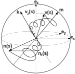
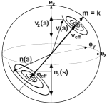
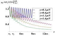
Figure 3: Schematic evolution of $\mathbf{v}(s)$ and $\mathbf{n}(s)$ on the Bloch-sphere for (a) $\mathbf{m}\neq\mathbf{k}$ and (b) $\mathbf{m}=\mathbf{k}$. (c) WV as a function of $\tau$ for different $\gamma$; (d) WV for different $\gamma$ at $\tau_{1}=0.10\,\textrm{ns}$ and $\tau_{2}=1.31\,\textrm{ns}$, marked in panel (c). In all plots the parameters are chosen as $\epsilon_{0}=20\,\mu\textrm{eV}$, $\Delta_{0}=3\,\mu\textrm{eV}$, $\mathbf{k}\approx-0.89\,\mathbf{e}_{x}+0.45\,\mathbf{e}_{z}$, $\mathbf{v}(0)=(0.5,-0.33,0.80)$ and $\mathbf{n}=(-0.20,0.75,0.63)$.

We start with analyzing the case of coherent detection, that is, the dynamical evolution obtained in Eq. (26). In this regime the effect of decoherence essentially reduces to the dynamics of the qubit alone in the presence of decoherence. Accordingly, the WV presents different behaviors in different regimes defined by the durations of the measurement, $\tau$, compared to the remaining time scales $1/\omega$, $1/\gamma$.

For long measurement durations $\tau\gg 1/\gamma$, the qubit’s state generally relaxes towards a fully statistical mixture, $\mathbf{v}(t)=0$, as shown in Fig. 3(c), except for the special case $\vec{k}\parallel\vec{m}$, which is discussed later. Consequently, at time scales where decoherence effects come to play we obtain $\textrm{max}|\left.\vphantom{\langle\Omega\rangle}\right._{\Pi_{\textrm{f}}}\langle I(\tau)\rangle^{\textrm{weak}}_{\Psi(t_{0})}|\leq eD$ and, hence, the peculiar characteristics of WVs are washed out.

For measurements shorter than the decoherence time, the results depend on the system’s evolution time scale. For short measurements, $\tau\ll 1/\omega$, which correspond to negligible dynamics and fluctuations, the vectors $\mathbf{v}(s)$ and $\mathbf{n}(s)$ in Eq. (26) are constant so that a measurement of the averaged detector’s response trivially reflects the WV of the observable $\hat{\sigma}_{z}$ independent from the measurement duration time $\tau$, $\left.\vphantom{\langle\Omega\rangle}\right._{\Pi_{\textrm{f}}}\langle\sigma_{z}(\tau\rightarrow 0)\rangle^{\textrm{weak}}_{\Psi(t_{0})}=\textrm{Re}(\,\left\langle\,\textrm{f}\,\right|\hat{\sigma}_{z}\left|\Psi\right\rangle/\left\langle\,\textrm{f}\,\right|\left.\Psi\right\rangle\,)$.

The system’s dynamics for intermediate durations of the measurement, $\tau\gg 1/\omega$, however, are appreciable. Here, both vectors $\mathbf{n}(s)$ and $\mathbf{v}(s)$ precess about the eigenvector $\mathbf{m}$ of $G_{0}$ with a frequency of $2\,\omega$. Note that, due to its backward-in-time evolution, $\mathbf{n}(s)$ precesses in the opposite direction as compared to $\mathbf{v}(s)$. Due to the oscillatory dependence of the denominator in Eq. (26), peculiar WVs may occur for properly fine-tuned measurement duration times. WVs much larger than $1$ are realized, for instance, for orthogonal states when $|1+\mathbf{n}\cdot\mathbf{v}(\tau)|\gg 1$, which leads to $\tau=n\cdot\frac{\pi}{\omega}\pm\Delta\tau$, with $\Delta\tau\ll\frac{1}{|\sin^{2}\alpha|}\,\frac{1}{2\,\omega}$, where $\alpha$ denotes the altitude angle between $\mathbf{v}(0)$ and $\mathbf{m}$. The effect of the strength of the fluctuations on short and intermediate measurements is shown in Figs. 3(c) and 3(d), resulting in a trivial decay towards the steady-state value.

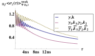
Figure 4: WV as a function of $\tau$ for (a) different $\mathbf{k}$ ($\theta=0$ corresponds to $\mathbf{k}\parallel\mathbf{m}$) and (b) different $\mathbf{n}$ ($\phi=0$ corresponds to $\mathbf{n}\parallel\mathbf{m}$). (c) Same as in (a) in the presence of multiple decoherence sources, where $\gamma=1.0\,\mu\textrm{eV}$, $\mathbf{k}=\frac{1}{\sqrt{2}}\,\mathbf{e}_{x}+\frac{1}{\sqrt{2}}\,\mathbf{e}_{z}$, $\mathbf{k}_{1}=\frac{1}{\sqrt{2}}\,\mathbf{e}_{x}$, $\mathbf{k}_{2}=\frac{1}{\sqrt{2}}\,\mathbf{e}_{z}$, $\gamma_{1}=\frac{1}{\sqrt{2}}\,\mu\textrm{eV}$ $\gamma_{2}=\frac{1}{\sqrt{2}}\,\mu\textrm{eV}$, $\overline{\mathbf{k}}_{1}=\mathbf{m}$, $\overline{\mathbf{k}}_{2}=\mathbf{m}_{\perp}$, $\overline{\gamma}_{1}=(\mathbf{k}\cdot\mathbf{m})\,\mu\textrm{eV}$, $\overline{\gamma}_{2}=(\mathbf{k}\cdot\mathbf{m}_{\perp})\,\mu\textrm{eV}$; all the other parameters are as in Fig. 3.

As already anticipated, an important role is played by the “direction” of the noise term. Its effect is illustrated in Fig. 4(a). As long as $\mathbf{k}$ becomes more and more parallel to the $\mathbf{m}$, the relaxation time toward the steady state becomes longer. In the limiting case, it relaxes to a partially coherent state. The direction of the postselection orientation plays a similar role, as shown in Fig. 4(b). We also note that, in the presence of multiple decoherence sources, even for a given effective direction and strength of the fluctuating term, the decay of the WV still strongly depends on the relative directions between different sources [cf. Fig. 4(c)].

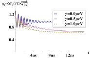
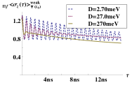
Figure 5: WV for continuous detection for (a) different $\gamma$ with $D=0.270\,\textrm{eV}$ and (b) different $D$ with $\gamma=0.1\,\mu\textrm{eV}$, other parameters as in Fig. 3; in all plots $\delta\Omega/\Omega=0.001$.

The case of a continuous readout is characterized by a rather different behavior. While in both, the coherent and continuous readout regimes, a significant strong decoherence destroys the peculiarities of WVs [cf. Fig. 5(a)], in the latter the detector itself introduces decoherence on the time scale of its backaction. This is visualized in Fig. 5(b). It also shows that $D$ effects the results at the time scales $\tau\ll 1/D(\Omega/\delta\Omega)^{2}$ relevant for WVs, in contrast to the coherent case. The difference between the two cases is highlighted in Fig. 6, comparing the two regimes for different decoherence strength and postselection. The WV in the continuous case can be enhanced as compared to the coherent measurement, leading to peculiar WVs, where a coherent measurement would not [cf. Figs. 6(c) and (d)]. This effect depends on the chosen postselection [cf. Fig. 6(a) vs. Fig. 6(c); Fig. 6(b) vs. Fig. 6(d)] and is suppressed by decoherence [cf. Fig. 6(c) vs Fig. 6(d)]. We can understand these results by analyzing the asymptotic behavior after decoherence has taken place. Equation (31) gives a WV

$$\left.\vphantom{\langle\Omega\rangle}\right._{\Pi_{\textrm{f}}}\langle\sigma_{z}\rangle^{\textrm{weak}}_{\Psi(t_{0})}=\frac{\textrm{tr}\{(1+\mathbf{n}\cdot\mathbf{\sigma})\,\sigma_{z}(s)\,\rho\}}{\textrm{tr}\{(1+\mathbf{n}\cdot\mathbf{\sigma})\,\rho\}}=n_{z}$$ (32)

for a fully incoherent state $\rho\propto 1$. This is the WV of an incoherent state. Romito-Gefen-Blanter:2008 The results from Eq. (26) for the coherent case lead instead to ${}_{\Pi_{\textrm{f}}}\langle\sigma_{z}\rangle^{\textrm{weak}}_{\Psi(t_{0})}=0$ for $\rho\propto 1$. This difference arises because of the coherent evolution in the correlation between measurement and postselection [cf. Eq. (27)] which does not take place in the continuous readout due to the frequent “pointer“ readout. The different steady states are shown in Fig. 6. Though the steady states correspond to times beyond the weak measurement regimes, their difference reflects at shorter time scales as well. There it leads to enhanced WVs exceeding the strong boundary in one case and not in the other (cf. Fig. 6(c) and 6(d)). This explains the sensitivity of the effect to postselection (that counts the steady state of the continuous case) and to decoherence (that suppresses faster peculiar WVs within the standard range in both cases).

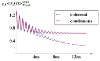
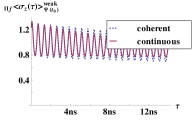
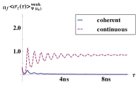
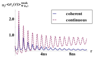
Figure 6: Weak value for continuous detection and coherent readout for different $\gamma$ and pre- and postselection states $\mathbf{n}$, $\mathbf{v}$; $\gamma=1.0\,\mu\textrm{eV}$ in (a), (c) and $\gamma=0.1\,\mu\textrm{eV}$ in (b), (d); $\mathbf{v}(0)=(0.5,-0.33,0.80)$, $\mathbf{n}=(-0.20,0.75,0.63)$ in (a,b) and $\mathbf{v}(0)=(-0.5,0.33,-0.80)$, $\mathbf{n}=(0.50,0.20,0.84)$ in (c), (d). In all plots $D=0.270\,\textrm{eV}$, $\delta\Omega/\Omega=0.001$ and the other parameters as in Fig. 3.

The perturbative solution of the system’s dynamics underlying the result of the coherent detection allows us to discuss, to some extent, the validity of the WV expression in Eq.( 26). As a first check we can require that the second-order contribution is irrelevant compared to the first-order contribution discussed so far, that is, $|\left.\vphantom{\langle\Omega\rangle}\right._{\Pi_{\textrm{f}}}\langle I(\tau)\rangle^{\textrm{weak(2)}}_{\Psi(t_{0})}|\cdot\delta\Omega^{2}/\Omega^{2}\ll|\left.\vphantom{\langle\Omega\rangle}\right._{\Pi_{\textrm{f}}}\langle I(\tau)\rangle^{\textrm{weak}}_{\Psi(t_{0})}|\cdot\delta\Omega/\Omega$, leading to the condition

$$\eta(\tau)=\frac{\delta\Omega}{\Omega}\cdot\frac{D\tau}{2}\cdot\left|\frac{v_{x}(\tau)\,n_{x}+v_{y}(\tau)\,n_{y}}{\frac{1}{\tau}\,\intop_{0}^{\tau}\textrm{d}s\,v_{z}(s)+\frac{1}{\tau}\,\intop_{0}^{\tau}\textrm{d}s\,n_{z}(s)}\right|\ll 1\,.$$ (33)

This imposes a restriction on the validity of the WV’s result also within the regime of weak measurement, as shown in Fig. 7. Indeed, for specific qubit’s parameters $\epsilon_{0}$ and $\Delta_{0}$ and particular boundary conditions $v_{z}(0)$ and $n_{z}$, the numerator in Eq. (33) vanishes at finite duration times for $\tau\ll 1/\gamma$ so that the perturbation is valid at discrete times which depend on the chosen parameters (cf. Fig. 7). For $\tau\gg 1/\gamma$, on the contrary, $\eta\propto\tau^{2}\,e^{-c\,\tau}$ where $c>0$ and the perturbation is asymptotically valid unless $\mathbf{k}=\mathbf{m}=\mathbf{e}_{x}$.

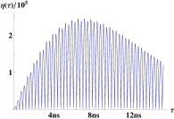
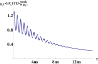
Figure 7: Validity perturbation. (a) Left-hand side of Eq. (33) and (b) the corresponding WV for $\gamma=1.0\,\mu\textrm{eV}$, $D=0.270\,\textrm{eV}$, $\delta\Omega/\Omega=0.001$; all other parameters are as in Fig. 3.

VI Conclusions

In this work we have addressed the effects of decoherence on weak value measurements involving postselection. We have considered the paradigm model of a charge measurement in a double quantum dot by a nearby QPC where we have included fluctuations of the parameters due to external noise sources. After deriving a general expression for the postselected signal (current) in the QPC in terms of the reduced density matrix of the qubit, we have evaluated it explicitly in two different regimes determined by the detector’s readout, namely continuous vs ”single-time“ detector’s readout.

We have characterized the WV’s dependence on the various parameters of the system. In particular, we have shown that statistical fluctuations of the qubit’s parameters generally reduce the WV into the classical range for measurements longer than the decoherence time. On shorter time scales we have determined a boundary for the region of validity of the WV result. Remarkably, there the continuous readout can lead to an enhancement of peculiar weak values as compared to the case of coherent detection.

Appendix A Derivation of Averaged Rate Equations

In this appendix we derive the differential equation (25) out of Eqs. (23) of the main text. In the following, the derivation is presented exemplarily only for $\hat{v}_{x}^{(m)}=\textrm{tr}\{\dot{\hat{v}}_{x}^{(m,m)}(t)\}$ since the other terms ($\hat{v}_{y}^{(m)}$, $\hat{v}_{z}^{(m)}$) are treated completely analogously. It is useful to perfom a ”Laplace” transform for the whole matrices,

$$\hat{v}_{j}^{(m,n)}(E)=\lim_{\delta\to 0}\int\limits_{0}^{\infty}\hat{v}_{j}^{(m,n)}(t)\,\exp\left[i\,(E+i\,\delta)\,t\right]\,\textrm{d}t\,,$$ (A.1)

in order to include the initial conditions of the differential equations that $m=0$ electrons have penetrated through the collector at $t=0$ and, hence, the qubit-detector system is in a pure state. Here, $\delta>0$ ensures the convergence of the integral. A high-energy cutoff is introduced concerning the inverse transform, so that the upper limit of the integral in the inverse transform is $\Lambda\rightarrow\infty$

We can write the differential equations for the Laplace transformed components, $\dot{\hat{v}}_{j}^{(m,m)}(t)$. In this regard, the matrix products in Eq. (23) can be easily calculated by evaluating each $(m,n)$ block as introduced in Eq. (12). Due to the fact that the definition of $\Delta\hat{H}^{+}$ includes terms proportional to $a_{r}^{\dagger}\,a_{r}$ and $a_{l}^{\dagger}\,a_{l}$, diagonal blocks of $\Delta\hat{H}^{+}$ are nonzero, whereas the diagonal blocks $\Delta\hat{H}^{-\,(m,m)}$ vanish. Moreover, since $\Delta\hat{H}^{\pm}$ consists of combinations $a_{l}^{\dagger}\,a_{r}+\textrm{h.c.}$ which raise or lower, respectively, the number of electrons in the detector by exactly one electron, only the off-diagonal blocks $\Delta\hat{H}^{\pm\,(m,m+1)}$ and $\Delta\hat{H}^{\pm\,(m+1,m)}$ neighboring the diagonal blocks are nonzero. Consequently, a blockwise evaluation of the matrix products can be written as

$$\left(\hat{v}_{j}\cdot\Delta\hat{H}^{-}\right)^{(m,n)} =\hat{v}_{j}^{(m,n-1)}\cdot\Delta\hat{H}^{-\,(n-1,n)}+\hat{v}_{j}^{(m,n+1)}\cdot\Delta\hat{H}^{-\,(n+1,n)}\,,$$ (A.2)

$$\left(\hat{v}_{j}\cdot\Delta\hat{H}^{+}\right)^{(m,n)} =\hat{v}_{j}^{(m,n-1)}\cdot\Delta\hat{H}^{+\,(n-1,n)}+\hat{v}_{j}^{(m,n)}\cdot\Delta\hat{H}^{+\,(n,n)}+\hat{v}_{j}^{(m,n+1)}\cdot\Delta\hat{H}^{+\,(n+1,n)}\,,$$ (A.3)

and analogous for $(\Delta\hat{H}^{+/-}\cdot\hat{v}_{j})^{(m,n)}$. Note that $\hat{v}_{j}^{(m,k)}\cdot\Delta\hat{H}^{-\,(k,n)}$ still describes a product of matrices which are of infinite dimension. Thus, applying the ”Laplace” transform to Eqs. (23) for $j=x$ by considering exemplarily $\mathbf{k}=\mathbf{e}_{z}$ leads to

tr $$\left\{\dot{\hat{v}}_{x}^{(m,m)}(t)\right\}=-\pounds^{-1}\left[\textrm{tr}\left\{(i\,E-\delta)\,\hat{v}_{x}^{(m,m)}(E)+\hat{v}_{x}^{(m,m)}(0)\right\}\right]\vphantom{\left[\textrm{tr}\left\{\underbrace{-2\,\gamma\,\hat{v}_{x}^{(m,m)}(E)}_{{A}}\right]\right\}}$$

$$=\pounds^{-1}\left[\textrm{tr}\left\{\underbrace{-2\,\gamma\,\hat{v}_{x}^{(m,m)}(E)}_{=\hat{v}_{a}(E)}\underbrace{-\,2\,\epsilon_{0}\,\hat{v}_{y}^{(m,m)}(E)}_{=\hat{v}_{b}(E)}\right.\right.$$

$$\quad-\,\frac{i}{2}\,\left(\underbrace{\Delta\hat{H}^{+\,(m,m-1)}\cdot\hat{v}_{x}^{(m-1,m)}(E)}_{=\hat{v}_{c}(E)}+\underbrace{\Delta\hat{H}^{+\,(m,m)}\cdot\hat{v}_{x}^{(m,m)}(E)}_{=\hat{v}_{d}(E)}+\underbrace{\Delta\hat{H}^{+\,(m,m+1)}\cdot\hat{v}_{x}^{(m+1,m)}(E)}_{=\hat{v}_{e}(E)}\right)$$

$$\quad+\,\frac{i}{2}\,\left(\underbrace{\hat{v}_{x}^{(m,m-1)}(E)\cdot\Delta\hat{H}^{+\,(m-1,m)}}_{=\hat{v}_{f}(E)}+\underbrace{\hat{v}_{x}^{(m,m)}(E)\cdot\Delta\hat{H}^{+\,(m,m)}}_{=\hat{v}_{g}(E)}+\underbrace{\hat{v}_{x}^{(m,m+1)}(E)\cdot\Delta\hat{H}^{+\,(m+1,m)}}_{=\hat{v}_{h}(E)}\right)$$

$$\quad-\,\frac{1}{2}\,\left(\underbrace{\Delta\hat{H}^{-\,(m,m-1)}\cdot\hat{v}_{y}^{(m-1,m)}(E)}_{=\hat{v}_{i}(E)}+\underbrace{\Delta\hat{H}^{-\,(m,m+1)}\cdot\hat{v}_{y}^{(m+1,m)}(E)}_{=\hat{v}_{j}(E)}\right.$$

$$\quad\quad+\left.\left.\left.\underbrace{\hat{v}_{y}^{(m,m-1)}(E)\cdot\Delta\hat{H}^{-\,(m-1,m)}}_{=\hat{v}_{k}(E)}+\underbrace{\hat{v}_{y}^{(m,m+1)}(E)\cdot\Delta\hat{H}^{-\,(m+1,m)}}_{=\hat{v}_{l}(E)}\right)\right\}\right]\,,$$ (A.4)

where $\pounds^{-1}$ denotes the inverse “Laplace“ transform. We analyze the various terms separately. We start with observing that $\pounds^{-1}[\hat{v}_{a}(E)]=-2\,\gamma\,\textrm{tr}\{\hat{v}_{x}^{(m,m)}(t)\}$ and $\pounds^{-1}[\hat{v}_{b}(E)]=-2\,\epsilon_{0}\,\textrm{tr}\{\hat{v}_{y}^{(m,m)}(t)\}$. Moreover, due to the cyclic invariance of the trace $\pounds^{-1}[\hat{v}_{d}(E)]+\pounds^{-1}[\hat{v}_{g}(E)]=0$. Employing the explicit expression of $\Delta\hat{H}^{\pm}$, reduces the evaluation of the remaining terms to the calculation of

$$\left(\Delta\hat{H}^{+\,(m,m+1)}\right.\left.\cdot\hat{v}_{j}^{(m+1,n)}\right)_{(l_{1}r_{1}\ldots l_{m}r_{m});(l^{\prime}_{1}r^{\prime}_{1}\ldots l^{\prime}_{n}r^{\prime}_{n})}=\sum_{\begin{subarray}{c}l_{m+1}r_{m+1}\end{subarray}}(-1)^{m}2\,\Omega_{l_{m+1}r_{m+1}}\cdot\left(\hat{v}_{j}^{(m+1,m)}\right)_{(l_{1}r_{1}\ldots l_{m}r_{m}l_{m+1}r_{m+1});(l^{\prime}_{1}r^{\prime}_{1}\ldots l^{\prime}_{n}r^{\prime}_{n})}$$ (A.5)

and

$$\left(\Delta\hat{H}^{+\,(m,m-1)}\right.\left.\cdot\hat{v}_{j}^{(m-1,n)}\right)_{(l_{1}r_{1}\ldots l_{m}r_{m});(l^{\prime}_{1}r^{\prime}_{1}\ldots l^{\prime}_{n}r^{\prime}_{n})} =-\,2\,\Omega_{l_{1}r_{1}}\cdot\left(\hat{v}_{j}^{(m-1,m)}\right)_{(l_{2}r_{2}\ldots l_{m}r_{m});(l^{\prime}_{1}r^{\prime}_{1}\ldots l^{\prime}_{n}r^{\prime}_{n})}$$

$$\quad+\,2\,\Omega_{l_{2}r_{2}}\cdot\left(\hat{v}_{j}^{(m-1,m)}\right)_{(l_{1}r_{1}l_{3}r_{3}\ldots l_{m}r_{m});(l^{\prime}_{1}r^{\prime}_{1}\ldots l^{\prime}_{n}r^{\prime}_{n})}$$

$$\quad-\,2\,\Omega_{l_{3}r_{3}}\cdot\left(\hat{v}_{j}^{(m-1,m)}\right)_{(l_{1}r_{1}l_{2}r_{2}l_{4}r_{4}\ldots l_{m}r_{m});(l^{\prime}_{1}r^{\prime}_{1}\ldots l^{\prime}_{n}r^{\prime}_{n})}$$

$$\quad\,\ldots$$

$$\quad+(-1)^{m}\,2\,\Omega_{l_{m}r_{m}}\cdot\left(\hat{v}_{j}^{(m-1,m)}\right)_{(l_{1}r_{1}\ldots l_{m-1}r_{m-1});(l^{\prime}_{1}r^{\prime}_{1}\ldots l^{\prime}_{n}r^{\prime}_{n})}$$ (A.6)

for products concerning the off-diagonal boxes and

$$\left(\Delta\hat{H}^{+\,(m,m)}\right. \left.\cdot\hat{v}_{j}^{(m,n)}\right)_{(l_{1}r_{1}\ldots l_{m}r_{m});(l^{\prime}_{1}r^{\prime}_{1}\ldots l^{\prime}_{n}r^{\prime}_{n})}=2\,\left(E_{r_{1}}+\ldots+E_{r_{m}}-E_{l_{1}}-\ldots-E_{l_{m}}\right)\cdot\left(\hat{v}_{j}^{(m,n)}\right)_{(l_{1}r_{1}\ldots l_{m}r_{m});(l^{\prime}_{1}r^{\prime}_{1}\ldots l^{\prime}_{n}r^{\prime}_{n})}$$ (A.7)

for products with non-zero matrices on the diagonal $(m,m)$. Here, the indices $(l_{1}r_{1}\ldots l_{m}r_{m});(l^{\prime}_{1}r^{\prime}_{1}\ldots l^{\prime}_{n}r^{\prime}_{n})$ precisely determine the scalar entries of the matrices. The analogous multiplications involving $\Delta\hat{H}^{-}$ are evaluated by replacing $\Omega\rightarrow\delta\Omega$. In principle, these products are not restricted to the usage of $\hat{v}_{j}(t)$ and, thus, are valid for a generic matrix of the dimension of $\hat{v}_{j}^{(m\pm 1,m)}$. It is sufficient to consider products where $\Delta\hat{H}^{\pm}$ is on the left, since in the end we need to evaluate the traces and all products can always be arranged such that $\Delta\hat{H}^{\pm}$ is on the left by relying on the cyclic invariance of the traces.

To lowest order in $\rho\,\Omega^{2}\ll V_{d}$, we find that

$$\Omega^{2}\,\sum_{\begin{subarray}{c}l_{k}r_{k}\end{subarray}}\frac{\left(\hat{v}_{j}^{(m,n)}\right)_{(l_{1}r_{1}\ldots l_{k}r_{k}\ldots l_{m}r_{m});(l^{\prime}_{1}r^{\prime}_{1}\ldots l^{\prime}_{n}r^{\prime}_{n})}}{\widetilde{E}+E_{l_{k}}-E_{r_{k}}+i\,\left(\delta+2\,\gamma\right)}\approx 0,\quad\Omega^{2}\,\sum_{\begin{subarray}{c}l^{\prime}_{k}r^{\prime}_{k}\end{subarray}}\frac{\left(\hat{v}_{j}^{(m,n)}\right)_{(l_{1}r_{1}\ldots l_{m}r_{m});(l^{\prime}_{1}r^{\prime}_{1}\ldots l^{\prime}_{k}r^{\prime}_{k}\ldots l^{\prime}_{n}r^{\prime}_{n})}}{\widetilde{E}+E_{l^{\prime}_{k}}-E_{r^{\prime}_{k}}+i\,\left(\delta+2\,\gamma\right)}\approx 0$$ (A.8)

if the sum runs over indices occurring in $\hat{v}_{j}^{(m,m)}(E)$ with the abbreviation $\widetilde{E}=E-E_{l_{1}}-\ldots-E_{l_{k-1}}-E_{l_{k+1}}-\ldots-E_{l_{m}}+E_{r_{1}}+\ldots+E_{r_{k-1}}+E_{r_{k+1}}+\ldots+E_{r_{m}}$. This result holds within the approximation where the energy levels of the detector’s reservoirs are almost continuous so that the sum can be replaced by an integral, that is, $\sum_{\begin{subarray}{c}l_{k}r_{k}\end{subarray}}\rightarrow\int\rho_{l}(E_{l_{k}})\,\rho_{r}(E_{r_{k}})\,\textrm{d}E_{l_{k}}\,\textrm{d}E_{r_{k}}$. Additionally, the hopping amplitudes are assumed to depend weakly on the energy levels, hence, being constant, that is, $\Omega_{lr}\equiv\Omega$, and also the density matrices of the emitter and collector, respectively, are approximated to be constant, with $\rho_{l}(E_{l_{k}})=\rho_{l}$ and $\rho_{r}(E_{r_{k}})=\rho_{r}$. In order to understand that the integral vanishes, it is helpful to realize that the all entries of $\hat{v}_{j}^{(m,n)}$ essentially characterize higher-order retarded Green’s functions which describe the averaged evolution of the density matrix. These Green’s functions have poles in the lower half of the complex plane proportional to $[\widetilde{E}+E_{l_{k}}-E_{r_{k}}+i\,\delta]^{-1}$ which can be shown by iteratively solving the Laplace transformed differential equations (23) for each $\hat{v}_{j}^{(m,n)}(E)$. Thus, a contour integral yields zero since the integrand decreases $\propto\,1/E^{2}$. On the contrary, if the sum does not include a summation over indices of $\hat{v}_{j}^{(m,n)}(E)$, it can be calculated within the same approximation as being

$$\Omega^{2}\,\sum_{\begin{subarray}{c}l_{k}r_{k}\end{subarray}}\frac{1}{\widetilde{E}+E_{l_{k}}-E_{r_{k}}+i\,\left(\delta+2\,\gamma\right)}\approx-i\,\pi\,\rho_{l}\,\rho_{r}\,\Omega^{2}\,\left(V_{d}+\widetilde{E}\right)\approx-\,\frac{i}{2}\,D$$ (A.9)

to lowest order in $\rho\,\Omega^{2}\ll V_{d}$ with $D=2\,\pi\,\rho_{l}\,\rho_{r}\,\Omega^{2}\,V_{d}$. Gurvitz:1997 Concerning this, the integral is separated into a singular part and the principal-value part. While the principal part redefines the energy levels, the singular parts lead to the presented result by relying on the Sokhatsky-Weierstrass theorem. Thus, one obtains

$$\hat{v}_{c}(E) \approx\frac{i}{4}\,D\cdot\left(2\,\textrm{tr}\left\{\hat{v}_{x}^{(m-1,m-1)}(E)\right\}+2\,i\,\frac{\delta\Omega}{\Omega}\,\textrm{tr}\left\{\hat{v}_{y}^{(m-1,m-1)}(E)\right\}\right)$$

$$\quad-\textrm{tr}\left\{\hat{v}_{x}^{(m-1,m)}(0)\cdot\left((i\,E-\delta-2\,\gamma)\,\hat{{1}}^{(m,m)}+\frac{i}{2}\,\Delta\hat{H}^{+\,(m,m)}\right)^{-1}\cdot\,\Delta\hat{H}^{+\,(m,m-1)}\right\},$$ (A.10)

$$\hat{v}_{e}(E) \approx-\,\frac{i}{4}\,D\cdot\left(2\,\textrm{tr}\left\{\hat{v}_{x}^{(m,m)}(E)\right\}-2\,i\,\frac{\delta\Omega}{\Omega}\,\textrm{tr}\left\{\hat{v}_{y}^{(m,m)}(E)\right\}\right)$$

$$\quad-\textrm{tr}\left\{\Delta\hat{H}^{+\,(m,m+1)}\cdot\left((i\,E-\delta-2\,\gamma)\,\hat{{1}}^{(m+1,m+1)}+\frac{i}{2}\,\Delta\hat{H}^{+\,(m+1,m+1)}\right)^{-1}\cdot\hat{v}_{x}^{(m+1,m)}(0)\vphantom{\frac{1}{1}}\right\},$$ (A.11)

$$\hat{v}_{i}(E) \approx\frac{i}{4}\,D\cdot\left(-\,2\,\frac{\delta\Omega}{\Omega}\,\textrm{tr}\left\{\hat{v}_{y}^{(m-1,m-1)}(E)\right\}+2\,i\,\frac{\delta\Omega^{2}}{\Omega^{2}}\,\textrm{tr}\left\{\hat{v}_{x}^{(m-1,m-1)}(E)\right\}\right)$$

$$\quad-\textrm{tr}\left\{\hat{v}_{y}^{(m-1,m)}(0)\cdot\left((i\,E-\delta-2\,\gamma)\,\hat{{1}}^{(m,m)}+\frac{i}{2}\,\Delta\hat{H}^{+\,(m,m)}\right)^{-1}\cdot\,\Delta\hat{H}^{-\,(m,m-1)}\right\}$$ (A.12)

$$\hat{v}_{j}(E) \approx\frac{i}{4}\,D\cdot\left(2\,\frac{\delta\Omega}{\Omega}\,\textrm{tr}\left\{\hat{v}_{y}^{(m,m)}(E)\right\}+2\,i\,\frac{\delta\Omega^{2}}{\Omega^{2}}\,\textrm{tr}\left\{\hat{v}_{x}^{(m,m)}(E)\right\}\right)$$

$$\quad-\textrm{tr}\left\{\Delta\hat{H}^{-\,(m,m+1)}\cdot\left((i\,E-\delta-2\,\gamma)\,\hat{{1}}^{(m+1,m+1)}-\frac{i}{2}\,\Delta\hat{H}^{+\,(m+1,m+1)}\right)^{-1}\cdot\,\hat{v}_{y}^{(m+1,m)}(0)\vphantom{\frac{1}{1}}\right\}\,,$$ (A.13)

which couples ($m$,$m$) blocks to ($m-1$,$m-1$) and ($m+1$,$m+1$) blocks, respectively. Note that it is trivial to take the inverses since the corresponding matrices are diagonal. Similar calculations eventuate in analogous expression for all the other terms by replacing $m$ with $m+1$ or $m-1$, respectively, that is, $\hat{v}_{f}(E)=\hat{v}_{e}(E)(m\rightarrow m-1)$, $\hat{v}_{h}(E)=\hat{v}_{c}(E)(m\rightarrow m+1)$, $\hat{v}_{k}(E)=\hat{v}_{j}(E)(m\rightarrow m-1)$ and $\hat{v}_{l}(E)=\hat{v}_{i}(E)(m\rightarrow m+1)$. Inserting the achieved results for $\hat{v}_{a}(E)$ to $\hat{v}_{l}(E)$ into Eq. (A.4) and iteratively solving in $m$ yields the desired differential equation for $v^{(m)}_{j}(t):=\textrm{tr}\left\{\hat{v}_{j}^{(m,m)}(t)\right\}$ with $j=x$ after performing the re-Laplace transform, that is,

$$\dot{v}_{x}^{(m)}(t) =\left(-2\,\gamma-\,\frac{D}{2}\left(1+\frac{\delta\Omega^{2}}{\Omega^{2}}\right)\right)\,v_{x}^{(m)}(t)+\frac{D}{2}\,\left(1-\frac{\delta\Omega^{2}}{\Omega^{2}}\right)\,v_{x}^{(m-1)}(t)-2\,\epsilon_{0}\,v_{y}^{(m)}(t)\,.$$ (A.14)

Likewise calculations for each $v^{(m)}_{j}(t)$ finally end up in the rate equations

$$\dot{v}_{0}^{(m)}(t) =-\,\frac{D}{2}\,\left(1+\frac{\delta\Omega^{2}}{\Omega^{2}}\right)\,v_{0}^{(m)}(t)+\frac{D}{2}\,\left(1+\frac{\delta\Omega^{2}}{\Omega^{2}}\right)\,v_{0}^{(m-1)}(t)-D\,\frac{\delta\Omega}{\Omega}\,v_{z}^{(m)}(t)+D\,\frac{\delta\Omega}{\Omega}\,v_{z}^{(m-1)}(t)$$ (A.15)

$$\dot{v}_{y}^{(m)}(t) =\left(-2\,\gamma-\,\frac{D}{2}\left(1+\frac{\delta\Omega^{2}}{\Omega^{2}}\right)\right)\,v_{y}^{(m)}(t)+\frac{D}{2}\,\left(1-\frac{\delta\Omega^{2}}{\Omega^{2}}\right)\,v_{y}^{(m-1)}(t)+2\,\epsilon_{0}\,v_{x}^{(m)}(t)-2\,\Delta\,v_{z}^{(m)}(t)$$ (A.16)

$$\dot{v}_{z}^{(m)}(t) =-\,\frac{D}{2}\,\left(1+\frac{\delta\Omega^{2}}{\Omega^{2}}\right)\,v_{z}^{(m)}(t)+\frac{D}{2}\,\left(1+\frac{\delta\Omega^{2}}{\Omega^{2}}\right)\,v_{z}^{(m-1)}(t)-D\,\frac{\delta\Omega}{\Omega}\,v_{0}^{(m)}(t)+D\,\frac{\delta\Omega}{\Omega}\,v_{0}^{(m-1)}(t)+2\,\Delta\,v_{y}^{(m)}(t)$$ (A.17)

for the special case of considering fluctuations in the $z$ direction. The general case is treated analogously.

Appendix B Perturbative Solution of the Rate Equations

In this appendix we present the perturbative solution for $\delta\Omega\ll\Omega$ of the rate equations (25) which describe the averaged evolution of the density matrix with the initial conditions that $m=0$ electrons have penetrated to the right reservoir at $t=0$ so that the initial state of the system is described by $v_{j}^{(m)}(t=0)=\delta_{m,0}\cdot v_{j}^{(0)}(t=0)$, $j=0,x,y,z$. Hereto, we introduce the Fourier transform

$$\widetilde{v}_{j}(q,t)=\sum_{m}v_{j}^{(m)}(t)\,e^{-\,imq}\,,$$ (B.1)

with respect to $m$. Hence, $\langle\mathcal{R}^{(m)}(t)\rangle_{\xi}$ becomes $\langle\widetilde{\mathcal{R}}(q,t)\rangle_{\xi}=1/2\cdot(\widetilde{\mathbf{v}}(q,t)\cdot\mathbf{\sigma})$ which eventuates in an expression of the conditional current in terms of $\widetilde{v}_{j}(q,t)$ by comparing to Eq. (16), that is,

$$\left.\vphantom{\langle\Omega\rangle}\right._{\Pi_{\textrm{f}}}\langle I(\tau)\rangle_{\Psi(t_{0})}=-\,\frac{i\,e}{\tau}\,\left.\partial q\,\ln\left[\textrm{tr}\,\left\{\Pi_{f}\cdot\vphantom{\frac{1}{2}}(\widetilde{\mathbf{v}}(q,t)\cdot\mathbf{\sigma})\right\}\right]\right|_{q=0}.$$ (B.2)

If assuming that $\widetilde{\mathbf{v}}(q,t)$ is an analytic function of $q$ and $t$, it can perturbatively be expanded in order to describe the evolution of the system’s density matrix within a weak measurement regime,

$$\widetilde{\mathbf{v}}(q,t)=\sum_{n=0}^{\infty}\,\mathbf{u}_{n}(q,t)\,\left(\frac{\delta\Omega}{\Omega}\right)^{n}\,,$$ (B.3)

where $n$ denotes the order of perturbation. Substituting this perturbation into Eq. (B.2) the zeroth-order contribution reads

$$\langle I(\tau)\rangle=-\,i\,\frac{e}{\tau}\,\left.\partial_{q}\ln\left[\textrm{tr}\,\left\{\vphantom{\int}\Pi_{f}\cdot(\mathbf{u}_{0}(q,t)\cdot\mathbf{\sigma})\right\}\right]\right|_{q=0}$$ (B.4)

and the first-order contribution, that is, the averaged WV for the current, is identified as

$$\left.\vphantom{\langle\Omega\rangle}\right._{\Pi_{\textrm{f}}}\langle I(\tau)\rangle^{\textrm{weak}}_{\Psi(t_{0})} =-\,i\,\frac{e}{\tau}\left[\textrm{tr}\,\left\{\vphantom{\int}\Pi_{f}\cdot(\mathbf{u}_{0}(q=0,t)\cdot\mathbf{\sigma})\right\}\cdot\textrm{tr}\,\left\{\vphantom{\int}\Pi_{f}\cdot(\left.\partial_{q}\mathbf{u}_{1}(q,t)\right|_{q=0}\cdot\mathbf{\sigma})\right\}\right.$$

$$\quad-\,\left.\textrm{tr}\,\left\{\vphantom{\int}\Pi_{f}\cdot\mathbf{u}_{1}(q=0,t)\cdot\mathbf{\sigma})\right\}\cdot\textrm{tr}\,\left\{\vphantom{\int}\Pi_{f}\cdot(\left.\partial_{q}\mathbf{u}_{0}(q,t)\right|_{q=0}\cdot\mathbf{\sigma})\right\}\right]\cdot\left[\textrm{tr}\,\left\{\vphantom{\int}\Pi_{f}\cdot(\mathbf{u}_{0}(q=0,t)\cdot\mathbf{\sigma})\right\}\right]^{-2}.$$ (B.5)

Thus, the WV is completely expressed in terms of the averaged density matrix. Further analysis now focuses on the evaluation of $\mathbf{u}_{n}(q,t)$ for $n=0,1$, aiming at finding an illustrative expression for the WV. Inserting the power series of Eq. (B.3) into the Fourier transformed rate equations (25) leads to a set of differential equation for each $\mathbf{u}_{n}(q,t)$. The resulting equations for the lowest orders are

$$\frac{\partial}{\partial\,t}\,\mathbf{u}_{0}(q,t) =\left[G_{0}+G_{\mathbf{k}}-\frac{D}{2}\,(1-e^{i\,q})\cdot{1}_{(4)}\right]\cdot\mathbf{u}_{0}(q,t),$$ (B.6)

$$\frac{\partial}{\partial\,t}\,\mathbf{u}_{1}(q,t) =\left[G_{0}+G_{\mathbf{k}}-\frac{D}{2}\,(1-e^{i\,q})\cdot{1}_{(4)}\right]\cdot\mathbf{u}_{1}(q,t)-D\,(1-e^{i\,q})\cdot G_{01}\cdot\mathbf{u}_{0}(q,t)$$ (B.7)

$$\frac{\partial}{\partial\,t}\,\mathbf{u}_{2}(q,t) =\left[G_{0}+G_{\mathbf{k}}-\frac{D}{2}\,(1-e^{i\,q})\cdot{1}_{(4)}\right]\cdot\mathbf{u}_{2}(q,t)-\,\frac{D}{2}\cdot G_{q}\cdot\mathbf{u}_{0}(q,t)$$

$$-D\,(1-e^{i\,q})\cdot G_{01}\cdot\exp\left[\left(G_{0}+G_{\mathbf{k}}-\frac{D}{2}\,(1-e^{i\,q})\cdot{1}_{(4)}\right)t\right]\cdot\mathbf{u}_{1}(q,t)$$ (B.8)

Here, we have introduced

$$G_{01}:=\left(\begin{array}[]{cccc}0&0&0&1\\ 0&0&0&0\\ 0&0&0&0\\ 1&0&0&0\\ \end{array}\right)\quad\textrm{,}\quad G_{10}:=\left(\begin{array}[]{cccc}0&0&0&0\\ 0&1&0&0\\ 0&0&1&0\\ 0&0&0&0\\ \end{array}\right)\quad\textrm{and}\quad G_{q}:=\left(\begin{array}[]{cccc}1-e^{i\,q}&0&0&0\\ 0&1+e^{i\,q}&0&0\\ 0&0&1+e^{i\,q}&0\\ 0&0&0&1-e^{i\,q}\\ \end{array}\right)\,.$$ (B.9)

Higher orders in $\mathbf{u}_{n}(q,t)$ are not relevant for the expression for the WV. Pertinent for the expression of the WV are solutions for the special cases $\mathbf{u}_{n}(q=0,t)$ and $\partial_{q}\mathbf{u}_{n}(q,t)|_{q=0}$.

The initial conditions are equivalent to $\mathbf{u}_{0}(q,t=0)=(1,v_{x}^{(0)}(t=0),v_{y}^{(0)}(t=0),v_{z}^{(0)}(t=0))$. Thus, $\mathbf{u}_{0}(q,t=0)$ does not depend on $q$ initially and $\mathbf{u}_{n}(q,t=0)\equiv 0$ for $n\geq 1$. Furthermore, $\partial_{q}\mathbf{u}_{n}(q,t=0)|_{q=0}\equiv 0$ for all $n\in\mathbb{N}$ and $\textrm{tr}\{\langle\rho(t)\rangle_{\xi}\}\equiv 1$ implies $(\mathbf{u}_{0}(q=0,t))_{0}\equiv 1$ and $(\mathbf{u}_{n}(q=0,t))_{0}\equiv 0$ at any time $t$. Additionally, $\partial_{t}\mathbf{u}_{n}(q=0,t)\equiv 0$ at any $t$ to keep $\textrm{tr}\{\langle\rho(t)\rangle_{\xi}\}$ unchanged.

The perturbative solution is obtained iteratively with $\mathbf{v}(t)=\exp\left[\left(G_{0}+G_{\mathbf{k}}\right)t\right]\cdot\mathbf{v}(0)$ where $\mathbf{v}(0)=(v_{x}^{(0)}(0),v_{y}^{(0)}(0),v_{z}^{(0)}(0))$. It reads

$$\mathbf{u}_{0}(q=0,t) =\left(\begin{array}[]{c}1\\ \mathbf{v}(t)\end{array}\right),\quad\mathbf{u}_{1}(q=0,t)=\left(\begin{array}[]{c}0\\ \mathbf{0}\end{array}\right),\quad\mathbf{u}_{2}(q=0,t)=\left(\begin{array}[]{c}0\\ D\,t\left(v_{x}(t)\,\mathbf{e}_{x}+v_{y}(t)\,\mathbf{e}_{y}\right)\end{array}\right),$$ (B.16)

$$\partial_{q}\mathbf{u}_{0}(q,t)|_{q=0} =i\,\frac{D}{2}\,t\,\left(\begin{array}[]{c}1\\ \mathbf{v}(t)\end{array}\right),\quad\partial_{q}\mathbf{u}_{2}(q,t)|_{q=0}=\left(\begin{array}[]{c}0\\ \mathbf{0}\end{array}\right),$$ (B.21)

$$\partial_{q}\mathbf{u}_{1}(q,t)|_{q=0} =i\,D\,\left(\begin{array}[]{c}\mathbf{e}_{z}^{\,\,T}\cdot\left(\left[G_{0}+G_{\mathbf{k}}\right]^{-1}\cdot\exp\left[\left(G_{0}+G_{\mathbf{k}}\right)t\right]-\left[G_{0}+G_{\mathbf{k}}\right]^{-1}\right)\cdot\mathbf{v}(t=0)\\ \left(\left[G_{0}+G_{\mathbf{k}}\right]^{-1}\cdot\exp\left[\left(G_{0}+G_{\mathbf{k}}\right)t\right]-\left[G_{0}+G_{\mathbf{k}}\right]^{-1}\right)\cdot\mathbf{e}_{z}\end{array}\right).$$ (B.24)

Hereafter we conclude that

$$\textrm{tr}\left\{\vphantom{\left.\partial_{q}\langle U_{0}(q,\tau)\rangle_{\xi}\right|_{q=0}}\Pi_{f}\cdot(\mathbf{u}_{0}(q=0,t)\cdot\mathbf{\sigma})\right\}=\vphantom{\frac{1}{1}}1+\mathbf{v}(\tau)\cdot\mathbf{n},\quad\textrm{tr}\left\{\vphantom{\left.\partial_{q}\langle U_{0}(q,\tau)\rangle_{\xi}\right|_{q=0}}\Pi_{f}\cdot(\mathbf{u}_{1}(q=0,t)\cdot\mathbf{\sigma})\right\}=0$$ (B.25)

and

$$-i\,\textrm{tr}\left\{\Pi_{f}\cdot(\left.\partial_{q}\mathbf{u}_{1}(q,t)\right|_{q=0}\cdot\mathbf{\sigma})\right\}=-i\intop_{0}^{t}\frac{\partial}{\partial\,s}\,\textrm{tr}\left\{\Pi_{f}\cdot(\left.\partial_{q}\mathbf{u}_{1}(q,s)\right|_{q=0}\cdot\mathbf{\sigma})\right\}\,\textrm{d}s=D\,\intop_{0}^{\tau}v_{z}(s)+n_{z}(s)\,\textrm{d}s\,.$$ (B.26)

Inserting Eqs. (B.26) and (B.25) into the expression for the conditional value in Eq. (B.2) then yields the expression for the WV, that is, Eq. (26), which is presented in the main text.

Similar, the second-order contribution to the WV is evaluated by noting that

$$-i\,\textrm{tr}\left\{\Pi_{f}\cdot(\left.\partial_{q}\mathbf{u}_{0}(q,t)\right|_{q=0}\cdot\mathbf{\sigma})\right\}=\frac{D\,\tau}{2}\left(\vphantom{\frac{1}{1}}1+\mathbf{v}(\tau)\cdot\mathbf{n}\right)$$ (B.27)

and

$$\textrm{tr}\left\{\vphantom{\left.\partial_{q}\langle U_{0}(q,\tau)\rangle_{\xi}\right|_{q=0}}\Pi_{f}\cdot(\mathbf{u}_{2}(q=0,t)\cdot\mathbf{\sigma})\right\}=\frac{D\,\tau}{2}\,\left(\vphantom{\frac{1}{1}}v_{x}(\tau)\,n_{x}+v_{y}(\tau)\,n_{y}\right)$$ (B.28)

which eventuates in the expression

$$\left.\vphantom{\langle\Omega\rangle}\right._{\Pi_{\textrm{f}}}\langle I(\tau)\rangle^{\textrm{weak(2)}}_{\Psi(t_{0})}=-\,\frac{e\,D^{2}\,\tau}{2}\cdot\frac{v_{x}(\tau)\,n_{x}+v_{y}(\tau)\,n_{y}}{1+\mathbf{n}\cdot\mathbf{v}(\tau)}.$$ (B.29)

Note that the second-order contribution in Eq. (B.29) has the same characteristics, that is, the same denominator, as the first-order term in Eq. (26), which implies analogous conditions for divergencies or peculiar WVs.

Appendix C Analysis of the continuos detection

Here, we derive Eq. (30) of the main text for the case of a continuous detection. We start by assuming $\Delta t\ll\textrm{min}\{1/\omega(\Omega/\delta\Omega),1/\gamma(\Omega/\delta\Omega),1/D(\Omega/\delta\Omega)\}$. The evolution between two subsequent readouts is still exactly given by Eq. (25) with the modified initial condition that precisely $n_{k}$ electrons have been read out at $t=t_{k}$ so that $\mathbf{v}^{(n)}(t_{k})=\delta_{n,n_{k}}\cdot(1,v_{x}^{(n_{k})}(t_{k}),v_{y}^{(n_{k})}(t_{k}),v_{z}^{(n_{k})}(t_{k}))$. In order to solve these modified differential equations it is useful to introduce a vector $\mathbf{w}(t)=(\mathbf{v}^{(0)}(t),\mathbf{v}^{(1)}(t),\ldots,\mathbf{v}^{(n)}(t),\ldots)$ where $n$ labels the number of transferred electrons so that Eq. (25) reads

$$\frac{\textrm{d}}{\textrm{d}t}\mathbf{w}(t)=\left(M_{1}+M_{2}\right)\cdot\mathbf{w}(t)$$ (C.1)

with $M_{1}^{(m,n)}=(G_{0}+G_{\mathbf{k}}-D/2)\,\delta_{m,n}+\frac{D}{2}{1}_{(4)}\,\delta_{m,n+1}$ and $M_{2}^{(m,n)}=(G_{1}+\,\frac{D}{2}\,1_{(4)})\,\delta_{m,n}+(G_{2}-\frac{D}{2}\,1_{(4)})\,\delta_{m,n+1}$. This differential equation is solved trivially in the limit $\Delta t\ll 1/\omega(\Omega/\delta\Omega),1/\gamma(\Omega/\delta\Omega),1/D(\Omega/\delta\Omega)$ we are interested in, by noting that $M_{1}$ is a block-diagonalized matrix in Jordan form, with the solution

$$\mathbf{v}^{(n_{k})}(t) =\exp\left[(G_{0}+G_{\mathbf{k}}-\frac{D}{2}\,{1})(t-t_{k})\right]\cdot\left({1}_{(4)}+(G_{1}+\,\frac{D}{2}\,1_{(4)})\Delta t\right)\cdot\mathbf{v}^{(n_{k})}(t_{k})\,,$$ (C.2)

$$\mathbf{v}^{(n_{k}+m)}(t) =f_{m}\cdot\exp\left[(G_{0}+G_{\mathbf{k}}-\frac{D}{2}\,{1})(t-t_{k})\right]\cdot\left((G_{2}-\frac{D}{2}\,1_{(4)})\Delta t+\frac{D}{2}(t-t_{k})({1}_{(4)}+(G_{1}+\,\frac{D}{2}\,1_{(4)})\Delta t)\right)\cdot\mathbf{v}^{(n_{k})}(t_{k})\,,$$

where $f_{m}=\frac{1}{m!}\left(\frac{D}{2}(t-t_{k})\right)^{m-1}$ with $m\geq 1$. Within our approximation, in Eq. (C.2) probability conservation is ensured by $\textrm{tr}\{\rho^{\textrm{(system)}}(t)\}=\sum_{n=0}^{\infty}v_{0}^{(n)}(t)\equiv 1$. Setting the reading time scales as the smallest in the problem, that is, $\Delta t\ll 1/D$, which corresponds to a continuous readout, the solution in Eq. (C.2) becomes

$$\mathbf{v}^{(n_{k})}(t) =\exp\left[(G_{0}+G_{\mathbf{k}})(t-t_{k})\right]\cdot\left({1}_{(4)}+G_{1}(t-t_{k})\right)\cdot\mathbf{v}^{(n_{k})}(t_{k})$$

$$\mathbf{v}^{(n_{k}+1)}(t) =\exp\left[(G_{0}+G_{\mathbf{k}})(t-t_{k})\right]\cdot G_{2}(t-t_{k})\cdot\mathbf{v}^{(n_{k})}(t_{k})$$

$$\mathbf{v}^{(n_{k}+m)}(t) =0\,\,,\,\,\,m\geq 2\,.$$ (C.3)

This is the limit where at most one electron penetrates through the QPC between two subsequent readouts. The probability that exactly one electron will have accumulated in the collector within a readout period time is given by $P(0;\Delta t)=\textrm{tr}\{A\cdot\mathbf{v}^{(n_{k})}(t_{k})\}_{0}$, while zero electrons penetrate with a probability $P(1;\Delta t)=\textrm{tr}\{B\cdot\mathbf{v}^{(n_{k})}(t_{k})\}_{0}$, where the matrices $A$ and $B$ are given by Eqs. (IV.2) and $\{\ldots\}_{0}$ denotes the zeroth component. With these definitions the conditional number of transmitted electrons can be expressed as

$$\left.\vphantom{\langle\Omega\rangle}\right._{\Pi_{\textrm{f}}}\langle n(\tau)\rangle_{\Psi(t_{0})}=\\ \frac{\mathbf{n}\cdot\left(\sum\limits_{m=0}^{N}m\sum\limits_{\textrm{perm}}\left[A^{N-m}\cdot B^{m}\right]_{\textrm{perm}}\right)\cdot\mathbf{v}}{\mathbf{n}\cdot\left(\sum\limits_{m=0}^{N}\sum\limits_{\textrm{perm}}\left[A^{N-m}\cdot B^{m}\right]_{\textrm{perm}}\right)\cdot\mathbf{v}}$$ (C.4)

where $\mathbf{v}$ is evaluated at $t=0$. $N$ describes the total number of readouts and $\sum_{\textrm{perm}}$ indicates the sum over all possible orders of $A$ and $B$ in the string of products $A^{N-m}B^{m}$. In the limit of $N\rightarrow\infty$, $\Delta t\rightarrow 0$ while keeping $N\cdot\Delta t=\tau$ constant, the sum over all permutations in Eq. (C.4) can be analytically evaluated.

Defining the auxiliary function $f(m,\Delta t,N)=\sum_{\textrm{perm}}\left[A^{N-m}\cdot B^{m}\right]_{\textrm{perm}}$, the numerator of Eq. (C.4) is evaluated as follows

$$\mathbf{n} \cdot\left(\sum_{m=0}^{N}m\cdot f(m,\Delta t,N)\right)\cdot\mathbf{v}$$

$$=i\,\mathbf{n}\cdot\partial_{q}\left[\sum_{m=0}^{N}f(m,\Delta t,N)\,e^{-imq}\right]\cdot\mathbf{v}$$

$$=i\,\mathbf{n}\cdot\partial_{q}\left[\sum_{m=0}^{N}\sum_{\textrm{perm}}\left[A^{N-m}\cdot(B\,e^{-iq})^{m}\right]_{\textrm{perm}}\right]\cdot\mathbf{v}$$

$$=i\,\mathbf{n}\cdot\partial_{q}\left[\left(1+(G_{0}+G_{\mathbf{k}}+G_{1}+G_{2}\,e^{-iq})\Delta t\right)^{N}\right]\cdot\mathbf{v}$$

where the last step is valid since $\sum_{m=0}^{N}\sum_{\textrm{perm}}\left[A^{N-m}\cdot B^{m}\right]_{\textrm{perm}}=(A+B)^{N}$ and due to the definitions in Eqs. (IV.2). In the limit $N\rightarrow\infty$, $\Delta t\rightarrow 0$, $N\cdot\Delta t=\tau$, this readily yields $\tau\,\mathbf{n}\cdot G_{2}\cdot\exp((G_{0}+G_{\mathbf{k}}+G_{1}+G_{2})\tau)\cdot\mathbf{v}(0)$. The denominator is treated analogously, which finally leads to Eq. (30).

References

• (1) J. von Neumann, in Mathematische Grundlagen der Quantentheorie (Springer-Verlag Berlin Heidelberg New York, 1996) zweite auflage ed., ISBN 3-540-59207-5
• (2) Y. Aharonov, D. Z. Albert, and L. Vaidman, Phys. Rev. Lett. 60, 1351 (1988)
• (3) Y. Shikano and A. Hosoya, Journal of Physics A: Mathematical and Theoretical 43, 025304 (2010)
• (4) A. Peres, Phys. Rev. Lett. 62, 2326 (1989)
• (5) Y. Aharonov and L. Vaidman, Phys. Rev. Lett. 62, 2327 (1989)
• (6) A. J. Leggett, Phys. Rev. Lett. 62, 2325 (1989)
• (7) Y. Aharonov, A. Botero, S. Popescu, B. Reznika, and J. Tollaksen, Phys. Lett. A 301, 130 (2002)
• (8) J. S. Lundeen and A. M. Steinberg, Phys. Rev. Lett. 102, 020404 (2009)
• (9) A. M. Steinberg, Phys. Rev. Lett. 74, 2405 (1995)
• (10) J. S. Lundeen, B. Sutherland, A. Patel, C. Stewart, and C. Bamber, Nature 474, 188 (2011)
• (11) H. Wei and Y. V. Nazarov, Phys. Rev. B 78, 045308 (2008)
• (12) J. Dressel and A. N. Jordan, Phys. Rev. A 85, 022123 (2012)
• (13) O. Hosten and P. Kwiat, Science 319, 787 (2008)
• (14) K. Yokota, T. Yamamoto, M. Koashi, and N. Imoto, New J. Phys. 11, 033011 (2009)
• (15) C. Simon and E. S. Polzik, Phys. Rev. A 83, 040101 (2011)
• (16) P. B. Dixon, D. J. Starling, A. N. Jordan, and J. C. Howell, Phys. Rev. Lett. 102, 173601 (2009)
• (17) A. Romito, Y. Gefen, and Y. M. Blanter, Phys. Rev. Lett. 100, 056801 (2008)
• (18) N. S. Williams and A. N. Jordan, Phys. Rev. Lett. 100, 026804 (2008)
• (19) V. Shpitalnik, Y. Gefen, and A. Romito, Phys. Rev. Lett. 101, 226802 (2008)
• (20) A. Bednorz and W. Belzig, Phys. Rev. Lett. 105, 106803 (2010)
• (21) O. Zilberberg, A. Romito, and Y. Gefen, Phys. Rev. Lett. 106, 080405 (2011)
• (22) A. Morello, J. J. Pla, F. A. Zwanenburg, K. W. Chan, K. Y. Tan, H. Huebl, M. Mottonen, C. D. Nugroho, C. Yang, J. A. van Donkelaar, A. D. C. Alves, D. N. Jamieson, C. C. Escott, L. C. L. Hollenberg, R. G. Clark, and A. S. Dzurak, Nature 467, 687 (2010), ISSN 0028-0836
• (23) A. Romito and Y. Gefen, Physica E 42, 343 (2010)
• (24) A. Di Lorenzo and Y. V. Nazarov, Phys. Rev. Lett. 93, 046601 (2004)
• (25) S. A. Gurvitz, Phys. Rev. B 56, 15215 (1997)
• (26) S. A. Gurvitz and D. Mozyrsky, Phys. Rev. B 77, 075325 (2008)
• (27) In the general case where the eigenstates of the operator measured by the QPC do not coincide with $|L>$, $|R>$, $H_{0}$ written in such an eigenstates basis takes the same form with renormalized coefficients $\epsilon$, $\Delta$.
• (28) S. A. Gurvitz, arXiv:quant-ph/9808058v2(1998)
• (29) A. N. Korotkov, Phys. Rev. B 60, 5737 (1999)
• (30) A. N. Korotkov, Phys. Rev. B 63, 115403 (2001)
• (31) I. L. Aleiner, N. S. Wingreen, and Y. Meir, Phys. Rev. Lett. 79, 3740 (1997)
• (32) B. Rosenow and Y. Gefen, Phys. Rev. Lett. 108, 256805 (2012)
• (33) While we are neglecting the terms with more than one electron having been transferred, the probability is still exactly conserved at any time since tr{ρ(system)(t)}=\sum@\slimits@n=0v0(n)(t)1𝑡𝑟superscript𝜌(system)𝑡\sum@superscriptsubscript\slimits@𝑛0superscriptsubscript𝑣0𝑛𝑡1tr\{\rho^{\textrm{(system)}}(t)\}=\sum@\slimits@_{n=0}^{\infty}v_{0}^{(n)}(t)\equiv 1.
• (34) A. N. Korotkov and D. V. Averin, Phys. Rev. B 64, 165310 (2001)