Stability Indicators in Network Reconstruction

ABSTRACT

The number of algorithms available to reconstruct a biological network from a dataset of high-throughput measurements is nowadays overwhelming, but evaluating their performance when the gold standard is unknown is a difficult task. Here we propose to use a few reconstruction stability tools as a quantitative solution to this problem. We introduce four indicators to quantitatively assess the stability of a reconstructed network in terms of variability with respect to data subsampling. In particular, we give a measure of the mutual distances among the set of networks generated by a collection of data subsets (and from the network generated on the whole dataset) and we rank nodes and edges according to their decreasing variability within the same set of networks. As a key ingredient, we employ a global/local network distance combined with a bootstrap procedure. We demonstrate the use of the indicators in a controlled situation on a toy dataset, and we show their application on a miRNA microarray dataset with paired tumoral and non-tumoral tissues extracted from a cohort of 241 hepatocellular carcinoma patients.

Key words: Network inference, Network comparison, High-throughput data

1 INTRODUCTION

The problem of inferring a biological network structure starting from a set of high-throughput measurements (e.g. gene expression arrays) has been positively answered by a huge number of deeply different solutions published in literature in the last fifteen years. Nonetheless, network reconstruction suffers from being a underdetermined problem, being the number of interactions highly larger than the number of independent measurements (De Smet and Marchal, 2010): thus any algorithm has to look for a compromise between accuracy and feasibility, allowing simplifications that inevitably mine the precision of the final outcome, for instance including a relevant number of false positive links (Kamburov et al., 2012). This makes the inference problem ”a daunting task” (Baralla et al., 2009), not only in terms of devising an effective algorithm, but also in terms of quantitatively interpreting the obtained results. In general, the reconstruction accuracy is far from being optimal in many situations with the presence of several pitfalls (Meyer et al., 2011), related to both the methods and the data (He et al., 2009), with the extreme situation of many link prediction being statistically equivalent to random guesses (Prill et al., 2010). In particular, the size (and the quality) of the available data play a critical role in the inference process, as widely acknowledged (Logsdon and Mezey, 2010; Gillis and Pavlidis, 2011; Miller et al., 2012). All these considerations support deeming network reconstruction a still unsolved problem (Szederkenyi et al., 2011).

Despite the ever rising number of available algorithms, only recently efforts have been carried out towards an objective comparison of network inference methods also highlighting current limitations (Altay and Emmert-Streib, 2010; Krishnan et al., 2007) and relative strengths and disadvantages (Madhamshettiwar et al., 2012). Among those, it is worthwhile mentioning the international DREAM challenge (Marbach et al., 2010), whose key result in the last edition advocated integration of predictions from multiple inference methods as an effective strategy to enhance performances taking advantage from the different algorithms’ complementarity (De Smet and Marchal, 2010). Nevertheless, the algorithm uncertainty has been so far assessed only in terms of performance, i.e. distance of the reconstructing network from the ground truth, wherever available, while not much has been instead investigated with respect to the stability of the methods. This can be of particular interest when no gold standard is available for the given problem, and thus there is no chance to evaluate the algorithm’s accuracy, leaving the stability as the sole rule of thumb for judging the reliability of the obtained network. Here we propose to tackle the issue by quantifying inference variability with respect to data perturbation, and, in particular, data subsampling. If a portion of data is randomly removed before inferring the network, the resulting graph is likely to be different from the one reconstructed from the whole dataset and, in general, different subsets of data would generate different networks. Thus, in the spirit of applying reproducibility principles to this field, one has to accept the compromise that the inferred/non inferred links are just an estimation, lying within a reasonable probability interval. In brief, we aim at proposing a set of four indicators allowing the researcher to quantitatively evaluate the reliability of the inferred/non-inferred links. In detail, we quantitatively assess, for a given ratio of removed data and for a give number of resampling, the mutual distances among all inferred networks and their distances to the network generated by the whole dataset, with the idea that, the smaller the average distance, the stabler the network. Moreover, we provide a ranked list of the stablest links and nodes, where the rank is induced by the variability of the link weight and the node degree across the generated networks, the less variable being the top ranked. As a network distance we employ the HIM distance (Jurman et al., 2012), which represents a good compromise between local (link-based) and global (structure-based) measure of network comparison.

As a first testbed in a controlled situation the four indicators are computed on a synthetic dataset for different instances of a correlation network with different measures, highlighting the impact of a FDR filter on the network reconstruction method. Finally, we show the use of the stability measures in comparing the relevance networks inferred on a miRNA microarray dataset with paired tissues extracted from a cohort of 241 hepatocellular carcinoma patients (Budhu et al., 2008). Data have two phenotypes, related to disease (tumoral or non-tumoral tissues) and to patient’s sex (male or female), allowing the construction of four different networks, displaying different levels of stability.

Due to the relevant computational workload, all the analysis were run as R and Python scripts on multicore workstations and on the FBK HPC facility Kore Linux cluster.

2 METHODS

Before defining the four stability indicators we briefly summarize the main definitions and properties of the HIM network distance.

2.1 HIM Network Distance

The HIM distance (Jurman et al., 2012) is a metric for network comparison combining an edit distance (Hamming (Tun et al., 2006; Dougherty, 2010)) and a spectral one (Ipsen-Mikhailov (Ipsen and Mikhailov, 2002)). As discussed in (Jurman et al., 2011), edit distances are local, that is they focus only on the portions of the network interested by the differences in the presence/absence of matching links. Spectral distances evaluate instead the global structure of the compared topologies, but they distinguish isomorphic or isospectral graphs, which can correspond to quite different conditions within the biological context. Their combination into the HIM distance represents an effective solution to the quantitative evaluation of network differences.

Let $\mathcal{N}_{1}$ and $\mathcal{N}_{2}$ be two simple networks on $N$ nodes, described by the corresponding adjacency matrices $A_{1}$ and $A_{2}$, with $a^{(1)}_{ij},a^{(2)}_{ij}\in\mathcal{F}$, where $\mathcal{F}=\mathbb{F}_{2}=\{0,1\}$ for unweighted graphs and $\mathcal{F}=[0,1]$ for weighted networks. Denote then by $\mathbb{I}_{N}$ the identity $N\times N$ matrix $\mathbb{I}_{N}=\left(\begin{smallmatrix}1&0&\cdots&0\\ 0&1&\cdots&0\\ &\cdots\\ 0&0&\cdots&1\end{smallmatrix}\right)$, by $\mathbb{1}_{N}$ the unitary $N\times N$ matrix with all entries equal to one and by $\mathbb{0}_{N}$ the null $N\times N$ matrix with all entries equal to zero. Finally, denote by $\mathcal{E}_{N}$ the empty network with $N$ nodes and no links (with adjacency matrix $\mathbb{0}_{N}$) and by $\mathcal{F}_{N}$ the undirected full network with $N$ nodes and all possible $N(N-1)$ links (whose adjacency matrix is $\mathbb{1}_{N}-\mathbb{I}_{N}$).

The definition of the Hamming distance is the following:

$$\textrm{Hamming}(\mathcal{N}_{1},\mathcal{N}_{2})=\sum_{1\leq i\not=j\leq N}|A^{(1)}_{ij}-A^{(2)}_{ij}|\ .$$

To guarantee independence from the network dimension (number of nodes), we normalize the above function by the factor $\overline{\eta}=\textrm{Hamming}(\mathcal{E}_{N},\mathcal{F}_{N})=N(N-1)$:

$$H(\mathcal{N}_{1},\mathcal{N}_{2})=\frac{1}{N(N-1)}\sum_{1\leq i\not=j\leq N}|A^{(1)}_{ij}-A^{(2)}_{ij}|\ .$$ (1)

When $\mathcal{N}_{1}$ and $\mathcal{N}_{2}$ are unweighted networks, $H(\mathcal{N}_{1},\mathcal{N}_{2})$ is just the fraction of different matching links (over the total number $N(N-1)$ of possible links) between the two graphs. In all cases, $H(\mathcal{N}_{1},\mathcal{N}_{2})\in[0,1]$, where the lower bound $0$ is attained only for identical networks $A_{1}=A_{2}$ and the upper bound $1$ is reached whenever the two networks are complementary $A_{1}+A_{2}=\mathbb{1}_{N}-\mathbb{I}_{N}=\left(\begin{smallmatrix}0&1&\cdots&1\\ 1&0&\cdots&1\\ &\cdots\\ 1&1&\cdots&0\end{smallmatrix}\right)$.

Among spectral distances, we consider the Ipsen-Mikhailov distance IM which has been proven to be the most robust in a wide range of situations (Jurman et al., 2011). Originally introduced in (Ipsen and Mikhailov, 2002) as a tool for network reconstruction from its Laplacian spectrum, the definition of the Ipsen-Mikhailov metric follows the dynamical interpretation of a N–nodes network as a N–atoms molecule connected by identical elastic strings, where the pattern of connections is defined by the adjacency matrix of the corresponding network. The dynamical system is described by the set of $N$ differential equations

$$\ddot{x}_{i}+\sum_{j=1}^{N}A_{ij}(x_{i}-x_{j})=0\quad\textrm{for\ }i=0,\cdots,N-1\ .$$ (2)

We recall that the Laplacian matrix $L$ of an undirected network is defined as the difference between the degree $D$ and the adjacency $A$ matrices $L=D-A$, where $D$ is the diagonal matrix with vertex degrees as entries. $L$ is positive semidefinite and singular (Chung, 1997; Atay et al., 2006; Spielman, 2009; Tönjes and Blasius, 2009; Atay et al., 2006), so its eigenvalues are $0=\lambda_{0}\leq\lambda_{1}\leq\cdots\leq\lambda_{N-1}$. The vibrational frequencies $\omega_{i}$ for the network model in Eq. 2 are given by the eigenvalues of the Laplacian matrix of the network: $\lambda_{i}=\omega^{2}_{i}$, with $\lambda_{0}=\omega_{0}=0$. The spectral density for a graph as the sum of Lorentz distributions is defined as

$$\rho(\omega,\gamma)=K\sum_{i=1}^{N-1}\frac{\gamma}{(\omega-\omega_{i})^{2}+\gamma^{2}}\ ,$$

where $\gamma$ is the common width and $K$ is the normalization constant defined as

$$K=\frac{1}{\gamma\displaystyle{\sum_{i=1}^{N-1}\int_{0}^{\infty}\frac{\textrm{d}\omega}{(\omega-\omega_{i})^{2}+\gamma^{2}}}}\ ,$$

so that $\displaystyle{\int_{0}^{\infty}\rho(\omega,\gamma)\textrm{d}\omega=1}$. The scale parameter $\gamma$ specifies the half-width at half-maximum, which is equal to half the interquartile range. Then the spectral distance $\epsilon_{\gamma}$ between two graphs $G$ and $H$ on $N$ nodes with densities $\rho_{G}(\omega,\gamma)$ and $\rho_{H}(\omega,\gamma)$ can then be defined as

$$\epsilon_{\gamma}(G,H)=\sqrt{\int_{0}^{\infty}\left[\rho_{G}(\omega,\gamma)-\rho_{H}(\omega,\gamma)\right]^{2}\textrm{d}\omega}\ .$$

The highest value of $\epsilon_{\gamma}$ is reached, for each $N$, when evaluating the distance between $\mathcal{E}_{N}$ and $\mathcal{F}_{N}$. Defining $\overline{\gamma}$ as the (unique) solution of

$$\epsilon_{\gamma}(\mathcal{E}_{N},\mathcal{F}_{N})=1\ ,$$

we can now define the normalized Ipsen-Mikahilov distance as

$$\textrm{IM}(G,H)=\epsilon_{\overline{\gamma}}(G,H)=\sqrt{\int_{0}^{\infty}\left[\rho_{G}(\omega,\overline{\gamma})-\rho_{H}(\omega,\overline{\gamma})\right]^{2}\textrm{d}\omega}\ ,$$

so that $\textrm{IM}(G,H)\in[0,1]$ with upper bound attained only for $(G,H)=(\mathcal{E}_{N},\mathcal{F}_{N})$.

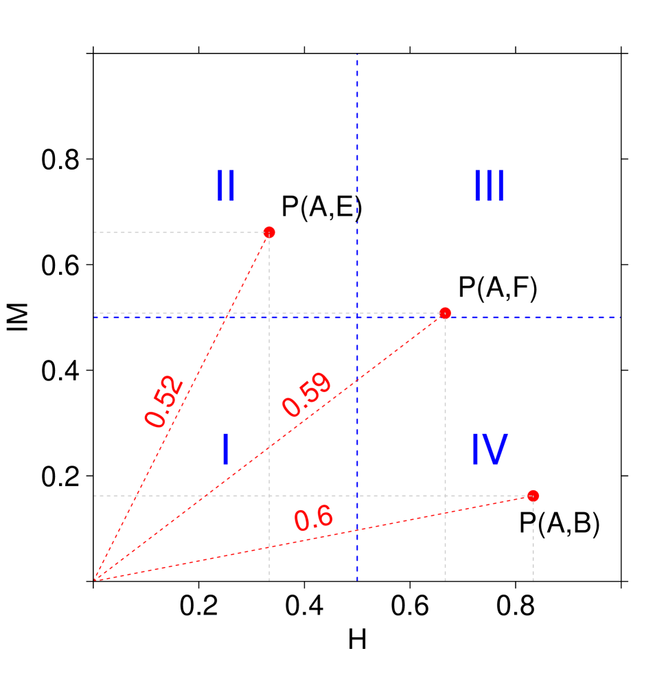
(a)	(b)

Figure 1: An example of HIM distance. (a) Network A (top) and Network B (bottom); (b) Representation of the HIM distance in the Ipsen-Mikhailov and Hamming distance space between networks A versus B, C and D, where C is the fully connected network and D is the empty one.

Finally, the HIM distance is defined as the product metric of the normalized Hamming distance H and the normalized Ipsen-Mikhailov IM distance, normalized by the factor $\sqrt{2}$ to set its upper bound to 1:

$$\textrm{HIM}(N_{1},N_{2})=\frac{1}{\sqrt{2}}\sqrt{\text{H}(N_{1},N_{2})^{2}+\text{IM}(N_{1},N_{2})^{2}}$$

We can represent the HIM distance in the $[0,1]\times[0,1]$ Hamming/Ipsen-Mikhailov space, where a point $P(x,y)$ represents the distance between two networks $N_{1}$ and $N_{2}$ whose coordinates are $x=\text{H}(N_{1},N_{2})$ and $y=\text{IM}(N_{1},N_{2})$ and the norm of $P$ is $\sqrt{2}$ times the HIM distance $\text{HIM}(N_{1},N_{2})$. The same holds for weighted networks, provided that the weights range in $[0;1]$. In Fig. 1 we provide an example of this representation of the HIM distance between networks of four nodes. Roughly splitting the Hamming/Ipsen-Mikhailov space into four main zones I,II,III,IV as in Figure 1, we can say that two networks whose distances correspond to a point in zone I are quite close both in terms of matching links and of structure, while those falling in the zone III are very different with respect to both characteristics. Networks corresponding to a point in zone II have many common links, but their structure is rather different, while a point in zone IV indicates two networks with few common links, but with similar structure. Full mathematical details about the HIM distance and its two components H and IM are available in (Jurman et al., 2012).

2.2 Stability indicators

1. Given a dataset $D$ with $s$ samples and $p$ features, reconstruct (with a chosen algorithm ALG) the network $N_{D}$ on the whole dataset $D$; denote the $p$ nodes of $N_{D}$ by $x_{1}^{D},\ldots,x_{p}^{D}$ and its edges’ weight by $a_{hk}^{D}$, for $k,h=1,\ldots,p$. 2. Choose two integers $n,r$ with $n<s$ and $r\leq\binom{s}{n}$, and build a set $\mathcal{D}_{(n,r)}=\{D_{1},\ldots D_{r}\}$ where $D_{i}$ is a dataset built choosing $n$ samples from $D$. 3. Reconstruct, by using the same algorithm ALG, the corresponding networks $N_{D_{i}}$ on the subsampled data. 4. Compute the following indicators: • $I_{1}(n,r)=\{\textrm{HIM}(N_{D},N_{D_{i}})\colon i=1,\ldots,r\}$ • $I_{2}(n,r)=\{\textrm{HIM}(N_{D_{i}},N_{D_{j}})\colon i,j=1,\ldots r,i\not=j\}$ • $I_{3}(n,r)=\{a_{hk}^{D_{i}}\}$ for $i=1,\ldots,r$ and $k,h=1,\ldots,p$ • $I_{4}(n,r)=\{\partial(x_{h}^{D_{i}})\}$ for $i=1,\ldots,r$ and $h=1,\ldots,p$ and $\partial$ the degree function. 5. For each set of values $I_{i}$ compute the mean, the range (defined as the difference between maximum and minumum value) and the 95% studentized bootstrap confidence intervals (Davison and Hinkley, 1997) as implemented in the R package boot (Canty and Ripley, 2012). 6. Comparative analysis of the statistics of the four indicators $I_{1},\ldots I_{4}$ will describe the level of confidence (stability) in the network $N_{D}$, in its links and in its nodes.

Figure 2: Definition of the four stability indicators $I_{1},\ldots,I_{4}$.

We introduce now the four stability indicators, for a given subset of the original data and a given number of replicates, producing a set of corresponding inferred networks. The first two indicators concern the stability of the entire network, measuring the mutual distances of the networks inferred from the different replicates and their distances to the network constructed on the whole dataset. The other two indicators concern instead the stability (and thus the reliability) of the single nodes and links, in terms of mutual variability of their respective degree and weight. In Fig. 2 we detail the mathematical formulation of the four indicators: the smaller the indicators’ values, the stabler the indicators’ targets. In particular, for all experiments on both synthetic and biological datasets we used $n=s-1$, $r=1$ [leave-one-out stability, LOO for short], and $20$ different instances of $k$-fold cross validation (discarding the test portion) for $k=2,4,10$ (denoted by $k2$, $k4$ and $k10$ in what follows), and thus $n=\lfloor\frac{s(k-1)}{k}\rfloor$ and $r=20k$.

3 RESULTS

3.1 FDR effect on correlation networks

As a first experiment, we want to assess the different level of stability in a correlation network inferred by a set of synthetic high-throughput signals when the inference (absolute value of Pearson correlation) is computed with or without False Discovery Rate control (see for instance (Jiao et al., 2011)). As the correlation measure, we use the classical (absolute) Pearson correlation of the WGCNA (Horvath, 2011) and the novel correlation measure called Maximal Information Coefficient (MIC), component of the Maximal Information-based Nonparametric Exploration (MINE) statistics (Reshef et al., 2011; Speed, 2011; Nature Biotechnology, 2012). For a set of values $n<m$ and an adequate number of resampling $r=\min\{20,\binom{m}{n}\}$, compute the indicators $I_{j}(n,r)$ for $j=1,\ldots,4$ for all the used algorithms.

1. Let $D$ a dataset with $m$ samples described by $q$ features, and let $C(h,k)=|\textrm{cor}(x_{h},x_{k})|$ where $x_{j}$ is the $j$-th feature of $D$ across the $m$ samples and cor is a correlation measure. 2. Build the standard correlation network $N_{D}$ using the rule $a_{hk}=C(h,k)$ 3. Build the FDR controlled (at $p$-value $\wp=10^{-z}$) correlation network $M^{\wp}_{D}$ using the rule $$a_{hk}=\begin{cases}C(h,k)&\textrm{if $|F^{z}_{D}(h,k)|\leq 1$}\\ 0&\textrm{otherwise, }\end{cases}$$ where the set $F_{z}$ is defined as follows $$F^{z}_{D}=\{\textrm{cor}(\sigma_{i}(x_{h}),\tau_{i}(x_{k}))\geq C(h,k)\colon\sigma_{i},\tau_{i}\in S_{m},i=1,\ldots,\max\{10^{z},m!\}\}$$ (3)

Figure 3: Construction of a FDR-corrected correlation network.

3.1.1 Data generation

As a synthetic benchmark for evaluating differences between Pearson and MIC correlation measures, and to assess the impact of the FDR filter on the construction of a correlation network, we built a dataset $S$ consisting of 100 measurements (samples) of 20 variables (features) $f_{i}$, from which we constructed the corresponding correlation networks on $20$ nodes. The dataset $S$ was generated starting from its correlation matrix $M_{S}$, which was randomly generated with the following three constraints:

$$\textrm{Corr}(f_{i},f_{j})\approx\begin{cases}0.9&\textrm{for $1\leq i\not=j\leq 5$}\\ 0.7&\textrm{for $6\leq i\not=j\leq 10$}\\ 0.4&\textrm{for $11\leq i\not=j\leq 16$}\ ,\end{cases}$$

for Corr the Pearson correlation. The correlation matrix $M_{S}$ is plotted in Fig. 4: clearly, the correlation values in the three groups defined by the above constraints represent true relations between the variables, while all other smaller correlation values are due to the underlying random generation model for $M_{S}$.

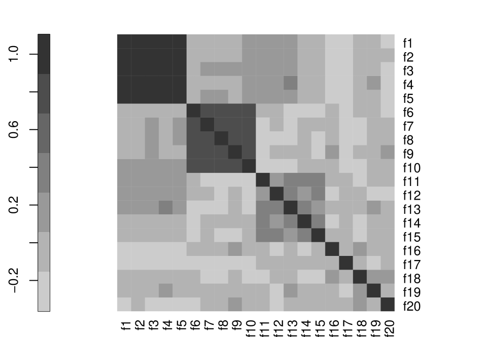
Figure 4: The correlation matrix $M_{S}$ used to generate the synthetic dataset $S$

3.1.2 Results

Starting from the dataset $S$ we built five correlation networks, using MIC, absolute Pearson correlation without FDR correction (WGCNA) and absolute Pearson correlation with FDR correction, with $p$-values $\wp=10^{-2},5\cdot 10^{-3},10^{-4}$. The plots of the graphs for three of the networks are displayed in Fig. 5. As expected, while the WGCNA networks with highest FDR correction $\wp=10^{-4}$ is discarding all links as not significant apart from the edges connecting the two disjoint sets of nodes $\{f_{i}\colon 1\leq i\leq 5\}$ and $\{f_{i}\colon 6\leq i\leq 11\}$ (the strongest correlations in the matrix $M_{S}$), WGNCA and MIC generates two fully connected networks with a majority of weak links.

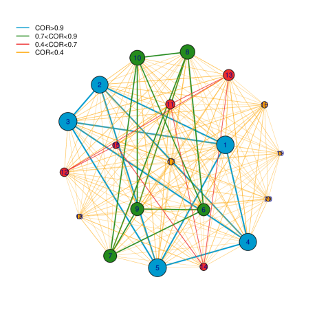
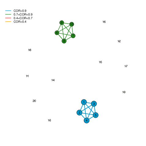
(a) WGCNA	(b) WGCNA FDR 1e-4
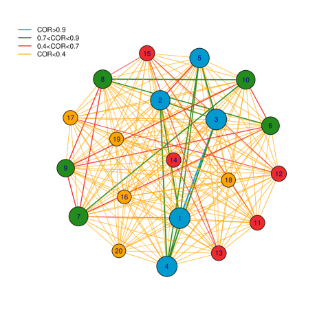
(c) MIC

Figure 5: Correlation networks inferred by the dataset $S$ using (a) absolute Pearson, (b) absolute Pearson with FDR correction at $p$-value $10^{-4}$ and (c) MIC. Node label $i$ corresponds to feature $f_{i}$, node size is proportional to node degree and link colors identify different classes of link weights.

Then we computed the four indicators $I_{1},\ldots I_{4}$ for all the five networks described above, in the setup described in Sec. 2.2.

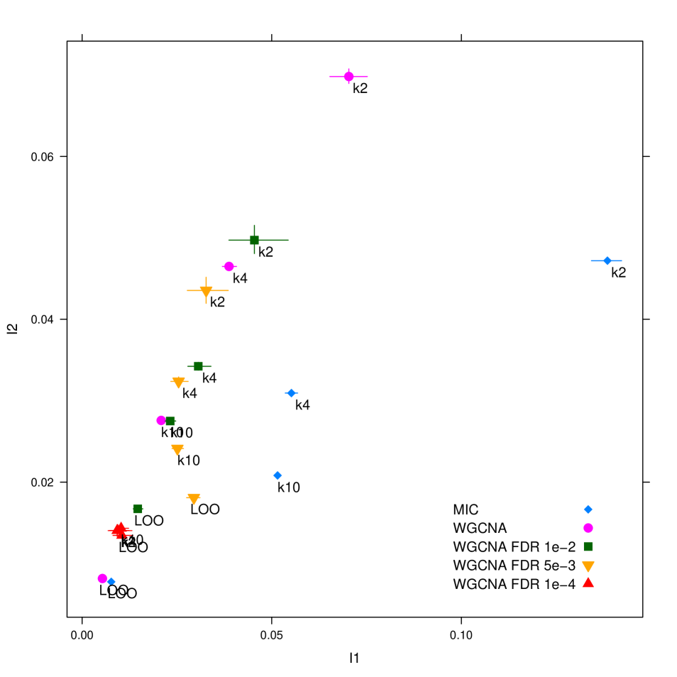
Figure 6: $I_{1}$ and $I_{2}$ stability indicators (mean and confidence intervals) for different instances of the WGCNA and MIC networks on the dataset $S$ and for different values of data subsampling.

Main statistics for all the indicators $I_{1}$ and $I_{2}$ are reported in Tab. 1 and displayed in Fig. 6.

Table 1: Statistics (mean, bootstrap confidence intervals and range) of the stability indicators $I_{1}$ and $I_{2}$ for different instances of the WGCNA and MIC networks on the dataset $S$ and for different values of data subsampling.

ALG	k	I	mean	CI lower	CI upper	min	max
MIC	k10	$I_{1}$	0.052	0.051	0.052	0.041	0.067
MIC	k10	$I_{2}$	0.021	0.021	0.021	0.014	0.036
MIC	k2	$I_{1}$	0.139	0.134	0.142	0.112	0.158
MIC	k2	$I_{2}$	0.047	0.047	0.048	0.035	0.067
MIC	k4	$I_{1}$	0.055	0.054	0.057	0.040	0.071
MIC	k4	$I_{2}$	0.031	0.031	0.031	0.022	0.045
MIC	LOO	$I_{1}$	0.008	0.007	0.008	0.004	0.011
MIC	LOO	$I_{2}$	0.008	0.008	0.008	0.003	0.014
WGCNA	k10	$I_{1}$	0.021	0.020	0.022	0.011	0.040
WGCNA	k10	$I_{2}$	0.028	0.028	0.028	0.012	0.064
WGCNA	k2	$I_{1}$	0.070	0.065	0.076	0.037	0.108
WGCNA	k2	$I_{2}$	0.070	0.069	0.071	0.042	0.117
WGCNA	k4	$I_{1}$	0.039	0.037	0.041	0.020	0.062
WGCNA	k4	$I_{2}$	0.046	0.046	0.047	0.025	0.088
WGCNA	LOO	$I_{1}$	0.005	0.005	0.006	0.001	0.015
WGCNA	LOO	$I_{2}$	0.008	0.008	0.008	0.002	0.023
WGCNA FDR 1e-2	k10	$I_{1}$	0.023	0.022	0.025	0.007	0.074
WGCNA FDR 1e-2	k10	$I_{2}$	0.028	0.027	0.028	0.002	0.102
WGCNA FDR 1e-2	k2	$I_{1}$	0.045	0.039	0.054	0.014	0.107
WGCNA FDR 1e-2	k2	$I_{2}$	0.050	0.048	0.051	0.006	0.152
WGCNA FDR 1e-2	k4	$I_{1}$	0.031	0.028	0.034	0.010	0.069
WGCNA FDR 1e-2	k4	$I_{2}$	0.034	0.034	0.035	0.006	0.096
WGCNA FDR 1e-2	LOO	$I_{1}$	0.015	0.013	0.016	0.005	0.035
WGCNA FDR 1e-2	LOO	$I_{2}$	0.017	0.017	0.017	0.001	0.047
WGCNA FDR 5e-3	k10	$I_{1}$	0.025	0.024	0.027	0.004	0.054
WGCNA FDR 5e-3	k10	$I_{2}$	0.024	0.024	0.024	0.001	0.083
WGCNA FDR 5e-3	k2	$I_{1}$	0.033	0.028	0.038	0.008	0.070
WGCNA FDR 5e-3	k2	$I_{2}$	0.044	0.042	0.045	0.002	0.121
WGCNA FDR 5e-3	k4	$I_{1}$	0.025	0.023	0.028	0.006	0.056
WGCNA FDR 5e-3	k4	$I_{2}$	0.032	0.032	0.033	0.004	0.099
WGCNA FDR 5e-3	LOO	$I_{1}$	0.029	0.028	0.031	0.003	0.048
WGCNA FDR 5e-3	LOO	$I_{2}$	0.018	0.018	0.018	0.000	0.054
WGCNA FDR 1e-4	k10	$I_{1}$	0.010	0.009	0.012	0.000	0.053
WGCNA FDR 1e-4	k10	$I_{2}$	0.014	0.014	0.015	0.000	0.055
WGCNA FDR 1e-4	k2	$I_{1}$	0.009	0.007	0.013	0.001	0.031
WGCNA FDR 1e-4	k2	$I_{2}$	0.014	0.013	0.015	0.001	0.040
WGCNA FDR 1e-4	k4	$I_{1}$	0.009	0.007	0.012	0.001	0.049
WGCNA FDR 1e-4	k4	$I_{2}$	0.014	0.014	0.014	0.001	0.054
WGCNA FDR 1e-4	LOO	$I_{1}$	0.010	0.008	0.013	0.000	0.044
WGCNA FDR 1e-4	LOO	$I_{2}$	0.013	0.013	0.014	0.000	0.045

As expected, the ratio of the discarded data has a strong impact on both the indicators $I_{1}$ and $I_{2}$: in the leave-one-out case the indicators’ values are close to zero regardless of the algorithm, while in the $k$-fold cross-validation case the stability is worsening for decreasing values of $k$, in terms of both mean and confidence intervals. This means that the networks inferred from a subset of data have larger distance both mutually and from the network reconstructed from the whole datasets, but also that these distances have larger variability. From the point of view of the different algorithms involved, the stricter the $p$-value in the FDR controlled WGCNA networks, the stabler the networks, with non controlled WGCNA and MINE as the worst performer in terms of stability. This is due to the fact that they are taking into account all possible correlation values, while most of the smaller values do not represent existing relations between variables, but they are rather a noise effect. As a first result then we showed that the use of a FDR control procedure for correlation help stabilizing the inference procedure, improving the performance of a method already acknowledged as effective (Allen et al., 2012).

We move now on to discuss the stablest links and nodes in the three cases WGCNA, WGCNA FDR 1e-4 and MIC: in particular, in Tab. 2 and 3 we show the top-ranked links and nodes ordered for decreasing range over mean of their weights across all resampling $k4$.

Table 2: Top ranked links, ordered by weight range over weight mean across all 20 resampling of $k4$ $4$-fold cross validation, for the three algorithms WGCNA, WGCNAFDR1e-4 and MIC

WGCNA		WGCNA FDR 1e-4		MIC
$f_{i}-f_{j}$	Range/Mean	$f_{i}-f_{j}$	Range/Mean	$f_{i}-f_{j}$	Range/Mean
1 - 3	0.03	1 - 3	0.03	3 - 4	0.20
2 - 3	0.04	3 - 4	0.04	2 - 3	0.20
1 - 2	0.04	2 - 3	0.04	1 - 3	0.21
1 - 4	0.04	1 - 4	0.05	3 - 5	0.22
3 - 4	0.04	3 - 5	0.05	1 - 2	0.23
2 - 4	0.04	1 - 2	0.05	1 - 5	0.25
4 - 5	0.04	2 - 4	0.05	1 - 4	0.26
2 - 5	0.05	2 - 5	0.06	4 - 5	0.27
1 - 5	0.05	4 - 5	0.06	7 - 10	0.28
3 - 5	0.05	1 - 5	0.06	7 - 8	0.29
6 - 8	0.08	6 - 8	0.08	6 - 8	0.29
8 - 10	0.10	7 - 8	0.09	6 - 10	0.30
7 - 8	0.11	8 - 10	0.10	1 - 20	0.31
7 - 9	0.11	8 - 9	0.11	2 - 4	0.31
8 - 9	0.11	6 - 7	0.11	8 - 10	0.31
9 - 10	0.11	7 - 10	0.12	2 - 5	0.32
6 - 7	0.11	7 - 9	0.12	9 - 10	0.32
7 - 10	0.12	9 - 10	0.13	7 - 20	0.33
6 - 10	0.13	6 - 9	0.13	14 - 16	0.33
6 - 9	0.14	6 - 10	0.15	5 - 17	0.35
11 - 13	0.33			6 - 7	0.35
14 - 15	0.41			11 - 17	0.36
13 - 14	0.46			6 - 9	0.36
12 - 13	0.58			1 - 10	0.37
12 - 15	0.60			10 - 11	0.37
11 - 14	0.62			10 - 20	0.37
13 - 15	0.71			4 - 17	0.37
11 - 15	0.78			2 - 8	0.37
14 - 18	0.78			4 - 10	0.37
3 - 11	0.83			6 - 13	0.37
5 - 11	0.83			2 - 14	0.37
1 - 11	0.84			9 - 11	0.38
4 - 11	0.85			15 - 16	0.38
3 - 10	0.87			15 - 17	0.38
5 - 16	0.89			7 - 13	0.39
8 - 17	0.89			9 - 18	0.39
2 - 11	0.91			12 - 19	0.39
8 - 12	0.91			6 - 18	0.39
4 - 13	0.91			8 - 9	0.39
1 - 13	0.93			4 - 18	0.39
3 - 13	0.93			16 - 17	0.39
8 - 13	0.94			4 - 19	0.39
9 - 17	0.94			16 - 19	0.39
1 - 16	0.95			7 - 19	0.40
1 - 10	0.95			5 - 8	0.40
14 - 16	0.97			14 - 15	0.40
5 - 10	0.97			13 - 15	0.40
11 - 12	0.98			4 - 11	0.40
12 - 16	0.98			7 - 9	0.41
2 - 13	0.99			13 - 19	0.41

The results collected in the tables are consistent with the structure of the starting correlation matrix $M_{S}$ and the behaviour of the inference algorithms. For the WGCNA case, the top $20$ stablest links are those of the two fully connected subgroups $F_{1,5}=\{f_{i}\colon 1\leq i\leq 5\}$ and $F_{6,10}\{f_{i}\colon 6\leq i\leq 10\}$ with largest Pearson correlation values in $M_{S}$. The same applies to WGCNA FDR 1e-4 (and with approximately the same values of weight range over weight mean as for WGCNA), for which these 20 links are the only existing (see Fig. 5). Among the following ranked links in WGCNA, those belonging to the $F_{11,15}=\{f_{i}\colon 11\leq i\leq 15\}$ group (whose correlation of about 0.3 was imposed as a constraint for $M_{S}$) are emerging, with a couple of exceptions, but with larger instability values (0.33-0.78 vs. 0.03-0.14). The remaining links are the unstablest, displaying Range/Mean values always larger than 0.83: they are the randomly correlated links of $M_{S}$. It is interesting to note that the MIC network, due to the nature of the MIC statistics aimed at detecting relations between variables other than linear, displays similar but not identical results: the values of Range/Mean are confined in a narrower interval, and, although many links belonging to the $F_{1,5}$ and $F_{6,10}$ groups are highly ranked, some of them can also be found in much lower positions of the standing.

Similar considerations hold for the ranking of the stablest nodes: for WGCNA, the top ranking nodes are the $F_{1,5}$ and the $F_{6,10}$ (with similar Range/Mean values), with those in $F_{11,15}$ come next, leaving the remaining five as the most unstable, with higher Range/Mean values. These five nodes, on the contrary, are the stablest for WGCNA FDR 1e-4: in fact, they are not wired to any other node in any of the resampling, so their Range/Mean values are void. The nodes $F_{1,5}\cup F_{6,10}$ then follow in the ranking with small associated values, and the nodes $F_{11,15}$ close the standing with definitely higher values. In fact, although the nodes $F_{11,15}$ have degree zero in the WGCNA FDR 1e-4 inferred from the whole $S$, some links involving them exist in some of the resampling on the subset of data. To conclude with, in the MIC case again the ranking values span a much narrower range than the other two cases, and the obtained dwranking has most of the nodes in $F_{1,5}$ in top positions, while for the other nodes the relation with the structure of $M_{S}$ is very weak.

Finally, the analogous tables for other ratios of the data subsampling schema (LOO, $k2$ and $k10$) are almost identical.

Table 3: Top ranked nodes, ordered by degree range over degree mean across all 20 resampling of $k4$ $4$-fold cross validation, for the three algorithms WGCNA, WGCNA FDR 1e-4 and MIC. (*) indicates that Ratio and Mean are both zero.

WGCNA		WGCNA FDR 1e-4		MIC
$f_{i}$	Range/Mean	$f_{i}$	Range/Mean	$f_{i}$	Range/Mean
4	0.17	16	0*	3	0.08
10	0.18	17	0*	19	0.08
3	0.20	18	0*	1	0.08
1	0.21	19	0*	4	0.09
9	0.23	20	0*	8	0.09
2	0.23	3	0.03	10	0.09
5	0.24	1	0.04	5	0.10
7	0.24	2	0.04	2	0.10
6	0.24	5	0.05	17	0.10
8	0.25	7	0.07	20	0.10
11	0.40	8	0.07	15	0.11
13	0.40	6	0.09	9	0.11
15	0.43	9	0.09	13	0.11
12	0.45	10	0.09	11	0.11
14	0.48	4	0.13	16	0.11
18	0.55	15	4.42	12	0.11
16	0.60	14	7.05	7	0.11
17	0.68	12	22.82	6	0.12
20	0.70	13	26.05	14	0.13
19	1.15	11	41.83	18	0.13

3.2 miRNA network on a Hepatocellular Carcinoma dataset

Investigating the relations connecting human microRNA (miRNA) and how they evolve in cancer has been recently a key topic for researcher in biology (Volinia et al., 2010; Bandyopadhyay et al., 2010), with hepatocellular carcinoma (HCC) as a notable example (Law and Wong, 2011; Gu et al., 2012). In the following example, we use the stability indicators $I_{1},\ldots,I_{4}$ on a recent miRNA microarray dataset with two phenotypes to highlight differences in the corresponding inferred networks. As reconstruction algorithm we use the Context Likelihood of Relatedness (CLR) approach (Faith et al., 2007), belonging to the relevance networks class of algorithms and generating undirected weighted graphs with weights bounded between zero and one. In particular, interactions are scored by using the mutual information between the corresponding gene expression levels coupled with an adaptive background correction step. Although suboptimal if the number of variables is much larger than the number of variables, it was observed that CLR performes well in terms of prediction accuracy and some CLR predictions in literature were later experimentally validated (Ambroise et al., 2012).

3.2.1 Data description

We start out from the Hepatocellular Carcinoma dataset introduced in the paper (Budhu et al., 2008) and later used in (Ji et al., 2009), publicly available at the Gene Expression Omnibus (GEO, http://www.ncbi.nlm.nih.gov/geo/) at the accession number GSE6857. The dataset collects 482 tissue samples from 241 patients affected by hepatocellular carcinoma (HCC). For each patients, a sample from cancerous hepatic tissue and a sample from surrounding non-cancerous hepatic tissue are available, hybridized on the Ohio State University CCC MicroRNA Microarray Version 2.0 platform consisting of 11520 probes collecting expressions of 250 non-redundant human and 200 mouse microRNA (miRNA). After a preprocessing phase including imputation of missing values as in (Troyanskaya et al., 2001) and discarding probes corresponding to non-human (mouse and controls) miRNA, we end up with the dataset $\mathcal{HCC}$ of 240+240 paired samples described by 210 human miRNA, with the cohort consisting of 210 male and 30 female patients. We thus parted the whole dataset $\mathcal{HCC}$ into four subsets combining the sex and disease status phenotypes, collecting respectively the cancer tissue for the male patients (MT), the cancer tissue for the female patients (FT) and the corresponding two datasets including the non cancer tissues (MnT, FnT).

3.2.2 Results

Using the CLR algorithm we first generated the four networks inferred from the whole sets of data and corresponding to the combinations of the two binary phenotypes: a portrait of the resulting graphs is depicted in Fig. 8, discarding links whose weight is smaller than 0.1. As a first observation, the four networks have a different structure, for instance the tumoral tissues graphs being more connected than the controls and the female graphs more than the corresponding male ones (see for instance the density values in Fig. 8). In particular, their mutual HIM distances are reported in Tab. 7, together with the corresponding two-dimensional scaling plot, showing that the networks corresponding to the female patients (and, in particular, the one inferred from cancer tissue) are notably different from those arising from the subset of data for the male patients.

MnT FT FnT 0.0412 0.0858 0.0235 MT 0.1265 0.0618 MnT 0.0684 FT

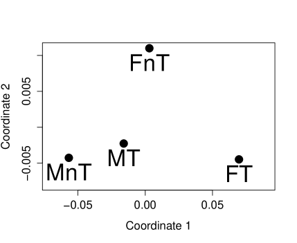
Figure 7: Mutual HIM distances for the four CLR inferred networks MT, MnT, FT, FnT reconstructed from the whole corresponding subsets and corresponding 2D multidimensional scaling plot.

We then computed the stability indicators $I_{1}$ and $I_{2}$ in the setup described in Sec. 2.2, and the corresponding statistics are collected and displayed in Tab. 4 and Fig. 9.

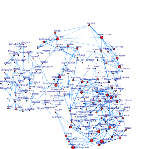
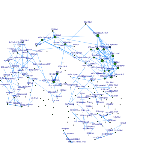
(a) MT, $d=0.0153$	(b) MnT, $d=0.0092$
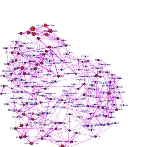
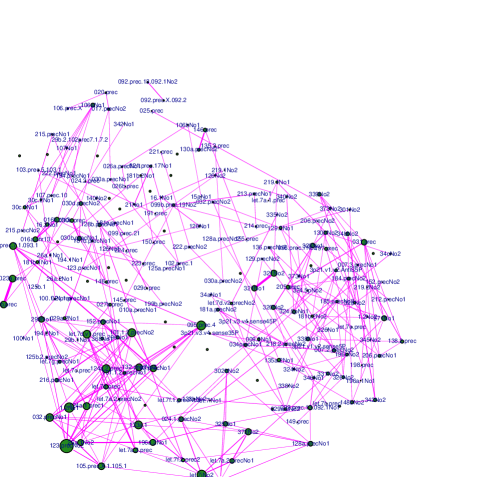
(c) FT, $d=0.0206$	(d) FnT, $d=0.0121$

Figure 8: CLR networks (and corresponding density values) inferred from the 4 subsets (a) Male Tumoral (MT) (b) Male not Tumoral (MnT) (c) Female Tumoral (FT) and (d) Female non Tumoral (FnT) of the datasets $\mathcal{HCC}$. Links are thresholded at weight 0.1, node position is fixed across the four networks, node dimension is proportional to the degree and edge width is proportional to link weight.

It is immediately evident the different sample size impact on the network stability: the networks corresponding to male patients have smaller values for $I_{1}$ and $I_{2}$ (and thus they are much stabler) than the corresponding female counterparts, and this effect is even stronger than the one due to the ratio of the chosen subsets of data: the leave-one-out stability for FT and FnT is worse than k10 and k4 stability for MT and MnT. On the other hand, while control and cancer networks display similar level of stability in the male networks at all levels of subsampling ratio, in the female group the network associated to the controls is much stabler than the matching control networks, and this is evident when the size of the subset used for inference gets smaller, in particular for $k=2$.

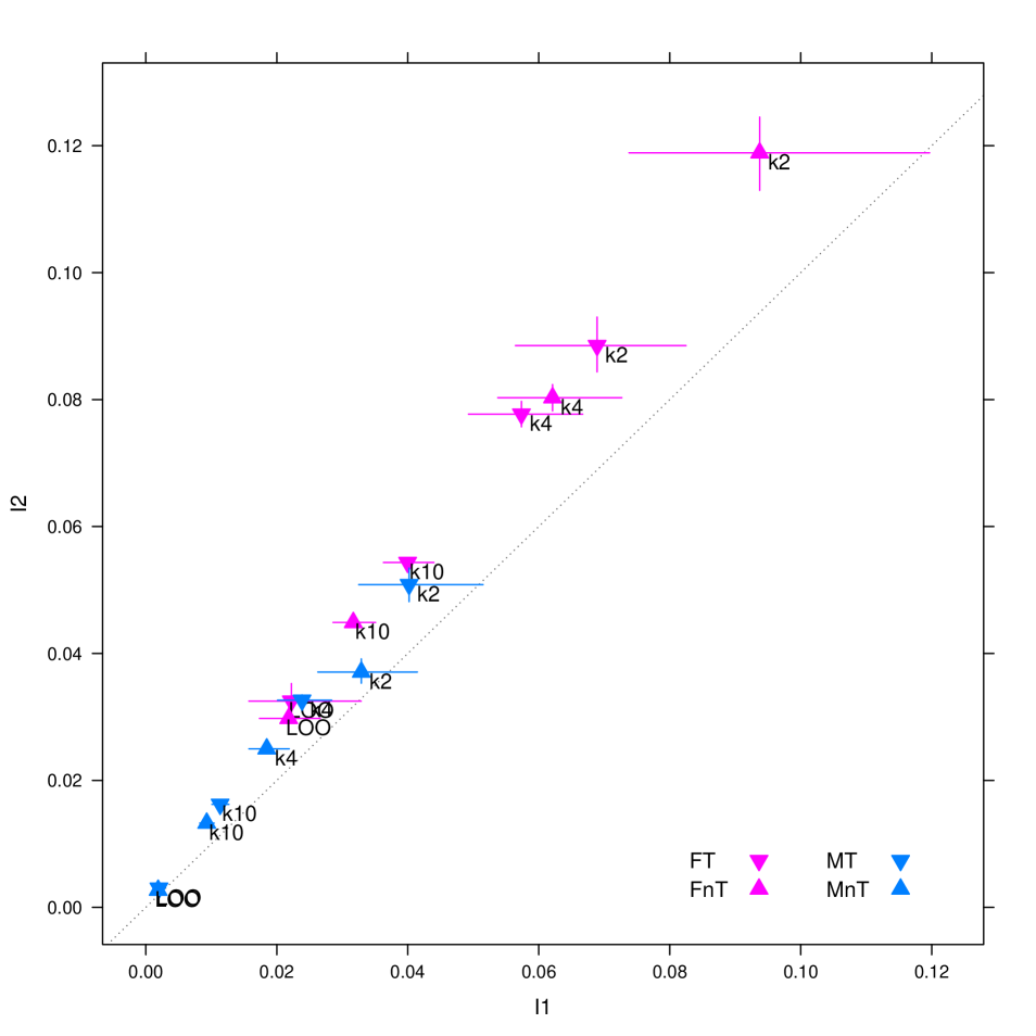
Figure 9: $I_{1}$ and $I_{2}$ stability indicators (mean and confidence intervals) of CLR inferred networks for different values of data subsampling on the four subgroups Male Tumoral (MT), Male not Tumoral (MnT), Female Tumoral (FT) and Female non Tumoral (FnT) of the datasets $\mathcal{HCC}$.

Table 4: Statistics (mean, bootstrap confidence intervals and range) of the stability indicators $I_{1}$ and $I_{2}$ for the CLR inferred networks on the datasets MT, MnT, FT, FnT, for different values of data subsampling.

PROBL	k	I	mean	lower	upper	min	max
FT	k10	$I_{1}$	0.040	0.037	0.044	0.002	0.177
FT	k10	$I_{2}$	0.054	0.054	0.055	0.000	0.256
FT	k2	$I_{1}$	0.069	0.056	0.082	0.006	0.154
FT	k2	$I_{2}$	0.089	0.084	0.093	0.005	0.250
FT	k4	$I_{1}$	0.057	0.049	0.066	0.004	0.190
FT	k4	$I_{2}$	0.078	0.076	0.080	0.003	0.305
FT	LOO	$I_{1}$	0.022	0.016	0.032	0.002	0.093
FT	LOO	$I_{2}$	0.032	0.030	0.035	0.001	0.143
FnT	k10	$I_{1}$	0.032	0.029	0.035	0.002	0.093
FnT	k10	$I_{2}$	0.045	0.044	0.045	0.000	0.179
FnT	k2	$I_{1}$	0.094	0.071	0.117	0.006	0.257
FnT	k2	$I_{2}$	0.119	0.113	0.124	0.006	0.391
FnT	k4	$I_{1}$	0.062	0.054	0.072	0.005	0.203
FnT	k4	$I_{2}$	0.080	0.078	0.082	0.003	0.307
FnT	LOO	$I_{1}$	0.022	0.017	0.027	0.003	0.048
FnT	LOO	$I_{2}$	0.030	0.028	0.032	0.001	0.094
MT	k10	$I_{1}$	0.011	0.010	0.013	0.001	0.048
MT	k10	$I_{2}$	0.016	0.016	0.016	0.001	0.092
MT	k2	$I_{1}$	0.040	0.033	0.051	0.003	0.146
MT	k2	$I_{2}$	0.051	0.048	0.054	0.003	0.218
MT	k4	$I_{1}$	0.024	0.020	0.029	0.002	0.099
MT	k4	$I_{2}$	0.033	0.032	0.033	0.001	0.148
MT	LOO	$I_{1}$	0.002	0.002	0.002	0.000	0.018
MT	LOO	$I_{2}$	0.003	0.003	0.003	0.000	0.030
MnT	k10	$I_{1}$	0.009	0.008	0.010	0.001	0.034
MnT	k10	$I_{2}$	0.013	0.013	0.013	0.001	0.061
MnT	k2	$I_{1}$	0.033	0.026	0.041	0.003	0.104
MnT	k2	$I_{2}$	0.037	0.035	0.039	0.002	0.158
MnT	k4	$I_{1}$	0.018	0.015	0.022	0.001	0.067
MnT	k4	$I_{2}$	0.025	0.024	0.026	0.001	0.102
MnT	LOO	$I_{1}$	0.002	0.002	0.002	0.000	0.009
MnT	LOO	$I_{2}$	0.003	0.003	0.003	0.000	0.016

Finally, to show how to use indicators $I_{3}$ and $I_{4}$ to extract information about stability of some interesting links, we first rank all links according to their weight Range/Mean value for all the four cases MT, MnT, FT, FnT, and then we point out six links worth a comment, listed in Tab. 5. The link (a) is top ranking in all four cases as expected, since hsa-mir_321No1 and hsa-mir_321No2 denote essentially the same miRNA (identical or with very similar sequences, (Ambros et al., 2003). The same applies to the links (b) and (c), but in these cases the stability of these two links in the FnT network is not as good as in the other three cases, probably due to the presence of noise in the data. The link (d) is interesting because of the difference of its stability between the male and the female networks, indicating a link probably associated to sex rather than HCC. The behaviour of link (e) is even more singular: it is one of the stablest links for the FT network, while is not even picked up as a link by CLR in the FnT network. Finally, link (f) is a very well known connection in literature, strongly associated to cancer (Volinia et al., 2010; Braun et al., 2008; Georges et al., 2008) as confirmed by its high stability in the MT and FT networks only.

Table 5: Position in the weight Range/Mean ranking in the four cases MT, MnT, FT, FnT for six miRNA-miRNA links.

id	hsa-mir_idx1	hsa-mir_idx2	MT	MnT	FT	FnT
(a)	321No1	321No2	1	1	9	2
(b)	016b.chr3	16.2No1 3	12	15	309
(c)	021.prec.17No1	21No1	27	5	2	921
(d)	219.1No1	321No2	2	6	1903	314
(e)	326No1	342No2	132	1017	3	-
(f)	192.2.3No1	215.precNo1	4	300	4	3340

4 CONCLUSIONS

We introduced a suite of four stability indicators for assessing the variability of network reconstruction algorithm as functions of a data subsampling procedure. The aim here is to provide the researchers with an effective tool to compare either the inference algorithms or the investigated dataset. Two indicators are based on a measure of a normalized distance between networks and they are global, giving a confidence measure on the whole inferred dataset, while the other two are local, associating a reliability score to the network nodes and detected links. They are of particular interest when no gold standard is known for the studied task, so they can work as a substitute for the algorithm accuracy. We demonstrated their consistency on a synthetic dataset, and we showed their use on a high-throughput microarray experiment, with two widely known inference methods such as WGCNA and CLR.

DISCLOSURE STATEMENT

No competing financial interests exist.

Address correspondence to:

Giuseppe Jurman

Fondazione Bruno Kessler (FBK)

via Sommarive 18 - Povo

I-38123 Trento

Italy

E-mail: jurman@fbk.eu

References

- Allen et al. (2012) Allen, J., Xie, Y., Chen, M., Girard, L., and Xiao, G., 2012. Comparing Statistical Methods for Constructing Large Scale Gene Networks. PLoS ONE 7, e29348.
- Altay and Emmert-Streib (2010) Altay, G. and Emmert-Streib, F., 2010. Revealing differences in gene network inference algorithms on the network level by ensemble methods. Bioinformatics 26, 1738–1744.
- Ambroise et al. (2012) Ambroise, J., Robert, A., Macq, B., and Gala, J.-L., 2012. Transcriptional Network Inference from Functional Similarity and Expression Data: A Global Supervised Approach. Statistical Applications in Genetics and Molecular Biology 11, Article 2.
- Ambros et al. (2003) Ambros, V., Bartel, B., Bartel, D., Burge, C., Carrington, J., Chen, X., Dreyfuss, G., Eddy, S., Griffiths-Jones, S., Marshall, M., Matzke, M., Ruvkun, G., and Tuschl, T., 2003. A uniform system for microRNA annotation. RNA 9, 277–279.
- Atay et al. (2006) Atay, F., Bıyıkoğlu, T., and Jost, J., 2006. Network synchronization: Spectral versus statistical properties. Physica D Nonlinear Phenomena 224, 35–41.
- Bandyopadhyay et al. (2010) Bandyopadhyay, S., Mitra, R., Maulik, U., and Zhang, M., 2010. Development of the human cancer microRNA network. Silence 1, 6.
- Baralla et al. (2009) Baralla, A., Mentzen, W., and de la Fuente, A., 2009. Inferring Gene Networks: Dream or Nightmare? Annals of the New York Academy of Science 1158, 246–256.
- Braun et al. (2008) Braun, C., Zhang, X., Savelyeva, I., Wolff, S., Moll, U., Schepeler, T., Ørntoft, T., Andersen, C., and Dobbelstein, M., 2008. p53-Responsive MicroRNAs 192 and 215 Are Capable of Inducing Cell Cycle Arrest. Cancer Research 68, 10094–10104.
- Budhu et al. (2008) Budhu, A., Jia, H.-L., Forgues, M., Liu, C.-G., Goldstein, D., Lam, A., Zanetti, K. A., Ye, Q.-H., Qin, L.-X., Croce, C. M., Tang, Z.-Y., and Wang, X. W., 2008. Identification of Metastasis-Related MicroRNAs in Hepatocellular Carcinoma. Hepatology 47, 897–907.
- Canty and Ripley (2012) Canty, A. and Ripley, B., 2012. boot: Bootstrap R (S-Plus) Functions. R package version 1.3-5.
- Chung (1997) Chung, F., 1997. Spectral Graph Theory. American Mathematical Society.
- Davison and Hinkley (1997) Davison, A. and Hinkley, D., 1997. Bootstrap Methods and Their Applications. Cambridge University Press.
- De Smet and Marchal (2010) De Smet, R. and Marchal, K., 2010. Advantages and limitations of current network inference methods. Nature Reviews Microbiology 8, 717–729.
- Dougherty (2010) Dougherty, E., 2010. Validation of gene regulatory networks: scientific and inferential. Briefings in Bioinformatics 12, 245–252.
- Faith et al. (2007) Faith, J., Hayete, B., Thaden, J., Mogno, I., Wierzbowski, J., Cottarel, G., Kasif, S., Collins, J., and Gardner, T., 2007. Large-Scale Mapping and Validation of Escherichia coli Transcriptional Regulation from a Compendium of Expression Profiles. PLoS Biology 5, e8.
- Georges et al. (2008) Georges, S., Biery, M., Kim, S., Schelter, J., Guo, J., Chang, A., Jackson, A., Carleton, M., Linsley, P., Cleary, M., and Chau, B., 2008. Coordinated Regulation of Cell Cycle Transcripts by p53-Inducible microRNAs, miR-192 and miR-215. Cancer Research 68, 10105–10112.
- Gillis and Pavlidis (2011) Gillis, J. and Pavlidis, P., 2011. The role of indirect connections in gene networks in predicting function. Bioinformatics 27, 1860–1866.
- Gu et al. (2012) Gu, Z., Zhang, C., and Wang, J., 2012. Gene regulation is governed by a core network in hepatocellular carcinoma. BMC Systems Biology 6, 32.
- He et al. (2009) He, F., Balling, R., and Zeng, A.-P., 2009. Reverse engineering and verification of gene networks: Principles, assumptions, and limitations of present methods and future perspectives. Journal of Biotechnology 144, 190–203.
- Horvath (2011) Horvath, S., 2011. Weighted Network Analysis: Applications in Genomics and Systems Biology. Springer.
- Ipsen and Mikhailov (2002) Ipsen, M. and Mikhailov, A., 2002. Evolutionary reconstruction of networks. Physical Review E 66, 046109.
- Ji et al. (2009) Ji, J., Shi, J., Budhu, A., Yu, Z., Forgues, M., Roessler, S., Ambs, S., Chen, Y., Meltzer, P., Croce, C., Qin, L.-X., Man, K., Lo, C.-M., Lee, J., Ng, I., Fan, J., Tang, Z.-Y., Sun, H.-C., and Wang, X., 2009. MicroRNA Expression, Survival, and Response to Interferon in Liver Cancer. New England Journal of Medicine 361, 1437–1447.
- Jiao et al. (2011) Jiao, Y., Lawler, K., Patel, G., Purushotham, A., Jones, A., Grigoriadis, A., Tutt, A., Ng, T., and Teschendorff, A., 2011. DART: Denoising Algorithm based on Relevance network Topology improves molecular pathway activity inference. BMC Bioinformatics 12, 403.
- Jurman et al. (2011) Jurman, G., Visintainer, R., and Furlanello, C., 2011. An introduction to spectral distances in networks. Frontiers in Artificial Intelligence and Applications 226, 227–234.
- Jurman et al. (2012) Jurman, G., Visintainer, R., Riccadonna, S., Filosi, M., and Furlanello, C., 2012. A glocal distance for network comparison. ArXiv:1201.2931 [math.CO].
- Kamburov et al. (2012) Kamburov, A., Stelzl, U., and Herwig, R., 2012. Intscore: a web tool for confidence scoring of biological interactions. Nucleic Acids Research first published online May 30.
- Krishnan et al. (2007) Krishnan, A., Giuliani, A., and Tomita, M., 2007. Indeterminacy of Reverse Engineering of Gene Regulatory Networks: The Curse of Gene Elasticity. PLoS ONE 2, e562.
- Law and Wong (2011) Law, P. T.-Y. and Wong, N., 2011. Emerging roles of microRNA in the intracellular signaling networks of hepatocellular carcinoma. Journal of Gastroenterology and Hepatology 26, 437–449.
- Logsdon and Mezey (2010) Logsdon, B. and Mezey, J., 2010. Gene Expression Network Reconstruction by Convex Feature Selection when Incorporating Genetic Perturbations. PLoS Computational Biology 6, e1001014.
- Madhamshettiwar et al. (2012) Madhamshettiwar, P., Maetschke, S., Davis, M., Reverter, A., and Ragan, M., 2012. Gene regulatory network inference: evaluation and application to ovarian cancer allows the prioritization of drug targets. Genome Medicine 4, 41.
- Marbach et al. (2010) Marbach, D., Prill, R., Schaffter, T., Mattiussi, C., Floreano, D., and Stolovitzky, G., 2010. Revealing strengths and weaknesses of methods for gene network inference. Proceedings of the National Academy of Science 107, 6286–6291.
- Meyer et al. (2011) Meyer, P., Alexopoulos, L., Bonk, T., Califano, A., Cho, C., de la Fuente, A., de Graaf, D., Hartemink, A., Hoeng, J., Ivanov, N., Koeppl, H., Linding, R., Marbach, D., Norel, R., Peitsch, M., Rice, J., Royyuru, A., Schacherer, F., Sprengel, J., Stolle, K., Vitkup, D., and Stolovitzky, G., 2011. Verification of systems biology research in the age of collaborative competition. Nature Biotechnology 29, 811–815.
- Miller et al. (2012) Miller, M., Feng, X.-J., Li, G., and Rabitz, H., 2012. Identifying Biological Network Structure, Predicting Network Behavior, and Classifying Network State With High Dimensional Model Representation (HDMR). PLoS ONE 7, e37664.
- Nature Biotechnology (2012) Nature Biotechnology, 2012. Finding correlations in big data. Nature Biotechnology 30, 334–335.
- Prill et al. (2010) Prill, R., Marbach, D., Saez-Rodriguez, J., Sorger, P., Alexopoulos, L., Xue, X., Clarke, N., Altan-Bonnet, G., and Stolovitzky, G., 2010. Towards a Rigorous Assessment of Systems Biology Models: The DREAM3 Challenges. PLoS ONE 5, e9202.
- Reshef et al. (2011) Reshef, D., Reshef, Y., Finucane, H., Grossman, S., McVean, G., Turnbaugh, P., Lander, E., Mitzenmacher, M., and Sabeti, P., 2011. Detecting novel associations in large datasets. Science 6062, 1518–1524.
- Speed (2011) Speed, T., 2011. A Correlation for the 21st Century. Science 6062, 1502–1503.
- Spielman (2009) Spielman, D., 2009. Spectral Graph Theory: The Laplacian (Lecture 2). Lecture notes.
- Szederkenyi et al. (2011) Szederkenyi, G., Banga, J., and Alonso, A., 2011. Inference of complex biological networks: distinguishability issues and optimization-based solutions. BMC Systems Biology 5, 177.
- Tönjes and Blasius (2009) Tönjes, R. and Blasius, B., 2009. Perturbation Analysis of Complete Synchronization in Networks of Phase Oscillators. ArXiv:0908.3365.
- Troyanskaya et al. (2001) Troyanskaya, O., Cantor, M., Sherlock, G., Brown, P., Hastie, T., Tibshirani, R., Botstein, D., and Altman, R., 2001. Missing value estimation methods for DNA microarrays. Bioinformatics 17, 520–525.
- Tun et al. (2006) Tun, K., Dhar, P., Palumbo, M., and Giuliani, A., 2006. Metabolic pathways variability and sequence/networks comparisons. BMC Bioinformatics 7, 24.
- Volinia et al. (2010) Volinia, S., Galasso, M., Costinean, S., Tagliavini, L., Gamberoni, G., Drusco, A., Marchesini, J., Mascellani, N., Sana, M., Abu Jarour, R., Desponts, C., Teitell, M., Baffa, R., Aqeilan, R., Iorio, M., Taccioli, C., Garzon, R., Di Leva, G., Fabbri, M., Catozzi, M., Previati, M., Ambs, S., Palumbo, T., Garofalo, M., Veronese, A., Bottoni, A., Gasparini, P., Harris, C., Visone, R., Pekarsky, Y., de la Chapelle, A., Bloomston, M., Dillhoff, M., Rassenti, L., Kipps, T., Huebner, K., Pichiorri, F., Lenze, D., Cairo, S., Buendia, M.-A., Pineau, P., Dejean, A., Zanesi, N., Rossi, S., Calin, G., Liu, C.-G., Palatini, J., Negrini, M., Vecchione, A., Rosenberg, A., and Croce, C., 2010. Reprogramming of miRNA networks in cancer and leukemia. Genome Research 20, 589–599.