Transfer matrix computation of generalised critical polynomials in percolation

Abstract

Percolation thresholds have recently been studied by means of a graph polynomial $P_{B}(p)$, henceforth referred to as the critical polynomial, that may be defined on any periodic lattice. The polynomial depends on a finite subgraph $B$, called the basis, and the way in which the basis is tiled to form the lattice. The unique root of $P_{B}(p)$ in $[0,1]$ either gives the exact percolation threshold for the lattice, or provides an approximation that becomes more accurate with appropriately increasing size of $B$. Initially $P_{B}(p)$ was defined by a contraction-deletion identity, similar to that satisfied by the Tutte polynomial. Here, we give an alternative probabilistic definition of $P_{B}(p)$, which allows for much more efficient computations, by using the transfer matrix, than was previously possible with contraction-deletion.

We present bond percolation polynomials for the $(4,8^{2})$, kagome, and $(3,12^{2})$ lattices for bases of up to respectively 96, 162, and 243 edges, much larger than the previous limit of 36 edges using contraction-deletion. We discuss in detail the role of the symmetries and the embedding of $B$. For the largest bases, we obtain the thresholds $p_{c}(4,8^{2})=0.676\,803\,329\cdots$, $p_{c}(\mathrm{kagome})=0.524\,404\,998\cdots$, $p_{c}(3,12^{2})=0.740\,420\,798\cdots$, comparable to the best simulation results. We also show that the alternative definition of $P_{B}(p)$ can be applied to study site percolation problems.

,

1 Introduction

Since its introduction [1], percolation has provided a wealth of problems for physicists, mathematicians, and computer scientists. One of the most difficult is the analytical determination of critical probabilities. Given an infinite $d-$dimensional lattice $L$, declare each edge of $L$ to be open with probability $p$ and closed with probability $1-p$. Between the regimes of sparse clusters near $p=0$ and the nearly complete filling of space near $p=1$ lies the critical probability (also called the percolation threshold), $p_{c}$, below which all clusters are finite but above which there is an infinite cluster. In site percolation, which we will also consider here, the vertices of the graph are occupied or unoccupied with probability $p$ or $1-p$, and percolation clusters can be defined by declaring an edge open when it connects two occupied vertices.

For $d=1$, percolation is trivial and $p_{c}=1$, but for $d\geq 3$, the problem is completely unsolved. In two dimensions, bond and site probabilities can be found only on a narrow class of lattices formed from self-dual 3-uniform hypergraphs. In these cases the threshold is given as the root in $[0,1]$ of a finite polynomial. Previously, it was shown [2, 3, 4] that the concept of a critical polynomial may be extended to any two-dimensional lattice. The unique root in $[0,1]$ of this polynomial provides the exact $p_{c}$ for lattices in the solvable class, and for unsolved problems, where we call it the generalised critical polynomial, it gives answers that can seemingly be brought arbitrarily close to the exact threshold. Recently, we extended the definition of this polynomial to the full $q$-state Potts model and used it to explore the phase diagram of the kagome lattice [5].

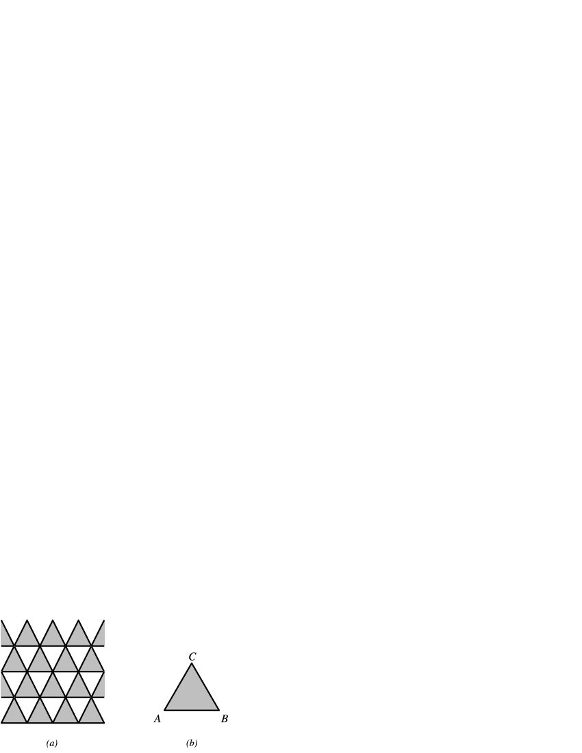
Figure 1: a) A class of self-dual 3-uniform hypergraphs. b) Each shaded triangle may contain arbitrary interactions among its boundary vertices $A$, $B$ and $C$.

2 The generalised critical polynomial

We first consider bond percolation on the self-dual 3-uniform hypergraph depicted in Figure 1a. The particular hypergraph shown is of the simple triangular type, but the argument can be extended to other types of self-dual 3-uniform hypergraphs [6]; one can also treat site percolation problems by reasoning on the covering lattice [7] or by introducting correlations [8]. Interior to the boundary vertices of each shaded triangle (Figure 1b), we may have essentially any network of bonds, correlations, and sites. The critical point of such a system is given by [7, 9]

$$P(A,B,C)=P(\bar{A},\bar{B},\bar{C})\,,$$ (1)

where $P(A,B,C)$ is the probability that all three boundary vertices are connected by an open path in the triangle, and $P(\bar{A},\bar{B},\bar{C})$ is the probability that none are connected. The result of applying this condition is a polynomial in the probability $p$ with degree equal to the number of randomly occupied elements (edges for bond percolation, or vertices for site percolation) within a triangle. Thus, all thresholds that are known exactly are algebraic numbers. We may also consider inhomogeneous percolation in which each edge $i$ is assigned a different probability $p_{i}$ so that (1) provides a critical surface within the space of all $p_{i}$’s.

As already mentioned, a critical polynomial $P_{B}(p)$ can be defined more generally for bond percolation on any two-dimensional lattice [2, 3, 4, 10]. It depends on a finite subgraph $B$, called the basis, and its embedding into the infinite lattice $L$. This $P_{B}(p)$ indeed reproduces the exact percolation threshold (1) for exactly solvable cases, but in general it is only an approximation that however converges very rapidly to the true $p_{c}$ upon appropriately increasing the size of $B$. The definition of $P_{B}(p)$ used in these works proceeds by applying a contraction-deletion principle to the edges in $B$, and by this fact it can be further generalised [5] to a critical polynomial $P_{B}(q,v)$ for the $q$-state Potts model with temperature parameter $v$.

We recall here the contraction-deletion definition of $P_{B}(p)$ by means of a specific example. Consider for $L$ the $(3,12^{2})$ lattice, shown in Figure 2a. Its threshold is not known exactly, but has been the subject of much numerical [11, 12, 13] and analytical [12, 14, 15, 16] work. For the basis $B$ we choose the unit cell shown in Figure 2b with an arbitrary inhomogeneous assignment of probabilities $p_{i}$ to the nine edges. Notice that $B$ is embedded into $L$ in a checkerboard fashion. Any edge of $L$ is a translation of an edge in $B$ and is therefore assigned the corresponding probability $p_{i}$ for some $i=0,1,\ldots,8$.

If we delete the $p_{0}$ edge by setting $p_{0}=0$ in Figure 2b, we obtain the martini lattice (Figure 3a) with some edges coupled in series. Similarly, we can contract the $p_{0}$ edge by setting $p_{0}=1$, and we again find the martini lattice, but with some edges coupled in series and parallel. In both cases, the coupled edges can be replaced by simple edges with appropriate effective percolation probabilities. These considerations lead to the following expression for the critical surface $P_{B}=TT$ of the $(3,12^{2})$ lattice:

$$TT(p_{0},p_{1},\ldots,p_{8}) = p_{0}M(p_{3}[p_{1}+p_{2}-p_{1}p_{2}],p_{4},p_{5},p_{6},p_{7},p_{8})$$ (2)

$$+ (1-p_{0})M(p_{3},p_{2}p_{4},p_{1}p_{5},p_{6},p_{7},p_{8})\,,$$ (3)

where $M$ is the corresponding expression for the martini lattice (Figure 3a) with the inhomogeneous assignment of probabilities to the basis shown in Figure 3b. However, the critical surface of the martini lattice can be found exactly with (1), and inserting this we obtain finally in the homogeneous case the critical polynomial

$$TT(p,p,\ldots,p)=1-3p^{4}-6p^{5}+3p^{6}+15p^{7}-15p^{8}+4p^{9}\,.$$ (4)

The corresponding approximation to the percolation threshold reads $TT(p,p,\ldots,p)=0$, and its unique solution on $[0,1]$ is $p_{c}=0.740\,423\,31\cdots$. Comparing this with the most accurately known numerical value, $p_{c}^{\mathrm{num}}=0.740\,420\,77(2)$ [13], we infer that the prediction provided by the $9^{\mathrm{th}}$-order critical polynomial is close, but not exactly equal to the true $p_{c}$. However, the approximation can be improved by increasing the size of the basis. For example, using the basis of Figure 4, we find a $36^{\mathrm{th}}$-order polynomial, reported in [4], that makes the prediction $p_{c}=0.740\,420\,99\cdots$, which is closer to the numerical value.

Figure 2: a) The $(3,12^{2})$ lattice; b) the assignment of probabilities on the unit cell.

Figure 3: a) The martini lattice; b) the assignment of probabilities on the unit cell.

Figure 4: A $36-$edge basis for the $(3,12^{2})$ lattice. Each edge should be understood to have a different probability, and the shapes on the terminals indicate how this basis is embedded into the lattice.

Critical polynomials $P_{B}(p)$ defined in this way are unique, that is, they are a property only of the basis $B$ and the way in which $B$ is embedded in the infinite lattice $L$. In particular, $P_{B}(p)$ is independent of the order in which edges are contracted-deleted. An important property of $P_{B}(p)$ is that in all exactly solvable cases, the smallest possible basis already provides the exact answer (1), and the same answer invariably factorises from $P_{B}(p)$ upon using a larger basis. On the other hand, for unsolved cases, using appropriate larger bases leads to predictions that improve with the size of $B$, and appear to approach the true $p_{c}$. How close one can get to $p_{c}$ is limited by one’s ability to actually compute the polynomial on large $B$. In [4], a computer program was used to perform the contraction-deletion algorithm on various bases for the Archimedean lattices. However, this algorithm is exponential in the number of edges in $B$, and the upper limit of feasibility was $36$ edges. Nevertheless, the corresponding $P_{B}(p)$ yielded bond percolation thresholds that were generally within $10^{-7}$ of the numerically determined values.

Below, we present an alternative definition of $P_{B}(p)$ in terms of probabilities of events on $B$. This permits a much more efficient calculation using a transfer matrix approach, where roughly speaking the algorithm is exponential only in the number of vertices across a horizontal cross-section of $B$. In practice, this permits us to compute the critical polynomial for bond percolation on the kagome and $(4,8^{2})$ lattices up to 162 and 96 edges respectively, and up to 243 edges for the $(3,12^{2})$ lattice. The alternative definition also makes it possible to address site percolation, and we present results for the square and hexagonal lattices.

Figure 5: a) the kagome lattice; b) the $(4,8^{2})$ lattice; c) the $(3,12^{2})$ lattice.

2.1 Alternative definition

In bond percolation, the probability of any event on the finite graph $B$ is a sum of terms of the type $\prod_{i\in A}p_{i}\times\prod_{i\notin A}(1-p_{i})$, where $A$ are some subsets of the edges in $B$ describing which edges need to be open in order to realise the event. But if all factors $(1-p_{i})$ are expanded out, one obtains instead a sum of terms of the type $\prod_{i\in A^{\prime}}p_{i}$, from which it is in general difficult to deduce the subsets $A$ that provided the geometrical characterisation of the event. The remedy is to define $v_{i}=\frac{p_{i}}{1-p_{i}}$ so that, after multiplication with an appropriate normalisation factor, the probabilities $p_{i}$ and $(1-p_{i})$ get replaced by $v_{i}$ and $1$. Any term of the type $\prod_{i\in A}v_{i}$ then directly permits one to infer the corresponding subset $A$ of open edges.

We are here interested in the probabilistic, geometrical interpretation of the critical polynomials $P_{B}(p)$. But to discuss this, we will first need some definitions.

The infinite lattice $L$ is partitioned into identical subgraphs $B$, and we assume that each is in the same edge-state (or vertex-state for site percolation). We are interested in the global connectivity properties of the system. If, given any two copies of the basis, $B_{1}$ and $B_{2}$, separated by an arbitrary distance, it is possible to travel from $B_{1}$ to $B_{2}$ along an open path, then we say that there is an infinite two-dimensional (2D) cluster in the system. We denote the probability of this event $P(2D;B)$. On the other hand, if it is not possible to connect any non-neighbouring $B_{1}$ and $B_{2}$, then there are no infinite clusters in the system, a situation whose probability we write as $P(0D;B)$. The third possibility is that some arbitrarily separated $B_{1}$ and $B_{2}$ are connected, but not all, indicating the presence of infinite one-dimensional (1D) paths (or filaments), and we denote the corresponding probability $P(1D;B)$. By normalisation of probabilities we obviously have

$$P(0D;B)+P(1D;B)+P(2D;B)=1\,.$$ (5)

We have found that all the (inhomogeneous) critical polynomials $P_{B}(\{p_{i}\})$ that we have computed [2, 3, 4, 5, 10] using the contraction-deletion definition can be rewritten very simply as

$$P(2D;B)=P(0D;B)\,.$$ (6)

Despite its apparent simplicity, eq. (6) is the main result of this paper. We leave it as an open problem to prove mathematically that the probabilistic formula (6) and contraction-deletion both define the same polynomial $P_{B}(p)$ for any lattice $L$ and basis $B$. But in view of the circumstantial evidence from the many examples that we have worked out using both definitions, we shall henceforth suppose that they are indeed equivalent in general.

We further notice that (6) has a number of pleasing properties. First, it becomes (1) for the solvable class of lattices, which is obviously the most basic requirement. Second, it respects duality. Consider bond percolation on the dual lattice $L_{d}$ in which we now study events that take place on closed edges with probability $1-p$, a measure we denote $Q^{*}$. Then it is clear that we have $Q^{*}(2D;B)=P(0D;B)$ and $Q^{*}(0D;B)=P(2D;B)$, and thus the condition (6) can be written in a variety of forms,

$$P(2D;B) = Q^{*}(2D;B)$$ (7)

$$Q^{*}(0D;B) = P(0D;B)$$ (8)

$$Q^{*}(0D;B) = Q^{*}(2D;B)\,.$$ (9)

This last equation indicates that our criterion may be applied to closed bonds on $L_{d}$, with the result that the roots of $P_{B}(p)$ satisfy $p_{c}(L)=1-p_{c}(L_{d})$, as required by duality.

The reason that (1) is the critical point of certain lattices, is that it locates the probability at which the measure of open paths is identical to that of closed paths on the dual. That this implies criticality was assumed to be true at least since the work of Sykes and Essam [17] in the 1960s, but has now been rigourously established [9]. For general lattices, this self-dual point does not exist. Nevertheless, universality asserts that equation (7) should give estimates of $p_{c}$ that become exact in the limit of infinite $B$. The crossing probability $P(2D)$ exists in the scaling limit, and has been studied in great detail in the conformal field theory literature [18, 19, 20, 21] where it is known as the “cross-configuration” probability. If a system is critical at $p_{c}$, and its dual at $1-p_{c}$, then equation (7) holds in the scaling limit since this is merely the statement that the cross-configuration probability is universal, and then condition (6) follows by duality. In fact, this same argument can be made using any of the scaling limit crossing probabilities, such as the left-right rectangular crossings governed by Cardy’s formula [22, 23, 24]. However, the real power of the condition (6) lies in the fact that even when applied on small finite bases $B$, where explicit calculations are feasible but one can expect to be nowhere near the scaling limit, it provides very good estimates of the critical probability. Even for bases of less than a hundred edges, we find results whose accuracy is similar to what one obtains with state-of-the-art numerical simulations.

2.2 Bases and embeddings

As mentioned above, one advantage of the redefinition (6) is that we are no longer constrained to use contraction-deletion, but may now use the transfer matrix which allows polynomials to be calculated on much larger bases. Below we give the details of this approach for the case of bond percolation (section 3) and report the results for various lattices (section 4).

But first we discuss more carefully the bases that we have considered. We are mainly interested in families of bases whose size can be modulated by varying one or more integer parameters. This will in particular allow us to study the size dependence of the resulting $p_{c}$.

2.2.1 Square bases

An example of a square basis $B$ is shown in Figure 6. The vertices at the tile boundaries are shared among two different copies of $B$; we call those shared vertices the terminals of $B$. The embedding can be visualised by pairing the terminals two by two (shown as matching shapes in Figure 6). This means that in the embedding a given terminal of one copy of the basis $B_{1}$ is identified with the matching terminal of another copy of the basis $B_{2}$. In other words, $B_{1}$ and $B_{2}$ are glued along matching terminals. When tiling space with the basis in Figure 6a, we refer to this as the straight embedding.

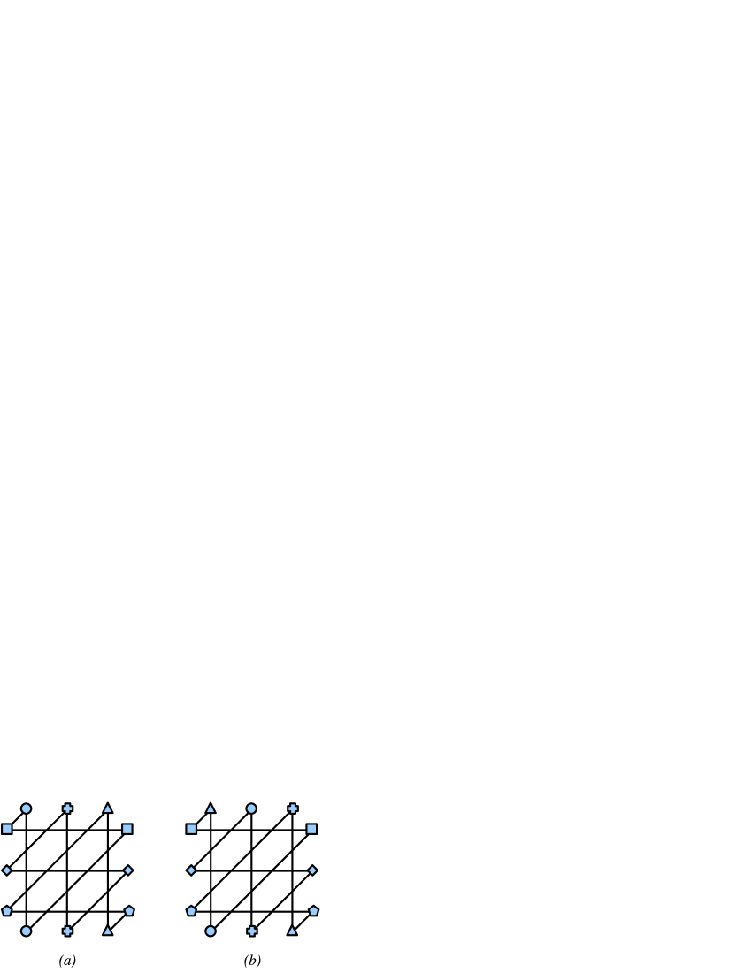
Figure 6: $3\times 3$ square bases for the kagome lattice with: a) straight embedding, b) a twisted embedding.

A variation of the straight embedding is to shift cyclically the vertices along one of the sides of the square before gluing them to those of the opposing side; we call this a twisted embedding. By reflection symmetry, shifting cyclically $k$ steps to the right or to the left produces identical results. There are thus in general $1+\lfloor n/2\rfloor$ inequivalent twists, corresponding to $k=0,1,\ldots,\lfloor n/2\rfloor$. In practice we have found that for some—but not all—lattices the cases $(n,k)=(2,0)$ and $(n,k)=(2,1)$ produce the same critical polynomial.

A square basis $B$ of size $n\times n$ has $n$ terminals on each of the four sides of the square. The number of vertices and edges in $B$ are both proportional to $n^{2}$. In the vertex count, each terminal counts for $1/2$ only, since it is shared among two copies of the basis. Thus, the square basis for the kagome lattice shown in Figure 6 has $6n^{2}$ edges and $3n^{2}$ vertices.

One can obviously generalise this construction to rectangular bases of size $n\times m$. For $n=m$ one recovers a square basis. For $n\neq m$ the twists along the $n$ and $m$ directions are no longer equivalent.

2.2.2 Hexagonal bases

When the lattice $L$ has a 3-fold rotational symmetry, one can define as well a hexagonal embedding. Examples of this are shown in Figure 7. Each of the six sides of the hexagon now supports $n$ terminals. Note that it is not possible to twist the hexagonal bases, since only the straight embedding produces a valid tiling of two-dimensional space.

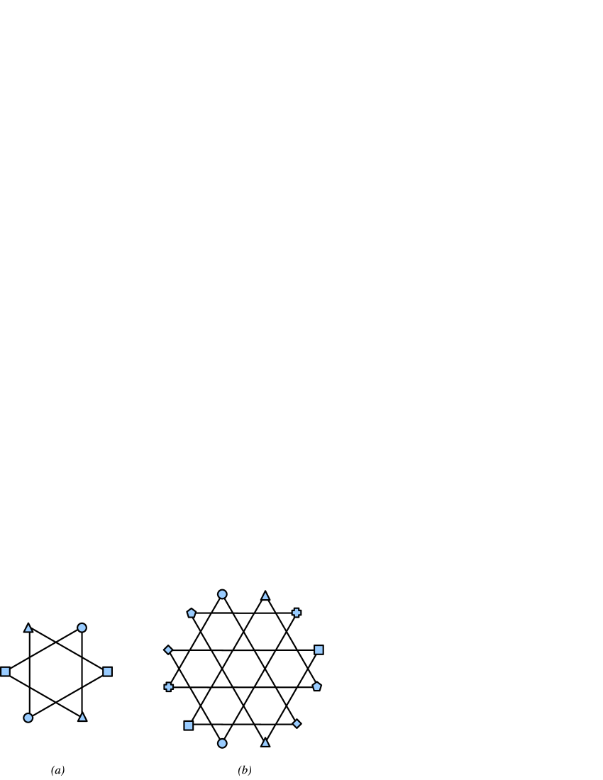
Figure 7: Hexagonal bases for the kagome lattice with a) $n=1$, and b) $n=2$.

One advantage of hexagonal bases over the square bases is that they have a lower ratio of terminals to edges, which is useful because the number of terminals is the limiting factor in the transfer matrix computation. For instance, for the kagome lattice one has now $6n$ terminals, $9n^{2}$ vertices and $18n^{2}$ edges.

Another advantage is that the hexagonal basis is designed to respect the 3-fold rotational symmetry of the lattice. Thus, for lattices having this symmetry—such as the kagome and $(3,12^{2})$ lattice—we expect the hexagonal basis to yield better accuracy than the square basis for a given number of edges. We shall come back to this point in section 4.

Note that one can extend this construction to generalised hexagonal bases with $2(n_{1}+n_{2}+n_{3})$ terminals, where each pair of opposing sides of the hexagon supports $n_{i}$ terminals $(i=1,2,3)$. The special case with one of the $n_{i}=0$ reproduces the rectangular bases.

3 Transfer matrix

The probabilities $P(2D;B)$ and $P(0D;B)$ entering the definition (6) of the critical polynomial can be computed from a transfer matrix construction along the lines of Ref. [25]. First notice that each state of the edges within the basis $B$ induces a set partition among the terminals; each part (or block) in the partition consists of a subset of terminals that are mutually connected through paths of open edges. The key idea is to first compute the probabilities of all possible partitions. One next groups the partitions according to their 2D, 1D or 0D nature in order to evaluate (6).

With $N$ terminals, the number of partitions respecting planarity is given by the Catalan number

$$C_{N}=\frac{1}{N+1}{2N\choose N}\,.$$ (10)

For example, the $C_{3}=5$ planar partitions of the set $\{1,2,3\}$ are denoted

$$(1)(2)(3)\,,\quad(12)(3)\,,\quad(13)(2)\,,\quad(1)(23)\,,\quad(123)\,,$$ (11)

where the elements belonging to the same part are grouped inside parentheses.

The dimension of the transfer matrix is thus $C_{N}$, and both time and memory requirements are proportional to this number. Asymptotically we have $C_{N}\sim 4^{N}$ for $N\gg 1$. Taking as an example the kagome lattice with the $n\times n$ square basis, the time complexity of the transfer matrix method is then $\sim 4^{4n}=2^{8n}$. This can be compared to the contraction-deletion method, whose number of recursive calls is $\sim 2^{6n^{2}}$.

3.1 Square bases

Our transfer matrix construction is most easily explained on a specific example. So consider the kagome lattice with the $n\times n$ square basis; the case $n=3$ is shown in Figure 8.

Figure 8: Transfer matrix construction for the kagome lattice on an $n\times n$ square basis, here with $n=3$. The operator ${\sf B}_{i}$ adds six edges to the lattice.

The transfer matrix ${\sf T}$ constructs the lattice from the bottom to the top, while keeping track of the Boltzmann weight of each partition of the terminals. The bottom terminals are denoted $1,2,\ldots,2n$ and the top terminals $1^{\prime},2^{\prime},\ldots,2n^{\prime}$. At the beginning of the process the top and bottom are identified, so the initial state $|{\rm i}\rangle$ on which ${\sf T}$ acts is the partition $(1\,1^{\prime})(2\,2^{\prime})\cdots(2n\,2n^{\prime})$ with weight $1$.

We now define two kinds of operators acting on a partition [27]:

• The join operator ${\sf J}_{i}$ amalgamates the parts to which the top terminals $i^{\prime}$ and $i^{\prime}+1$ belong. In particular, on partitions in which those two terminals already belong to the same part, ${\sf J}_{i}$ acts as the identity operator. Note that if some parts contain both bottom and top terminals, the action of ${\sf J}_{i}$ can also affect the connections among the bottom terminals.

• The detach operator ${\sf D}_{i}$ detaches the top terminal $i^{\prime}$ from its part and transforms it into a singleton in the partition. In particular, if that terminal was already a singleton, ${\sf D}_{i}$ acts as the identity operator.

From these two basic operators and the identity operator ${\sf I}$ we now define an operator

$${\sf H}_{i}={\sf I}+v{\sf J}_{i}$$ (12)

that adds a horizontal edge to the lattice. The word “horizontal” refers to a drawing of the lattice where the top terminals $i^{\prime}$ and $i^{\prime}+1$ are horizontally aligned; otherwise the edge would be better described as “diagonal”. Note that ${\sf H}_{i}$ attaches a weight $1$ (resp. $v$) to a closed (resp. open) horizontal edge, as required. Similarly we define

$${\sf V}_{i}=v{\sf I}+{\sf D}_{i}$$ (13)

that adds a vertical edge between $i^{\prime}$ and $i^{\prime\prime}$, where $i^{\prime}$ (resp. $i^{\prime\prime}$) denotes the corresponding top terminal before (resp. after) the action of ${\sf V}_{i}$. To simplify the notation, it is convenient to assume that following the action of ${\sf V}_{i}$ we relabel $i^{\prime\prime}$ as $i^{\prime}$. The word “vertical” refers to a drawing of the lattice where $i^{\prime}$ and $i^{\prime\prime}$ are vertically aligned.

The fundamental building block of the lattice shown on the right of Figure 8 is then constructed by the composite operator

$${\sf B}_{i}={\sf H}_{i}{\sf V}_{i}{\sf H}_{i}{\sf D}_{i+1}{\sf H}_{i}{\sf V}_{i}{\sf H}_{i}\,,\qquad\mbox{Kagome lattice.}$$ (14)

The whole lattice $B$ is finally obtained by adding successive rows (for clarity shown in alternating hues on the left of Figure 8) of ${\sf B}_{i}$. The transfer matrix then reads

$${\sf T}=\prod_{y=1}^{n-1}\prod_{x=1}^{y}{\sf B}_{n-y-1+2x}\times\prod_{y=1}^{n}\prod_{x=0}^{n-y}{\sf B}_{y+2x}$$ (15)

and the final state

$$|{\rm f}\rangle={\sf T}|{\rm i}\rangle$$ (16)

contains all possible partitions among the $4n$ terminals along with their respective Boltzmann weights.

3.1.1 Other lattices

The extension to the other lattices considered in this paper is very simple: it suffices to change the definition of the operator ${\sf B}_{i}$, while leaving the remainder of the construction unchanged.

Figure 9: Transfer matrix construction for the $(4,8^{2})$ lattice on an $n\times n$ square basis, here with $n=3$. The operator ${\sf B}_{i}$ adds six edges to the lattice.

The square basis for the $(4,8^{2})$ lattice is shown in Figure 9. Its fundamental building block now has the expression

$${\sf B}_{i}={\sf H}_{i}{\sf V}_{i}{\sf V}_{i+1}{\sf H}_{i}{\sf V}_{i}{\sf V}_{i+1}\,,\qquad\mbox{$(4,8^{2})$ lattice.}$$ (17)

Figure 10: Transfer matrix construction for the $(3,12^{2})$ lattice on an $n\times n$ square basis, here with $n=3$. The operator ${\sf B}_{i}$ adds nine edges to the lattice.

As a last example, consider the $(3,12^{2})$ lattice with the square basis depicted in Figure 10. We find in this case

$${\sf B}_{i}={\sf H}_{i}{\sf V}_{i}{\sf H}_{i}{\sf V}_{i}{\sf D}_{i+1}{\sf H}_{i}{\sf V}_{i}{\sf H}_{i}{\sf V}_{i}{\sf V}_{i+1}\,,\qquad\mbox{$(3,12^{2})$ lattice.}$$ (18)

3.2 Hexagonal bases

Because of their 3-fold rotational symmetry, it is also interesting to study the kagome and $(3,12^{2})$ lattice with a hexagonal basis. We now describe how to adapt the transfer matrix construction to this case.

Figure 11: Kagome lattice on a hexagonal basis of size $n$, here with $n=3$. The operator ${\sf B}_{i}$ adds six edges to the lattice, while the left and right boundary operators, ${\sf L}_{i}$ and ${\sf R}_{i}$, each add three.

Consider as an example the kagome lattice with the hexagonal basis of size $n$; the case $n=3$ is shown in Figure 11. There are now $6n$ terminals. Those on the two bottom sides (resp. the two top sides) of the hexagon are labelled $1,2,\ldots,2n$ (resp. $1^{\prime},2^{\prime},\ldots,2n^{\prime}$), just as in the case of the square basis. We describe below how the remaining terminals on the left and right sides of the hexagon are to be handled. The transfer matrix ${\sf T}$ still constructs the lattice from the bottom to the top.

The expression for the building block ${\sf B}_{i}$ now needs some modification, since the orientation of the bow tie motif with respect to the transfer direction (invariably upwards) has been changed. One easy option would be to handle the centre of the bow tie as an extra point—we would then label the three points $i$, $i+1$ and $i+2$)—and use the expression ${\bf B}_{i}={\sf D}_{i+1}{\sf H}_{i+1}{\sf H}_{i}{\sf V}_{i+2}{\sf V}_{i}{\sf H}_{i+1}{\sf H}_{i}$. It is however more efficient to avoid introducing the centre point into the partition (and keep the usual labelling $i$, $i+1$ as shown on the right of Figure 11). The expression for ${\sf B}_{i}$ can then be found by computing the final state (16) for the $1\times 1$ square basis and rotating the labels (we denote here $j=i+1$):

$${\sf B}_{i} = (v^{6}+6v^{5}+9v^{4})(iji^{\prime}j^{\prime})+(2v^{4}+6v^{3}+v^{2})(ii^{\prime})(jj^{\prime})$$ (19)

$$+ (v^{4}+3v^{3})\big{[}(i)(ji^{\prime}j^{\prime})+(j)(ii^{\prime}j^{\prime})+(i^{\prime})(ijj^{\prime})+(j^{\prime})(iji^{\prime})\big{]}$$

$$+ (v^{3}+5v^{2}+v)\big{[}(ii^{\prime})(j)(j^{\prime})+(i)(i^{\prime})(jj^{\prime})\big{]}+(4v+1)(i)(j)(i^{\prime})(j^{\prime})$$

$$+ v^{2}\left[(i)(j)(i^{\prime}j^{\prime})+(ij)(i^{\prime})(j^{\prime})+(i)(i^{\prime}j)(j^{\prime})+(i^{\prime})(ij^{\prime})(j)\right]\,.$$

where a bracketed operator, for example $(ii^{\prime})(jj^{\prime})$, creates a bow-tie between $i$ and $j$ with the indicated partition of its four bounding vertices. On the boundary of the hexagon we need the further operators

$${\sf L}_{i} = {\sf H}_{i}{\sf V}_{i+1}{\sf H}_{i}\,,$$ (20)

$${\sf R}_{i} = {\sf H}_{i}{\sf V}_{i}{\sf H}_{i}\,.$$ (21)

The transfer matrix that builds the whole hexagon then reads

$${\sf T} = \prod_{y=1}^{n-1}\prod_{x=1}^{y}{\sf B}_{n-y-1+2x}$$ (22)

$$\times \prod_{y=1}^{n}\left(\prod_{x=1}^{n}{\sf B}_{2x-1}\times{\sf L}_{0}\prod_{x=1}^{n-1}{\sf B}_{2x}\times R_{2n}\right)\times\prod_{y=1}^{n}\prod_{x=0}^{n-y}{\sf B}_{y+2x}\,.$$

Regarding the handling of the boundary points, a small remark is in order. In (22) these have been denoted simply $0$ (on the left) and $2n+1$ (on the right). In the initial state $|{\rm i}\rangle$, both $0$ and $2n+1$ are singletons. After each factor in the middle product over $y$ the two boundary labels have to be stored, so that in the final state (16) the partitions indeed involve all $6n$ terminals. To avoid introducing a cumbersome notation, we understand implicitly that this storing is performed when expanding the product (22).

3.2.1 Other lattices

The $(3,12^{2})$ lattice can be handled similarly by rotating ${\sf B}_{i}$ shown in the right part of Figure 10 through angle $\pi/2$ clockwise. The left (resp. right) boundary operator ${\sf L}_{i}$ (resp. ${\sf R}_{i}$) then consists of the four rightmost (resp. five leftmost) edges in the rotated ${\sf B}_{i}$.

Explicitly we find

$${\sf B}_{i} = (v^{9}+6v^{8}+9v^{7})(iji^{\prime}j^{\prime})+(v^{7}+3v^{6})\left[(iji^{\prime})(j^{\prime})+(iji^{\prime})(j)\right]$$

$$+ (v^{8}+7v^{7}+13v^{6}+3v^{5})\left[(i)(ji^{\prime}j^{\prime})+(i^{\prime})(ijj^{\prime})\right]$$

$$+ (v^{8}+8v^{7}+17v^{6}+7v^{5}+v^{4})(ii^{\prime})(jj^{\prime})$$

$$+ (3v^{6}+12v^{5}+6v^{4}+v^{3})(ii^{\prime})(j)(j^{\prime})$$

$$+ (3v^{7}+28v^{6}+77v^{5}+70v^{4}+34v^{3}+9v^{2}+v)(i)(i^{\prime})(jj^{\prime})$$

$$+ (v^{6}+4v^{5}+v^{4})\left[(i)(j)(i^{\prime}j^{\prime})+(ij)(i^{\prime})(j^{\prime})+(i)(i^{\prime}j)(j^{\prime})+(i^{\prime})(ij^{\prime})(j)\right]$$

$$+ (8v^{5}+45v^{4}+49v^{3}+27v^{2}+8v+1)(i)(j)(i^{\prime})(j^{\prime})$$

along with

$${\sf L}_{i} = (v^{4}+3v^{3})(ijj^{\prime})+(v^{3}+4v^{2}+v)(i)(jj^{\prime})$$ (24)

$$+ v^{2}\left[(ij)(j^{\prime})+(ij^{\prime})(j)\right]+(3v+1)(i)(j)(j^{\prime})$$

and

$${\sf R}_{i} = (v^{5}+3v^{4})(ii^{\prime}j)+(v^{4}+4v^{3}+v^{2})\left[(ij)(i^{\prime})+(i)(i^{\prime}j)\right]$$ (25)

$$+ v^{3}(ii^{\prime})(j)+(v^{3}+8v^{2}+5v+1)(i)(j)(i^{\prime})\,.$$

The other problem we can handle with this construction is site percolation on the hexagonal lattice. Here, a “bow-tie” consists only of two sites, which replace the triangles of the kagome lattice. Now many of the weights in the operator ${\sf B}_{i}$ are zero, as those partitions are not possible, and the remaining terms are fairly simple:

$${\sf B}_{i}=v^{2}(iji^{\prime}j^{\prime})+v\left[(ii^{\prime})(j)(j^{\prime})+(i)(i^{\prime})(jj^{\prime})\right]+1(i)(j)(i^{\prime})(j^{\prime})$$ (26)

with

$${\sf L}_{i}=v(ijj^{\prime})+1(i)(j)(j^{\prime})$$ (27)

and

$${\sf R}_{i}=v(ii^{\prime}j)+1(i)(i^{\prime})(j^{\prime})\ .$$ (28)

3.3 Distinguishing 2D, 1D and 0D partitions

We now explain how each partition entering the final state (16) can be assigned the correct homotopy (0D, 1D or 2D) in order to make possible the application of the main result (6). The definition of homotopy that we have given in section 2.1 is not very practical, because it refers to the connectivity properties between two arbitrarily separated copies of the basis, $B_{1}$ and $B_{2}$. The purpose of this section is to provide an operational determination of the homotopy using just intrinsic properties of $B$.

Each partition of the set of $N$ terminals can be represented as a planar hypergraph on $N$ vertices, where each part of size $k>1$ in the partition corresponds to a hyperedge of degree $d=k-1$ in the hypergraph. Because of the planarity we can obtain yet another representation as an ordinary graph on $2N$ vertices with precisely $N$ ordinary ($d=1$) edges. We now detail this construction, which is completely analogous to a well-known [28] equivalence for the partition function of the Potts model defined on a planar graph $G$ that can be represented, on the one hand, in terms of Fortuin-Kasteleyn clusters [29] on $G$ and, on the other hand, as a loop model on the medial graph ${\cal M}(G)$.

The hypergraph can be drawn inside the frame (the outer boundary of the shaded areas in Figures 8 and 11) on which the $N$ terminals live. Here we give a few examples:

Now place a pair of points slightly shifted on either side of each of the $N$ terminals. Draw $N$ edges between these $2N$ points by “turning around” the hyperedges and isolated vertices of the hypergraph. We shall refer to this as the surrounding graph. For each of the above examples this produces:

The embedding of $B$ is defined by identifying points on opposing sides of the frame (to produce the twisted embeddings we further shift the points on one of the sides cyclically before imposing the identification). Let $\ell$ be the number of loops in the surrounding graph. The partition is of the 1D type if and only if one or more of these loops is non-homotopic to a point. To determine whether this is the case it suffices to “follow” each loop until one comes back to the starting point, and determine whether the total signed displacement in the $x$ and $y$ directions is non-zero. Using this method one sees that the middle partition in the above three examples is of the 1D type.

If all loops on the surrounding graph have trivial homotopy, one can use the Euler relation to determine whether the partition is of the 0D or 2D type. Namely, let $E$ be the sum of all degrees of the hyperedges in the hypergraph; let $C$ (resp. $V$) be the number of connected components (resp. vertices) in the hypergraph after the identification of opposing sides. Then the combination

$$\chi=E+2C-V-\ell$$ (29)

equals 0 (resp. 2) if the partition is of the 0D (resp. 2D) type.

For instance, for the leftmost example we have $E=3+1+1=5$, $C=1$, $V=6$, and $\ell=1$, whence $\chi=0$. And for the rightmost example one finds $E=5+1=6$, $C=2$, $V=6$, and $\ell=2$, whence $\chi=2$.

4 Bond percolation

In this section we present our results for bond percolation. The actual critical polynomials are very large polynomials of degree up to 243 with very large integer coefficients (more than 40 digits), and thus it does not seem reasonable to make them appear in print. As a compromise, all the polynomials are collected in the text file SC12.m which is available in electronic form as supplementary material to this paper. The printed version contains only the relevant zeros $p_{c}\in[0,1]$, rounded to 15 digit numerical precision.

4.1 Kagome lattice

The bond percolation threshold of the kagome lattice is perhaps the most studied of the unknown bond critical probabilities. Non-rigourous conjectures [16, 30] and approximations [14] have appeared in the literature, as well as rigourous bounds [31] and confidence intervals [32]. To compute polynomials on the kagome lattice, we considered two families of bases: square (see section 2.2.1) and hexagonal (see section 2.2.2).

4.1.1 Square bases

The $n\times n$ square bases with straight and twisted embeddings are shown in Figure 6. They contain $3n^{2}$ vertices and $6n^{2}$ edges. The percolation thresholds $p_{c}$ obtained for $n\leq 4$ and twist $k\leq\lfloor n/2\rfloor$ are given in Table 1. Note that the results for $(n,k)=(2,0)$ and $(2,1)$ are identical for this lattice; but otherwise the critical polynomial does depend on $k$.

For the largest ($n=4$) basis, containing $96$ edges, the results for $p_{c}$ with the three possible twists have the same first $8$ digits, perhaps suggesting that at least the first $7$ are actually correct. By comparing the entries, it also appears that, at least for $n<4$, the thresholds are correct to the first $n+3$ digits. The numerical results of Feng, Deng, and Blöte [33] place the bond threshold at $p_{c}=0.524\,404\,99(2)$ using a transfer matrix approach, and $p_{c}=0.524\,405\,03(5)$ with Monte Carlo. Our value is within the error of their second result and can hardly be considered definitively ruled out by their first. Of course, we cannot hope that our result is exact, because, as shown in [10], no basis of finite size will ever yield the exact answer.

$n$	twist	$p_{c}$
1	0	0.524 429 717 521 275
2	0	0.524 406 723 188 232
	1	0.524 406 723 188 232
3	0	0.524 405 172 713 770
	1	0.524 405 153 253 058
4	0	0.524 405 027 427 415
	1	0.524 405 026 221 984
	2	0.524 405 020 086 919

Table 1: Bond percolation predictions for the kagome lattice on the $n\times n$ square bases with various twists.

4.1.2 Hexagonal bases

The hexagonal bases of size $n$ are shown in Figure 7. They contain $9n^{2}$ vertices and $18n^{2}$ edges. As discussed in section 2.2.2 these bases better respect the rotational symmetry of the lattice, and hence we expect the results to be more precise than those with the square bases for a given number of edges. Results for $n\leq 3$  are given in Table 2.

We also note that our $p_{c}$ for $n\times n$ square bases (1) are monotonically decreasing with $n$, while those with hexagonal bases are increasing. If these trends hold as $n\rightarrow\infty$, then the kagome threshold satisfies

$$0.524\,404\,998\,266\,288<p_{c}<0.524\,405\,020\,086\,919\ .$$ (30)

While this is much more stringent than Wierman’s bounds [31],

$$0.5209<p_{c}<0.5291$$ (31)

his result is completely rigourous while ours is only a guess based on the observed monotonicity in the estimates with $n$. In fact, as we will soon see, the $(3,12^{2})$ lattice violates this monotonicity for the $n=3$ hexagonal basis, making (30) even less certain. Nevertheless, the kagome $n=2$ and $3$ (i.e., $72$ and $162$ edges) predictions appear to be converged to at least seven digits, and agree with the transfer matrix result $p_{c}=0.524\,404\,99(2)$ of Feng, Deng, and Blöte [33] to eight decimal places (the limit of their accuracy). Thus we can cautiously conclude that the true bond threshold is

$$p_{c}=0.524\,405\,00(1)\,,\qquad\mbox{Kagome lattice.}$$ (32)

More recently, Ding et. al. [13] reported $p_{c}=0.524\,404\,978(5)$; our results and those of [33] seem to agree that the error bar of these authors might be slightly underestimated.

$n$	$p_{c}$
1	0.524 403 641 312 579
2	0.524 404 993 638 028
3	0.524 404 998 266 288

Table 2: Bond percolation predictions for the kagome lattice on the $n$–sided hexagonal bases.

4.2 $(4,8^{2})$ lattice

We computed the critical polynomials for the $n\times n$ square bases on the $(4,8^{2})$ lattice (see Figure 12). As this graph does not have the kagome lattice’s hexagonal symmetry, there are no corresponding hexagonal bases. Results for $n\leq 4$ are given in Table 3, with the twists $k\leq\lfloor n/2\rfloor$ defined identically to the kagome case. Note that the cases $(n,k)=(2,0)$ and $(2,1)$ now produce different results.

The bond threshold of this lattice has not been studied as thoroughly as that of the kagome lattice, and apparently the only high-precision result is Parviainen’s [11], $p_{c}=0.676\,802\,32(63)$. Our $4\times 4$ results are within two standard deviations.

$n$	twist	$p_{c}$
1	0	0.676 835 198 816 406
2	0	0.676 811 051 133 795
	1	0.676 805 751 049 826
3	0	0.676 805 010 886 365
	1	0.676 803 989 559 125
4	0	0.676 803 693 656 055
	1	0.676 803 476 910 363
	2	0.676 803 329 691 626

Table 3: Bond percolation predictions for the $(4,8^{2})$ lattice on the $n\times n$ square bases with various twists.

Figure 12: The $3\times 3$ square basis, with unspecified embedding, for the $(4,8^{2})$ lattice.

4.3 $(3,12^{2})$ lattice

The $(3,12^{2})$ lattice bears more than a passing resemblance to the kagome lattice. Employing the analogous $n\times n$ square bases and twists, we find the results in Table 4.

$n$	twist	$p_{c}$
1	0	0.740 423 317 919 897
2	0	0.740 420 992 429 996
	1	0.740 420 992 429 996
3	0	0.740 420 818 821 979
	1	0.740 420 817 594 340
4	0	0.740 420 802 130 112
	1	0.740 420 802 158 172
	2	0.740 420 801 695 085

Table 4: Bond percolation predictions for the $(3,12^{2})$ lattice on the $n\times n$ square bases with various twists.

Like the kagome lattice, the bond threshold on this lattice has been studied extensively. Parviainen, using simulations, gives the threshold as $p_{c}=0.740\,421\,95(80)$. More recent transfer matrix work by Ding et al. [13] gives $p_{c}=0.740\,420\,77(2)$, whereas Ziff and Gu [12] report $p_{c}=0.740\,420\,81(10)$ based on a fitting method.

$n$	$p_{c}$
1	0.740 420 702 159 477
2	0.740 420 799 397 205
3	0.740 420 798 850 745

Table 5: Bond percolation predictions for the $(3,12^{2})$ lattice on the hexagonal bases of side $n$.

Results with the hexagonal basis are shown in Table 5. While the square basis values seem to approach the exact solution from above, as in the kagome case, the hexagonal bases deviate from the trend of approach from below with the $n=3$ result. Nevertheless, it is this latter estimate that we expect to be the most accurate, and we cautiously conclude that the true bond threshold of $(3,12^{2})$ is

$$p_{c}=0.740\,420\,800(2)\,,\qquad\mbox{$(3,12^{2})$ lattice.}$$ (33)

This value is one order of magnitude more precise than the most recent numerical work and demonstrates the potential of the critical polynomials for determining high-precision critical thresholds.

5 Site percolation

The condition (6) allows for a straightforward extension to site percolation. We first demonstrate that the results for the smallest possible bases correctly retrieve the thresholds for exactly solvable lattices. We then present results with large bases for the square and hexagonal lattices.

5.1 Exactly solvable lattices

In some sense, site percolation is more fundamental than the bond problem. This is because every lattice has a line graph, or covering lattice, which maps bond percolation to a corresponding site problem. The covering lattice of $L$ is formed by placing a vertex on every edge of $L$, and drawing edges between vertices that cover adjacent edges of $L$. The resulting graph is usually not planar, but it is obvious that site percolation on the covering lattice is identical to bond percolation on $L$. The inverse construction is rarely possible. That is, not every site problem can be mapped to a bond problem (without resorting to hyperedges) on an underlying $L$, and in this sense bond percolation is a special case of the site problem. Although there are now lattices for which the site thresholds are known that are neither self-matching nor the covering lattices of bond problems [8, 7], among the Archimedean lattices only the triangular, which is self-matching and thus has $p_{c}^{\mathrm{site}}=1/2$, and the kagome and $(3,12^{2})$ lattices, which are the line graphs of the hexagonal and doubled-bond hexagonal lattices respectively, have known site thresholds. Here, we apply the method to these solvable cases to verify that the condition (6) does reproduce exact solutions.

5.1.1 Triangular lattice

Site percolation configurations on the triangular lattice can be conveniently described as colourings of the faces on the dual, hexagonal lattice. The simplest possible basis $B$ consists of just a single hexagon, for which we use the hexagonal embedding. Clearly $P(2D;B)=v$ and $P(0D;B)=1$, so that (6) yields $v_{c}=1$ or $p_{c}=1/2$, which is indeed the correct answer.

5.1.2 Kagome and $(3,12^{2})$ lattices

For the kagome lattice we similarly consider face colourings of the dual, diced lattice, which is a tiling of the plane with three differently oriented lozenges. The simplest basis $B$ consists of three different lozenges inscribed in a hexagon. We have then $P(2D;B)=v^{3}$, $P(1D;B)=3v^{2}$, and $P(0D;B)=3v+1$. Application of (6) then gives the critical polynomial

$$1-3p^{2}+p^{3}=0\,,$$ (34)

and the relevant zero $p_{c}=1-2\sin(\pi/18)=0.652\,704\cdots$ provides the exactly known threshold.

A very similar computation for the $(3,12^{2})$ lattice, using a basis of six sites, gives the same answer as for the kagome lattice, except that $p$ is replaced by $p^{2}$.

5.2 Square lattice

For the square lattice we use rectangular bases of $n\times m$ sites (see section 2.2.1). The site polynomials on this lattice are not found any more efficiently with the transfer matrix of section 3 than by simply using the brute force approach of generating all $2^{nm}$ configurations and directly computing the probabilities $P(2D)$ and $P(0D)$. Therefore we take the latter approach in this case. The results for $n,m\leq 6$ are shown in Table 6.

basis	$p_{c}$
$1\times 1$	0.5
$2\times 2$	0.541 196 100 146 197
$3\times 3$	0.586 511 455 112 676
$3\times 4$	0.588 361 985 284 352
$4\times 4$	0.590 672 112 331 028
$4\times 5$	0.591 269 973 846 402
$5\times 5$	0.591 988 256 518 334
$5\times 6$	0.592 167 665 055 742
$6\times 6$	0.592 395 070 817 704

Table 6: Site percolation predictions for the square lattice on $n\times m$ rectangular bases.

The site threshold on the square lattice is the subject of perhaps the most numerical studies of all the Archimedean percolation problems [33, 34, 35, 36, 37, 38, 39]. To take the most recent of these, Lee [39] found $p_{c}=0.592\,745\,98(4)$ by a Monte Carlo scheme, whereas Feng, Deng and Blöte [33] used both Monte Carlo, $p_{c}=0.592\,746\,06(5)$, and transfer matrix, $p_{c}=0.592\,746\,05(3)$, methods. These results are all within each other’s error bars and unanimously and decisively rule out our best polynomial prediction. Compared with the bond percolation results presented here, it is striking how poorly the polynomials perform for this problem. Even for the $36^{\mathrm{th}}$-order polynomial of the $6\times 6$ basis, we are left with a prediction that is barely within $3.5\times 10^{-4}$ of the numerical answer, whereas a polynomial for a bond problem is typically off by only $10^{-7}$ at this order [4, 10].

5.3 Hexagonal lattice

Although the bond percolation threshold for the hexagonal lattice has been known rigourously for a long time [40], and conjecturally for even longer [17], its exact site threshold remains elusive. Before accurate numerical results were available, it was guessed, based on a star-triangle argument, that the site threshold is given by $p_{c}=1/\sqrt{2}\approx 0.707107$ [41]. Although this is now known to be incorrect, it is reasonably close and in fact, the critical polynomial for the two-site basis also makes this prediction. We improve upon this estimate by employing the hexagonal bases of Figure 7 with each triangle of the kagome lattice replaced with a site (the kagome lattice is the medial graph of the hexagonal) and the transfer operators B, L and R given by (26)–(28).

Predictions for $n=1$, $2$ and $3$ (for $n=3$, a parallel computation was necessary, utilizing $2046$ processors, which completed in about three hours), are roots of $6^{\mathrm{th}}$, $24^{\mathrm{th}}$, and $54^{\mathrm{th}}$ order polynomials. These thresholds are presented in Table 7. Suding and Ziff’s Monte Carlo estimate [42] places the critical probability around $p_{c}=0.697\,043(3)$. A more recent transfer matrix result of Feng, Deng, and Blöte [33] is $p_{c}=0.6970402(1)$, and, although it is within $2.6\times 10^{-6}$, our $n=3$ prediction is clearly ruled out. This is in sharp contrast to the bond results for the kagome and $(3,12^{2})$ lattices, which already challenge the numerical results at $n=2$. However, this is still better than the situation for site percolation on the square lattice. The $n=2$ hexagonal basis contains $24$ sites and makes a prediction within $2.2\times 10^{-5}$ of the numerical value, which is an order of magnitude better than the $36$–site square lattice basis. We will have more to say about this below.

$n$	$p_{c}$
$1$	0.691 538 728 617 958
$2$	0.697 018 214 522 145
$3$	0.697 037 409 746 762

Table 7: Site percolation predictions for the hexagonal lattice on hexagonal bases of side length $n$.

6 Discussion

In this work, we have given a re-definition, equation (6), of the generalised critical polynomial which was defined previously through contraction-deletion. While the old definition placed a practical limit on the computation of polynomials of about $36^{\mathrm{th}}$ order, this new definition allowed us to use a transfer matrix approach to calculate polynomials up to degree $243$. The results presented here provide very clear evidence for the conjecture, put forward, for example, in [3] and [5], that the root in $[0,1]$ of a generalised critical polynomial, $P_{B}(p)$, provides either the exact percolation threshold, or gives an approximation that approaches the exact answer in the limit of an appropriately infinite basis $B_{\infty}$. Specifically, it was conjectured in [5] that, as long as the aspect ratio of the limiting $B_{\infty}$ is non-zero and finite, then all possible $B_{\infty}$ make the same prediction for the critical probability. We have provided evidence for this as well, through the use of both square and hexagonal bases for the kagome and $(3,12^{2})$ lattices.

Needless to say, there is a fair degree of conjecture involved in this work. First of all, the equivalence between the contraction-deletion definition and the probabilistic definition (6) of the polynomials, which we found essentially by inspection, needs to be firmly established. Furthermore, the central idea behind all our computations, namely that (6) fixes the critical point in the scaling limit, follows from universality and so is possibly very difficult to prove in general. Even granted universality, it is not clear why this toroidal crossing probability should be the one that provides the most rapid passage into the scaling limit, at least as far as the critical threshold is concerned. Nevertheless, all these things appear to be true, as we hope we have demonstrated, and, even absent the wanted rigour, this method produces very accurate thresholds and may even come to supplant other numerical techniques for determining critical probabilities, at least for bond problems.

The kagome and $(3,12^{2})$ bond results seemingly cannot be ruled out by current numerics, but the square site and hexagonal predictions are not as competitive. The method seems to perform best for families of bases in which the ratio, which we denote $\zeta(n)$, of the number of boundary vertices, or terminals, to the number of internal elements (sites or bonds) is large. The hexagonal bases of side $n$ have $6n$ terminals, but the number of interior elements depends on the lattice chosen. For the hexagonal site problem, there are $6n^{2}$ sites so $\zeta(n)=1/n$, for kagome bond percolation $\zeta(n)=1/(3n)$, while for $(3,12^{2})$ $\zeta(n)=2/(9n)$. Even at $n=2$, the latter two problems make predictions comparable to numerics, whereas the $n=3$ hexagonal site prediction is ruled out, and it is tempting to believe that the speed with which the estimates approach the exact answer is related to the speed with with $\zeta(n)$ goes to $0$ as $n\rightarrow\infty$. Further support for this is found by considering the square site problem, in which the square bases have $4n$ terminals and $n^{2}$ sites, or $\zeta(n)=4/n$, so the worst estimates are given by the system with the slowest convergence of $\zeta(n)$ to $0$.

There are many other directions for future work. The condition (6) has a generalization to the $q-$state Potts model, allowing predictions of critical points for general $q$ of similar quality to those reported here for $q=1$. This is the subject of ongoing study. Also, the general strategy employed here may be applicable to other lattice models, for which exact results are known only on some lattices. Finally, we mention that the generalised critical polynomial can be defined through contraction-deletion in higher dimensions, but it is not yet clear whether they provide any useful information about the critical point, or whether there is a higher-dimensional equivalent of equation (6).

References

References

- [1] S. R. Broadbent and J. M. Hammersley. Proc. Camb. Phil. Soc., 53:629, 1957.
- [2] C. R. Scullard and R. M. Ziff. J. Stat. Mech., P03021, 2010.
- [3] C. R. Scullard. J. Stat. Mech., P09022, 2011.
- [4] C. R. Scullard. arXiv:1207.3340.
- [5] J. L. Jacobsen and C. R. Scullard. arXiv:1204.0622.
- [6] R. M. Ziff and C. R. Scullard. J. Phys. A: Math. Gen., 39:15083, 2006.
- [7] R. M. Ziff. Phys. Rev. E, 73:016134, 2006.
- [8] C. R. Scullard. Phys. Rev. E, 73:016107, 2006.
- [9] B. Bollobás and O. Riordan. In An Irregular Mind, volume 21 of Bolyai Society Mathematical Studies, pages 131–217. Springer Berlin Heidelberg, 2010.
- [10] C. R. Scullard. arXiv:1111.1061.
- [11] R. Parviainen. J. Phys. A: Math. Gen., 40:9253, 2007.
- [12] R. M. Ziff and H. Gu. Phys. Rev. E, 79:020102, 2009.
- [13] C. Ding, Z. Fu, W. Guo, and F. Y. Wu. Phys. Rev. E, 81:061111, 2010.
- [14] C. R. Scullard and R. M. Ziff. Phys. Rev. E, 73:045102(R), 2006.
- [15] W. D. May and J. C. Wierman. Combin. Probab. Comput., 16:285, 2006.
- [16] C. Tsallis. J. Phys. C: Solid State Phys., 15:L757, 1982.
- [17] M. F. Sykes and J. W. Essam. J. Math. Phys., 5:1117, 1964.
- [18] P. di Francesco, H. Saleur, and J. B. Zuber. J. Stat. Phys., 49:57, 1987.
- [19] H. T. Pinson. J. Stat. Phys., 75:1167, 1994.
- [20] R. M. Ziff, C. D. Lorenz, and P. Kleban. Physica A, 266:17, 1999.
- [21] A. Morin-Duchesne and Y. Saint-Aubin. Phys. Rev. E, 80:021130, 2009.
- [22] J. L. Cardy. J. Phys. A: Math. Gen., 25:L201, 1992.
- [23] S. Smirnov. C. R. Acad. Sci. Paris Sr. I Math., 333:239, 2001.
- [24] E. Lapalme and Y. Saint-Aubin. J. Phys. A: Math. Gen., 34:1825, 2001.
- [25] H. W. J. Blöte and M. P. Nightingale. Physica A, 112:701, 1982.
- [26] J. L. Jacobsen and J. Cardy. Nucl. Phys. B, 515:701, 1998.
- [27] J. Salas and A. D. Sokal. J. Stat. Phys., 104:609, 2001.
- [28] R. J. Baxter, S. B. Kelland, and F. Y. Wu. J. Phys. A: Math. Gen., 9:397.
- [29] C. M. Fortuin and P. W. Kasteleyn. Physica, 57:536, 1972.
- [30] F. Y. Wu. J. Phys. C, 12:L645, 1979.
- [31] J. C. Wierman. Combin. Probab. Comput., 12:95–111, 2003.
- [32] O. Riordan and M. Walters. Phys. Rev. E, 76:11110, 2007.
- [33] X. Feng, Y. Deng, and H. W. J. Blöte. Phys. Rev. E, 78:031136, 2008.
- [34] R. M. Ziff. Phys. Rev. Lett., 69:2670, 1992.
- [35] M. E. J. Newman and R. M. Ziff. Phys. Rev. Lett., 85:4104, 2000.
- [36] M. E. J. Newman and R. M. Ziff. Phys. Rev. E, 66:016129, 2002.
- [37] Y. Deng and H. W. J. Blöte. Phys. Rev. E, 72:016126, 2005.
- [38] M. J. Lee. Phys. Rev. E, 76:027702, 2007.
- [39] M. J. Lee. Phys. Rev. E, 78:031131, 2008.
- [40] J. C. Wierman. Adv. Appl. Prob., 13:298, 1981.
- [41] I. Kondor. J. Phys. C: Solid State Phys., 13:L531.
- [42] P. N. Suding and R. M. Ziff. Phys. Rev. E, 60:275, 1999.