On spatial selectivity and prediction across conditions with fMRI

Abstract

Researchers in functional neuroimaging mostly use activation coordinates to formulate their hypotheses. Instead, we propose to use the full statistical images to define regions of interest (ROIs). This paper presents two machine learning approaches, transfer learning and selection transfer, that are compared upon their ability to identify the common patterns between brain activation maps related to two functional tasks. We provide some preliminary quantification of these similarities, and show that selection transfer makes it possible to set a spatial scale yielding ROIs that are more specific to the context of interest than with transfer learning. In particular, selection transfer outlines well known regions such as the Visual Word Form Area when discriminating between different visual tasks.

I Introduction

Functional neuroimaging data are currently routinely used to better understand cognitive processes. They rely heavily on previous findings to formulate hypotheses and narrow the search space to regions of interest (ROIs), most often reported as coordinates of activation peaks [1], or from coordinate databases such as BrainMap [2]. However, understanding the literature is increasingly difficult, so that there is a need for more systematic methods, which use the images themselves to characterize the functional specificity of brain regions [3]. Transfer learning is a method that trains a classifier to learn a discriminant model on a source task, and then generalizes on a target task without further training. It can yield insights on some brain mechanisms if the tasks share specific common effects in some brain regions [4]. The goal of this work is to investigate the power of transfer learning procedures applied to pairs of cognitive contrasts, where the discrimination ability of the classifier quantifies the information shared between brain maps, and thus characterizes at which spatial scale functional contrasts can be jointly classified. We show that in many cases, transfer learning gives poor results in terms of spatial selectivity. To address this limitation, we introduce selection transfer, i.e. classification of brain states on the target task following the canonical procedure [5], but using regions defined on the source task.

II Methods

Problem setting

We start from a database holding several studies, each of them containing different functional contrast images, acquired over multiple subjects. We consider two sets of tasks, the source tasks and the target tasks, each composed of pairs of contrast images. Given $n$ contrasts pairs of $k$ voxel each, we call $\bm{X}\in\mathbb{R}^{n,k}$ the images of the source tasks, and $\bm{y}$ the label denoting the functional contrast under study. The target images and labels are defined likewise: $\bm{X}^{\star}\in\mathbb{R}^{n,k}$ and $\bm{y}^{\star}$. The source and the target share a similar functional spatial pattern, and we are interested in finding the common ROIs, as well as the differences, using a machine learning approach. Note that a common pitfall in neuroimaging classification-based data processing is a successful prediction cannot guarantee that the information used by the classifier is specific to the cognitive process of interest.

Regions selection

Feature selection is an important step of brain activity decoding procedures. Full brain decoding approaches are efficient but require a careful methodology to recover the contribution of different brain regions in the classification. To test the involvement of a particular brain region, researchers typically use ROIs from an atlas, or derived from the literature. Another option is to use methods such as the searchlight algorithm, in order to evaluate and extract spatially relevant voxels across the whole brain [6]. We choose to use a one-way ANOVA procedure [7], that yields a selection based on the functional activations elicited by a task, rather than using purely spatial information. We consider different fractions of the brain voxels that are most correlated to the functional contrast and perform the learning procedure on these voxels. We vary the percentiles of selected voxels with a cubic scale, from roughly 150 voxels to the full brain. This way we can control the spatial specificity against the prediction performance, and attempt to find an optimal set of regions.

Transfer learning

This consists in learning discriminative models on a source functional task $(\bm{X},\bm{y})$ in order to capture information that should be predictive for a target task $(\bm{X^{\star}},\bm{y^{\star}})$. The general assumption is that if a transfer occurs, the two experiments share at least some common cognitive circuity. Here, we train a linear classifier on the source task, and we predict the labels of the target without any additional training. The features are selected with a one-way ANOVA on the source task, which makes it possible to compare region-based transfer learning with full brain transfer learning.

Selection transfer

This consists in building a predictive model for the target task based on information extracted from the source task. However, here the transfer occurs on feature selection: we perform the ANOVA procedure on $(\bm{X},\bm{y})$ to select the most relevant voxels, then we train a linear classifier on $(\bm{X^{\star}},\bm{y^{\star}})$, and predict on the same task with the voxels selected from the source. Consequently, the transfer is not a generalization of a classifier as in transfer learning, but rather an evaluation of the significance of features from a task to another. We use the same linear classifier as the one used for transfer learning.

III Experiments and Results

III-A FRMI dataset

We use data from two fMRI studies for this work. The first one [8] is composed of 322 subjects and was designed to assess the inter-subject variability in some language, visual, calculation, and sensorimotor tasks. The second study is similar to the first one in terms of stimuli, but the data were acquired on 35 pairs of twin subjects. The two studies were pre-processed and analyzed with the standard fMRI analysis software SPM5. The data used for this work are a subset of the 90 different statistical images resulting from the intra-subject analyses. The raw images were acquired on a 3T SIEMENS Trio and a 3T Brucker scanner for the first study, and on a 1.5T GE Signa for the second one. Table I presents the list of contrasts pairs used for this analysis.

Contrasts Names	Selected Scale		Area under p-curve		Description
	trans.	sel.	trans.	sel.
house/scramble $\rightarrow$ face/scramble	68.11	3.25	22.73	4.51	house/scramble = house image versus scrambled image
face/scramble $\rightarrow$ house/scramble	0.40	2.67	16.22	2.71	face/scramble = face image versus scrambled image
word/scramble $\rightarrow$ face/scramble	23.77	4.63	10.36	2.88	word/scramble = word image versus scrambled image
face/scramble $\rightarrow$ word/scramble	1.36	0.79	11.15	2.29	face/scramble = face image versus scrambled image
French/sound $\rightarrow$ Korean/sound	0.40	0.02	3.57	4.61	French/sound = French listening versus unstructured sound
Korean/sound $\rightarrow$ French/sound	0.27	0.00	14.59	1.21	Korean/sound = Korean listening versus unstructured sound
V comp./sent. $\rightarrow$ A comp./sent.	11.01	0.00	2.62	1.76	V comp./sent. = computation versus sentences reading
A comp./sent. $\rightarrow$ V comp./sent.	0.01	6.36	4.75	3.10	A comp./sent. = computation versus sentences listening
V motor/sent. $\rightarrow$ A motor/sent.	0.10	0.00	11.84	1.85	V motor/sent. = button press action versus sentences reading
A motor/sent. $\rightarrow$ V motor/sent.	7.37	0.00	4.45	2.11	A motor/sent. = button press action versus sentences listening

TABLE I: Source and target tasks: Selected scales and area under the p-values curve for both transfer learning and selection transfer. trans.= transfer learning; sel.= selection transfer; V= visual stimuli; A= auditory stimuli.

III-B Experimental results for transfer learning

We are interested in transfer learning: we learn a discriminative model on the source task with a univariate feature selection, and predict the labels on the target task.

The analysis presents two phases: we first train a linear classifier on a source task, and then re-use the discriminative model on the target task to perform the transfer learning; this is repeated on 6 different sub-samples of the source task to estimate the uncertainty on transfer accuracy. We use two kinds of linear classifiers: a SVC (Support Vector Classifier) and a Logistic Regression with $\ell_{2}$ penalization. The penalization is set by nested 6-fold cross-validation for each classifier. We find that the two methods yield very close results, and thus report only results using the SVC classifier. We also train and then test the classifier on the target task and call this procedure inline learning. In Figure 1, we show the performance $\tau^{t}_{p}$ of transfer learning, relative to inline learning $\tau^{i}_{p}$, varying the percentile $p$ of features selected in a cubic scale. In general, for any given $p$, $\tau^{i}_{p}$ can remain significantly higher than $\tau^{t}_{p}$. For this reason, we use a heuristic to select the scale parameter (see also Figure 1): the scale that yields the minimal $\tau^{i}_{p}-\tau^{t}_{p}$ difference. We consider that at this scale, the maps associated with the two tasks share a maximal amount of common information.

However, the voxels selected with this method are either too few to give an accurate prediction, or too many to yield identifiable regions. The transfers do not behave the same way on both directions: in general, one direction is more sensitive but less specific, and the other direction shows the opposite behaviour. This comes from tasks-related foci being more spatially focused for some contrasts. Because of this lack of specificity, we do not find contained regions that overlap with the Fusiform Face Area (FFA) [9], the Parahippocampal Place Area (PPA) [10] or the Visual Word Form Area (VWFA) [11], regions respectively involved in face recognition, object visual processing, and reading.

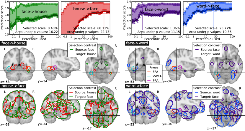
Figure 1: Example of results using the Transfer learning approach, in four different transfer settings: we can see that the area between the inner transfer prediction accuracy curves are large, and that the prediction rates do not converge. The optimal scale, defined as the minimum of the difference between the curves, often corresponds to a rather broad, non-specific brain map.

III-C Experimental results for selection transfer

We are interested in selection transfer: we do not perform transfer learning, instead, we use the univariate feature selection performed on the source task, to learn a discriminative model and predict the labels in the target task.

We use the same machine learning tools as the transfer learning: we train and test a linear classifier with a 6-fold cross validation test on the target task. For this method the SVC and the Logistic Regression with $\ell_{2}$ penalization also give very close results. As with transfer learning, we also perform an inline learning on the target task, with features selected on the same images.

On Figure 2, we show the performance $\tau^{s}_{p}$ of selection transfer against inline learning $\tau^{i}_{p}$, and how the performance varies with the percentile $p$ of the brain recruited for the learning process. In comparison to transfer learning, two things happen: i) the selection transfer is more symmetric, ii) $\tau^{i}_{p}$ is not significantly higher than $\tau^{s}_{p}$ for every $p$. We can therefore use a t-test to define the selected scale (Figure 2) as the first one with non significant difference between the curves. This enables us to control the amount of information to include in the prediction problem, and have both a good performance and an improved specificity of the regions selected for the two tasks. In practical terms, the selected scale makes it possible to identify the smallest fraction of the brain that yields overlapping regions in the two tasks, and consequently an accurate prediction. Although the selected regions have no guarantee of optimality, they are specific enough to overlap with the FFA, the PPA and the VWFA. We can also use the area under the p-values curve from the t-test as a measure of similarity between the tasks. While, it is not possible to interpret this measure absolutely, we can use it to compare one task versus others. For the example on Figure 2, we can see that the area between face and word is smaller than between face and house. This indicates that the face task is closer to the word task than the house task, which is consistent with previous findings [12].

Limitations

Selection transfer captures voxels that generalize well in terms of prediction from one task to another. However, a classifier may require very few voxels to perform well, in which case this method misses some regions involved in the cognitive process of interest. This effect is represented by the values in Table I, where selection transfer requires only a small $p$ fraction of the brain to obtain a $\tau^{s}_{p}$, which is not significantly lower than $\tau^{i}_{p}$ (e.g., V comp./sent $\rightarrow$ A motor/sent.). In order to retrieve optimal regions when this is the case, a standard analysis, based either on contrast addition or conjunction [13], would be sensitive enough to detect the common active regions for both tasks.

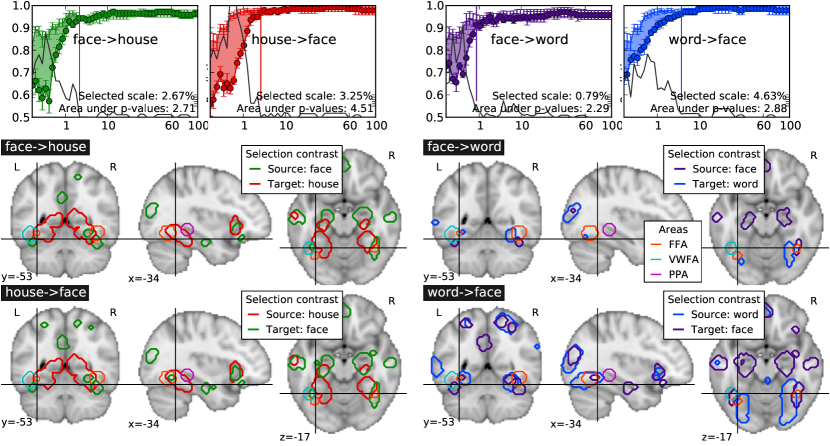
Figure 2: Example of result using the Selection transfer approach: The two prediction curves do converge, so that the difference becomes non-significant as soon as a relatively small fraction of the voxels are included: the spatial scale is defined here as the point where the curves can no longer be distinguished. It corresponds to more symmetric and meaningful brain maps than those obtained with transfer learning.

IV Conclusion

In this contribution, we investigate the ability of transfer learning and selection transfer to characterize the spatial scale at which functional contrasts can be jointly classified. The objective is to find a systematic procedure to extract ROIs that define common information between two functional tasks, instead of relying on activation coordinates from the literature. We show that transfer learning does not provide control on the regions size it uses to classify the tasks. Instead we use a selection transfer procedure that seems to better characterize which fraction of the brain yields discriminant information. Our results suggest that transfer learning requires to be used in a carefully designed study, as it is difficult to control the spatial selectivity of this method. Another interesting result is that selection transfer is not symmetric (i.e., source and target tasks are not inversible), as opposed to contrast conjunction. In the future, we would like use such methods in meta-analysis, in order to leverage large databases of functional images.

V Acknowledgements

This work was supported by the ANR grants BrainPedia ANR-10-JCJC 1408-01 and IRMGroup ANR-10-BLAN-0126-02.

References

- [1] T. Yarkoni, R. Poldrack, T. Nichols, D. Van Essen, and T. Wager, “Large-scale automated synthesis of human functional neuroimaging data,” Nature methods, vol. 8, p. 665, 2011.
- [2] A. Laird, J. Lancaster, and P. Fox, “Brainmap,” Neuroinformatics, vol. 3, p. 65, 2005.
- [3] A. Sutton, K. Abrams, and D. Jones, “Methods for meta-analysis in medical research,” John Wiley, 2000.
- [4] A. Knops, B. Thirion, E. M. Hubbard, V. Michel, and S. Dehaene, “Recruitment of an area involved in eye movements during mental arithmetic.” Science, vol. 324, p. 1583, 2009.
- [5] J. Mourão-Miranda, A. L. Bokde, C. Born, H. Hampel, and M. Stetter, “Classifying brain states and determining the discriminating activation patterns: Support vector machine on functional MRI data,” NeuroImage, vol. 28, p. 980, 2005.
- [6] N. Kriegeskorte, R. Goebel, and P. Bandettini, “Information-based functional brain mapping.” Proc Ntl Acad Sci, vol. 103, no. 10, p. 3863, 2006.
- [7] D. D. Cox and R. L. Savoy, “Functional magnetic resonance imaging (fMRI) ”brain reading”: detecting and classifying distributed patterns of fMRI activity in human visual cortex.” Neuroimage, vol. 19, p. 261, 2003.
- [8] P. Pinel, B. Thirion, S. Meriaux, A. Jobert, J. Serres, D. Le Bihan, J. Poline, and S. Dehaene, “Fast reproducible identification and large-scale databasing of individual functional cognitive networks,” BMC neuroscience, vol. 8, p. 91, 2007.
- [9] N. Kanwisher, J. McDermott, and M. Chun, “The fusiform face area: a module in human extrastriate cortex specialized for face perception,” J. Neurosci., vol. 17, p. 4302, 1997.
- [10] R. Epstein and N. Kanwisher, “A cortical representation of the local visual environment.” Nature, vol. 392, p. 598, 1998.
- [11] L. Cohen and S. Dehaene, “Specialization within the ventral stream: the case for the visual word form area.” NeuroImage, vol. 22, p. 466, 2004.
- [12] S. Dehaene, F. Pegado, L. W. Braga et al., “How learning to read changes the cortical networks for vision and language.” Science, vol. 330, p. 1359, 2010.
- [13] T. Nichols, M. Brett, J. Andersson, T. Wager, and J. Poline, “Valid conjunction inference with the minimum statistic,” Neuroimage, vol. 25, p. 653, 2005.