The properties of the star-forming interstellar medium at $z$ = 0.84–2.23 from HiZELS: Mapping the internal dynamics and metallicity gradients in high-redshift disk galaxies

Abstract

We present adaptive optics assisted, spatially resolved spectroscopy of a sample of nine H$\alpha$-selected galaxies at $z$ = 0.84–2.23 drawn from the HiZELS narrow-band survey. These galaxies have star-formation rates of 1–27 M_⊙ yr^-1 and are therefore representative of the typical high-redshift star-forming population. Our $\sim$kpc-scale resolution observations show that approximately half of the sample have dynamics suggesting that the ionised gas is in large, rotating disks. We model their velocity fields to infer the inclination-corrected, asymptotic rotational velocities. We use the absolute $B$-band magnitudes and stellar masses to investigate the evolution of the $B$-band and stellar mass Tully-Fisher relationships. By combining our sample with a number of similar measurements from the literature, we show that, at fixed circular velocity, the stellar mass of star-forming galaxies has increased by a factor 2.5 between $z$ = 2 and $z$ = 0, whilst the rest-frame $B$-band luminosity has decreased by a factor $\sim$ 6 over the same period. Together, these demonstrate a change in mass-to-light ratio in the $B$-band of $\Delta$(M / L_B) / (M / L_B)${}_{\rm z=0}\sim$3.5 between $z$ = 1.5 and $z$ = 0, with most of the evolution occuring below $z$ = 1. We also use the spatial variation of [Nii] / H$\alpha$ to show that the metallicity of the ionised gas in these galaxies declines monotonically with galactocentric radius, with an average $\Delta$ log(O / H) / $\Delta$ R = $-$0.027 $\pm$ 0.005 dex kpc^-1. This gradient is consistent with predictions for high-redshift disk galaxies from cosmologically based hydrodynamic simulations.

1 Introduction

Numerical simulations indicate that the majority of massive galaxies at $z$ = 1–3, the epoch when galaxies were most rapidly growing their stellar mass, are continuously fed by gas which promotes and maintains star formation (Bournaud & Elmegreen, 2009; Dekel et al., 2009a; van de Voort et al., 2011, 2012). The accretion of gas from the halo, through minor mergers or by cold streams from the inter-galactic medium appears to dominate over that from major mergers and suggests that the star formation within the inter-stellar medium (ISM) of high-redshift galaxies are driven by internal dynamical processes (Kereš et al., 2005). The observational challenge is now to quantitatively measure the internal properties (e.g. gas surface density, disk scaling relations, chemical abundances, distribution and intensity of star-formation) and so test whether the prescriptions developed to describe star-formation processes within disks at $z$ = 0 are applicable in the rapidly evolving ISM of gas rich galaxies at high-redshift (Krumholz & McKee, 2005; Hopkins et al., 2012).

High-spatial resolution observations of star-forming galaxies around $z\sim$ 1–2 have shown that a large fraction of the population have their ionised gas in large, rotating disks (e.g.  Genzel et al., 2006; Förster Schreiber et al., 2006, 2009; Stark et al., 2008; Jones et al., 2010b; Wisnioski et al., 2011). In contrast to low-redshift, these disks have high gas fractions ($f_{gas}$ = 20–80%) and so are turbulent, with much higher velocity dispersions given their rotational velocity ($\sigma$ = 30–100 km s^-1, v_rot / $\sigma\sim$ 0.2–1) compared to the thin disks of local spirals (Tacconi et al., 2010; Daddi et al., 2010; Geach et al., 2011; Swinbank et al., 2011).

If low- and high- redshift disks can be linked in a single evolutionary model, then the redshift evolution of disk scaling relations (i.e. between size, luminosity, rotational speed and gas fraction) providing a diagnostic of the relationship between the recent- and past averaged- star-formation with the dark halo and the dominant mode of assembly.

The pioneering work of Vogt et al. (1996) and Vogt (1999) provided the first systematic study of the evolution of the stellar luminosity (M_B) versus circular velocity (Tully-Fisher; Tully & Fisher 1977) relation, deriving an increase in luminosity at a fixed circular velocity of $\Delta$L_B = 1.7 $\times$ up to $z\sim$ 1, reflecting the change in star formation efficiency over this period (see also Bamford et al. 2005; Fernández Lorenzo et al. 2009 and Miller et al. 2011). Since the $B$-band luminosity is sensitive to recent star formation, attempts have also been made to measure the evolution of the stellar mass (M_⋆) Tully-Fisher relation which reflects the relation between the past-average star-formation history and halo mass. Although the current samples sizes are drawn from a heterogeneous mix of populations, evidence is accumulating that there is only modest evolution in the stellar-mass Tully-Fisher relation to $z\sim$ 1.5, with stronger evolution above $z\sim$ 1.5 (Miller et al., 2012). Theoretical mode of galaxy formation have struggled to reproduce the zero-point and slope of the Tully-Fisher relation, tending to produce disks that rotate too fast given their luminosities (e.g. Mo et al., 1998; Benson et al., 2003; Dutton et al., 2011), although some of this discrepancy has been alleviated by improving the recipes for starburst driven feedback (e.g.  Sales et al., 2010; Tonini et al., 2011; Piontek & Steinmetz, 2011; Scannapieco et al., 2011; Desmond, 2012; McCarthy et al., 2012).

A second potential observational consequence of differences in fueling mechanisms for disk galaxies is their chemical abundance distributions. The primary indicator of chemical evolution is typically traced by Oxygen as its relative abundance surpasses all elements heavier than Helium and it is present almost entirely in the gas phase (Snow & Witt, 1996; Savage & Sembach, 1996).

In the thin disk of the Milky-Way and other local spirals, there is a negative radial metallicity gradient (e.g.  Searle, 1971; Shields, 1974; McCall et al., 1985; Vila-Costas & Edmunds, 1992; Zaritsky et al., 1994; Ferguson et al., 1998; van Zee et al., 1998). In contrast, the thick disk of the Milky Way displays no radial abundance gradient (Gilmore et al., 1995; Bell, 1996; Robin et al., 1996; Edvardsson et al., 1993). Thick disks are ubiquitous in spiral galaxies, and typically contain 10–25% of their baryonic mass, yet the thick disk of the Milky-Way contains no stars younger than 8 Gyr (Gilmore & Wyse, 1985; Reddy et al., 2006). Thick disks are comparable in many physical properties to the apparently turbulent disks of high-redshift galaxies, and so determining the early form of their abundance gradient (positive or negative) will provide a key indication of how quickly enrichment proceeds in inner and outer regions, as well as the interplay between star formation, clump migration and gas accretion from the halo or IGM (Solway et al., 2012).

Indeed, if the majority of the gas accretion in high-redshift galaxies is via accretion from the IGM along filaments which intersect and deposit pristine material onto the galaxy disk at radii of 10–20 kpc, then the inner disks of galaxies should be enriched by star-formation and supernovae whilst the the outer-disk continually diluted by pristine gas, leaving strong negative abundance gradients (Dekel et al., 2009a) which will flatten as the gas accretion from the IGM becomes less efficient, and the gas redistributed, at lower redshift.

To gain a complete census of how galaxies assemble the bulk of their stellar mass, it is clearly important to study the dynamics, chemical properties and internal star-formation processes in a well-selected sample of high-redshift galaxies. To this end, we have combined panoramic (degree-scale) imaging with near-infrared narrow-band filters, to carry out the High-Z Emission Line Survey (HiZELS) survey, targeting H$\alpha$ emitting galaxies in four precise ($\delta z$ = 0.03) redshift slices: $z$ = 0.40, 0.84, 1.47 & 2.23 (Geach et al., 2008; Sobral et al., 2009, 2010, 2011, 2012a, 2012b). This survey provides a large, luminosity-limited sample of identically selected H$\alpha$ emitters at epochs spanning the apparent peak of the cosmic star-formation rate density, and provides a powerful resource for studying the properties of representative galaxies (i.e. star-formation rates $\sim$10’s M_⊙/yr) which will likely evolve into $\sim L^{\star}$ galaxies by $z$ = 0, but are seen at a time when they are assembling the bulk of their stellar mass, and thus at a critical stage in their evolutionary history. One of the key benefits of selecting a high-redshift galaxy population using H$\alpha$ alone is the simplicity in comparison to similar luminosity-limited samples of star-forming galaxies in the local Universe. Together, these comparison samples can be used to search for differences in the physical properties of the ISM that potentially provide insight into the factors influencing star formation at high redshift.

In this paper, we present adaptive optical assisted ($\sim$kpc scale) integral field spectroscopy with SINFONI of nine star-forming galaxies selected from the HiZELS survey in the redshift range $z$ = 0.84–2.23 – the SINFONI-HiZELS (SHiZELS) survey. We use these data to investigate the dynamical properties of the galaxies, the evolution of the luminosity and stellar mass scaling relations (through the Tully-Fisher relation), and the star formation and enrichment within their ISM. We use a cosmology with $\Omega_{\Lambda}$ = 0.73, $\Omega_{m}$ = 0.27, and H₀ = 72 km s^-1 Mpc^-1. In this cosmology, at the median redshift of our survey, $z$ = 1.47, a spatial resolution of 0.1^′′ corresponds to a physical scale of 0.8 kpc. All quoted magnitudes are on the AB system and we use a Chabrier IMF (Chabrier, 2003).

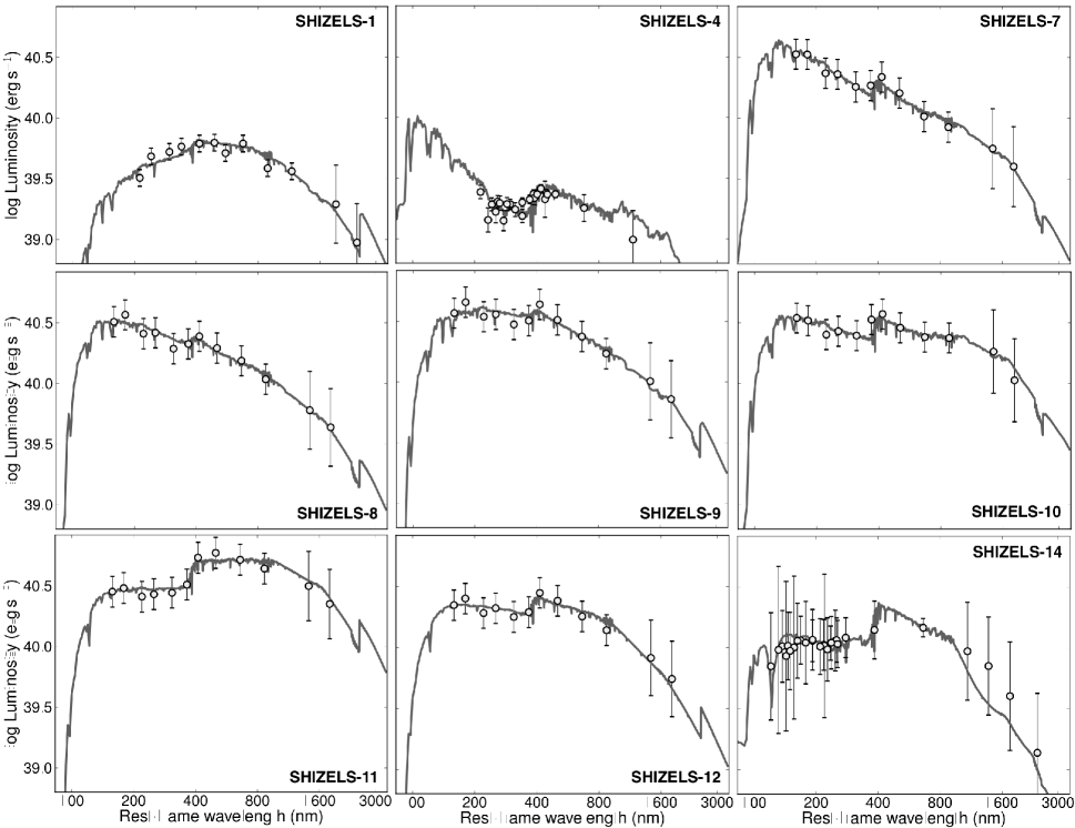
Figure 1: Broad-band photometry and SEDs for the nine galaxies in our sample from rest-frame- UV to mid-infrared bands (spanning GALEX far-UV and near-UV bands to Spitzer/IRAC). In all cases, we calculate the rest-frame spectral energy distribution (SED) and star-formation history and use this information to estimate the stellar masses (Table 2). The SEDs are calculated using a $\chi^{2}$ fit using the Bruzual & Charlot (2003) population synthesis models with a Chabrier IMF. The SHiZELS galaxies sample a range of stellar masses from $\sim$10^9-11 M_⊙ and specific star-formation rates 0.1–10 Gyr^-1.

Table 1: Targets & Observations

ID	RA	Dec	$z_{\rm H\alpha}$	$t_{\rm exp}$	Strehl	EE
	(J2000)	(J2000)		$(\rm ks)$		(0.1′′)
SHiZELS-1	02 18 26.3	$-$04 47 01.6	0.8425	9.8	15%	11%
SHiZELS-4	10 01 55.3	$+$02 14 02.6	0.8317	3.6	10%	8%
SHiZELS-7	02 17 00.4	$-$05 01 50.8	1.4550	13.4	27%	25%
SHiZELS-8	02 18 21.0	$-$05 19 07.8	1.4608	9.8	21%	27%
SHiZELS-9	02 17 13.0	$-$04 54 40.7	1.4625	9.8	24%	27%
SHiZELS-10	02 17 39.0	$-$04 44 43.1	1.4471	9.8	20%	25%
SHiZELS-11	02 18 21.2	$-$05 02 48.9	1.4858	3.6	13%	32%
SHiZELS-12	02 19 01.4	$-$04 58 14.6	1.4676	9.8	20%	30%
SHiZELS-14	10 00 51.6	+02:33 34.5	2.2418	12.0	12%	26%

Table 1: Notes: EE denotes the encircled energy within a radius of 0.1^′′.

Table 2: Integrated Galaxy Properties

ID	fHα	SFRHα	$r_{1/2}$	[Nii] / H$\alpha$	MB	MK	$\log_{\rm 10}$(M∗)	E (B $-$ V)	$\Delta$ log(O / H) / $\Delta$ R)
	($\times$10-16	(M⊙/yr)	(kpc)		(AB)	(AB)	(M⊙)		(dex kpc-1)
	erg s-1 cm-2)
SHiZELS-1	1.0 $\pm$ 0.1	2	1.8 $\pm$ 0.3	0.2 $\pm$ 0.05	$-$18.70	$-$21.54	10.03 $\pm$ 0.15	0.4 $\pm$ 0.1	$-$0.037${}_{-0.058}^{+0.030}$
SHiZELS-4	0.7 $\pm$ 0.1	1	1.4 $\pm$ 0.5	0.2 $\pm$ 0.1	$-$20.68	$-$21.49	9.74 $\pm$ 0.12	0.0 $\pm$ 0.2	…
SHiZELS-7	1.2 $\pm$ 0.1	8	3.7 $\pm$ 0.2	0.43 $\pm$ 0.05	$-$21.12	$-$22.15	9.81 $\pm$ 0.28	0.2 $\pm$ 0.2	$-$0.019${}_{-0.040}^{+0.019}$
SHiZELS-8	1.1 $\pm$ 0.1	7	3.1 $\pm$ 0.3	$<$ 0.1	$-$21.26	$-$21.90	10.32 $\pm$ 0.28	0.2 $\pm$ 0.2	+0.006${}_{-0.004}^{+0.017}$
SHiZELS-9	1.0 $\pm$ 0.1	6	4.1 $\pm$ 0.2	0.27 $\pm$ 0.03	$-$21.77	$-$22.49	10.08 $\pm$ 0.28	0.2 $\pm$ 0.2	$-$0.027${}_{-0.018}^{+0.010}$
SHiZELS-10	1.6 $\pm$ 0.2	10	2.3 $\pm$ 0.2	0.13 $\pm$ 0.04	$-$21.15	$-$21.81	9.42 $\pm$ 0.33	0.3 $\pm$ 0.2	$-$0.031${}_{-0.014}^{+0.016}$
SHiZELS-11	1.3 $\pm$ 0.1	8	1.3 $\pm$ 0.4	0.6 $\pm$ 0.1	$-$22.13	$-$24.44	11.01 $\pm$ 0.24	0.5 $\pm$ 0.2	$-$0.0870${}_{-0.006}^{+0.032}$
SHiZELS-12	0.7 $\pm$ 0.1	5	0.9 $\pm$ 0.5	0.27 $\pm$ 0.03	$-$21.34	$-$22.44	10.59 $\pm$ 0.30	0.3 $\pm$ 0.2	…
SHiZELS-14	1.6 $\pm$ 0.1	27	4.6 $\pm$ 0.4	0.60 $\pm$ 0.05	$-$23.55	$-$24.75	10.90 $\pm$ 0.20	0.4 $\pm$ 0.1	$-$0.024${}_{-0.012}^{+0.012}$
Median	1.1 $\pm$ 0.1	7 $\pm$ 2	2.4 $\pm$ 0.7	0.27 $\pm$ 0.08	$-$21.3 $\pm$ 0.20	$-$22.2 $\pm$ 0.3	10.25 $\pm$ 0.50	0.3 $\pm$ 0.1	$-$0.026 $\pm$ 0.006

Table 2: Notes: H$\alpha$ fluxes are in units of 10^-16 erg s^-1 cm^-2. The errors on the fluxes are dominated by $\sim$10% systematic uncertainties in the flux calibration from the change in Strehl ratio between observing standard stars on-axis and the target galaxies off axis. r_1/2 is the H$\alpha$ half light radius and has been deconvolved for the PSF. Errors on M_B & M_K are typically 0.15 dex (Sobral et al., 2011).

2 Sample Selection, Observations & Data Reduction

2.1 HiZELS

To select the targets for IFU observations, we exploited the high density of sources in the HiZELS imaging of the COSMOS and UDS fields (Sobral et al., 2012b) to select H$\alpha$ emitters which are close to bright (R $<$ 15.0) stars, such that natural guide star adaptive optics correction could be applied to achieve high spatial resolution. For this program, we selected fourteen galaxies with H$\alpha$ fluxes from the HiZELS catalog with fluxes between 0.7–1.6 $\times$ 10^-16 erg s^-1 cm^-2 to ensure that their star-formation properties and dynamics could be mapped in a few hours. However, of the fourteen galaxies in our parent sample, only nine systems yield a H$\alpha$ detection in the data-cubes, which may (in part) be due to spurious detections in the early HiZELS catalogs. At the three redshift ranges of our sample, the average H$\alpha$ fluxes of our galaxies correspond to star-formation rates (adopting the the Kennicutt 1998 calibration with a Chabrier IMF) of SFR = 4.6 $\times$ 10^-44 L_Hα = 1.7, 6.9 and 19.3 M_⊙ yr^-1 at $z$ = 0.83, 1.47 and 2.23 respectively.

Next we estimate the far-infrared luminosities for the galaxies in our sample. We exploit the Herschel/SPIRE imaging of these fields which were taken as part of the Herschel Multi-tiered Extra-galactic Survey (HerMES). The SPIRE maps reach 3 $\sigma$ limits of $\sim$8, 10 and 11 mJy at 250, 350 and 500$\mu$m respectively. None of the SINFONI-HiZELS (SHiZELS) galaxies in our sample are individually detected (which is unsurprising given the implied star-formation rates from H$\alpha$), but we can search for an average star-formation rate via stacking.

In the following analysis, we restrict ourselves to the $z$ = 1.47 galaxies only to mitigate against redshift effects in the stack on the SED. The 250, 350 & 500$\mu$m stacked fluxes for the $z$ = 1.47 SHiZELS galaxies of 6.9 $\pm$ 1.7, 9.0 $\pm$ 1.9 and 7.0 $\pm$ 2.4 mJy at 250, 350 and 500$\mu$m respectively (or 7.5 $\pm$ 1.6, 9.2 $\pm$ 2.2 & 7.4 $\pm$ 3.0 mJy at 250, 350 & 500$\mu$m if we instead stack all nine SHiZELS galaxies in our sample). A simple modified black-body fit to this photometry (with a dust emmisivity of $\beta$ = 1.5–2.0) at the known redshift yields a far-infrared luminosity (integrated between 8–1000$\mu$m) of L_FIR = 1.8 $\pm$ 0.6 $\times$ 10¹¹ L_⊙ and hence a total star-formation rate of SFR_FIR = 2.7 $\times$ 10^-44 L_FIR = 18 $\pm$ 8 M_⊙ yr^-1.

We note that if we instead stack all 317 HiZELS H$\alpha$ emitters from the $z$ = 1.47 parent sample with fluxes $>$1 $\times$ 10^-16 erg s^-1 cm^-2 in the UDS and COSMOS fields then the 250, 350 & 500$\mu$m fluxes are 6.3 $\pm$ 0.24, 7.9 $\pm$ 0.25 and 5.6 $\pm$ 0.31 mJy respectively, suggesting L_FIR = 1.5 $\times$ 10¹¹ L_⊙ which is consistent with our SHiZELS sample.

Next, for all of the SHiZELS galaxies, we use the broad-band imaging of the galaxies in order to calculate the rest-frame spectral energy distribution (SED), reddening and star-formation histories and stellar masses (Sobral et al., 2010). We exploit deep archival multi-wavelength imaging from rest-frame UV to mid-infrared bands (see Sobral et al. 2010 for references) and follow Sobral et al. (2011) to perform a full SED $\chi^{2}$ fit using the Bruzual & Charlot (2003) and Bruzual (2007) population synthesis models which include the Thermally Pulsating Asymptotic Giant Branch (TP-AGB) stellar phase and a Chabrier IMF (see Sobral et al. 2010 for the range of parameters). We use photometry from up to 36 (COSMOS) and 16 (UDS) wide, medium and narrow bands (spanning GALEX far-UV and near-UV bands to Spitzer/IRAC; Fig 1) and in Table 2 we give the best-fit stellar mass and E(B$-$V) for each galaxy.

The average E(B$-$V) for our sample is E(B$-$V) = 0.3 $\pm$ 0.1 which corresponds to A_Hα = 0.91 $\pm$ 0.21 (A_v = 1.11 $\pm$ 0.27). Applying this correction to the H$\alpha$ luminosities suggests reddening corrected star-formation rates SFR_Hα = 16 $\pm$ 5 M_⊙ yr^-1, which is similar to those derived from the far-infrared (SFR_FIR = 18 $\pm$ 8 M_⊙ yr^-1).

The rest-frame $B$-band magnitudes (uncorrected for extinction) and stellar masses are given in Table 2 (the 1$\sigma$ errors are drawn from the multidimensional $\chi^{2}$ distribution and are typically 0.15 dex). So that more direct comparisons can be made with other datasets, we also report the rest-frame $B$- and $K$-band magnitudes for each of the galaxies in our sample, and we note that the average inferred light-to-mass ratio is L_K/M = 0.58 $\pm$ 0.14.

Thus, overall, these galaxies appear to have luminosities consistent with local LIRGs, with dust corrections of A${}_{\rm V}\mathrel{\raise 1.50696pt\hbox{$\scriptstyle>$}\kern-6.00006pt\lower 1.72218pt\hbox{{$\scriptstyle\sim$}}}1$ and star-formation rates characteristic of “typical” star-forming galaxies at these epochs (Sobral et al., 2012b). Moreover, the SHiZELS galaxies sample a range of stellar masses from $\sim$10^9-11 M_⊙ and specific star-formation rates 0.1–10 Gyr^-1. Since one of the main high-redshift comparison samples we use throughout this paper is the SINFONI Near-Infrared Galaxy Survey (SINS; Förster Schreiber et al. 2009), we note that our sample has a comparable range of stellar masses, although the SINS sample tend to have higher H$\alpha$-derived star-formation rates, (SFR_Hα = 7 $\pm$ 2 M_⊙ yr^-1 and 30 $\pm$ 3 M_⊙ yr^-1 for SHiZELS and SINS respectively).

2.2 SINFONI Observations

To map the nebular H$\alpha$ emission line properties of the galaxies in our sample, we used the SINFONI IFU on the ESO VLT (Eisenhauer et al., 2003). The SINFONI IFU uses an image slicer and mirrors to reformat a field of 3 $\times$ 3^′′ at a spatial resolution of 0.1^′′/pixel. At $z$ = 0.84, 1.47 and 2.23 the H$\alpha$ emission line is redshifted to $\sim$ 1.21, 1.61 and 2.12$\mu$m and into the $J$, $H$ and $K$-bands respectively. The spectral resolution in each band is $\lambda$ / $\Delta\lambda\sim$ 4500 (the sky lines have 4-Å FWHM). In the remainder of our analysis, emission line widths are deconvolved for the instrumental resolution. Since each of the targets were selected to be close to a bright AO star, we used NGS correction. The $R$-band magnitude of the AO stars are $R$ = 12.0–15.0 and they have separations between 8^′′ and 40^′′ from the target galaxies.

To observe the targets we used ABBA chop sequences, nodding 1.5^′′ across the IFU. We observed each target for between 3.6 and 13.4 ks (each individual exposure was 600 seconds) between 2009 September 10 and 2011 April 30 in $\sim$0.6^′′ seeing and photometric conditions. The median Strehl achieved for our observations is 20% (Table 1) and the median encircled energy within 0.1^′′ is 25% (the approximate spatial resolution is 0.1^′′ FWHM or 850 pc at $z$ = 1.47 – the median redshift of our survey). Individual exposures were reduced using the SINFONI esorex data reduction pipeline which extracts, flat-fields, wavelength calibrates and forms the data-cube for each exposure. The final data-cube was generated by aligning the individual data-cubes and then combined these using an average with a 3-$\sigma$ clip to reject cosmic rays. For flux calibration, standard stars were observed each night either immediately before or after the science exposures. These were reduced in an identical manner to the science observations.

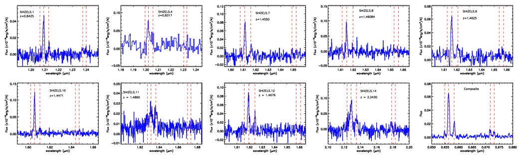
Figure 2: Spatially integrated, one dimensional spectra around the redshifted H$\alpha$ emission for each of the galaxies in our sample. In each case, the dashed lines identify the H$\alpha$, [Nii]$\lambda\lambda$ 6583,6548 and [Sii]$\lambda\lambda$ 6716,6731 emission lines. In the final panel we show the flux weighted composite spectrum. In all cases, we clearly detect [Nii] emission and the median [Nii] / H$\alpha$ for the sample is 0.3 $\pm$ 0.1, with a range of 0.1 $<$ [Nii] / H$\alpha<$ 0.6. None of the galaxies display strong AGN signatures in their near-infrared spectra (e.g. broad lines or strong [Nii] / H$\alpha$ ratios).

2.3 Galaxy Dynamics

All nine galaxies display strong H$\alpha$ emission, with a range of H$\alpha$ luminosities of L${}_{\rm H\alpha}\sim$ 10^41.4-42.4 erg s^-1. In Figure 2 we show the galaxy-integrated one-dimensional spectrum from each galaxy. In all cases we clearly detect the [Nii]$\lambda$ 6583 emission, the median [Nii] / H$\alpha$ for the sample is 0.3 $\pm$ 0.1, with a range of 0.1 $<$ [Nii] / H$\alpha$$<$ 0.6. None of the galaxies display strong AGN signatures in their near-infrared spectra.

To search for fainter lines we also transform each of the spectra to the rest-frame and coadd them (weighted by flux) and show this stack in Fig. 2. In this composite, the [Nii] / H$\alpha$ = 0.29 $\pm$ 0.02, is consistent with the average of individual measurements. We also make a clear detection of the [Sii]$\lambda\lambda$ 6716,6761 doublet and derive a flux ratio of I₆₇₁₆ / I₆₇₃₁ = 1.36 $\pm$ 0.08 which corresponds to an electron density in the range 100–1000 cm^-3 (Osterbrock, 1989) and a mass in the ISM of 3–30 $\times$ 10¹⁰ M_⊙ for a half-light radius of 2 kpc (Table 2). It is also useful to note that the [Sii] $\lambda$6716 / H$\alpha$ reflects the ionisation strength of the ISM and we derive [Sii] $\lambda$6716 / H$\alpha$ = 0.13 $\pm$ 0.04 which suggests an ionisation parameter $\log$(U / cm³) = $-$3.5 $\pm$ 0.3 (Osterbrock, 1989; Collins & Rand, 2001). This is comparable to an ionisation rate of $\log_{10}$(U / cm³) $\sim$ $-$3.9 which can be inferred from the average star-formation rate volume density of our galaxies and assuming there are 3 $\times$ 10⁶⁰ ionising photons per solar mass of star-formation (Cox, 1983).

To measure the velocity structure in each galaxy, we fit the H$\alpha$ and [Nii]$\lambda\lambda$6548,6583 emission lines pixel-by-pixel. We use a $\chi^{2}$ minimisation procedure, taking into account the greater noise at the positions of the sky lines. We first attempt to identify a line in each 0.1 $\times$ 0.1^′′ pixel ($\sim$ 1 $\times$ 1 kpc, which corresponds to the approximate PSF), and if the fit fails to detect the emission line, the region is increased to 2 $\times$ 2 pixels. Using a continuum fit we required a signal-to-noise $>$5 to detect the emission line in each pixel, and when this criterion is met we fit the H$\alpha$ and [Nii]$\lambda\lambda$ 6548,6583 emission allowing the centroid, intensity and width of the Gaussian profile to vary (the FWHM of the H$\alpha$ and [Nii] lines are coupled in the fit). Uncertainties on each parameter of the fit are calculated by perturbing one parameter at a time, allowing the remaining parameters to find their optimum values, until $\Delta\chi^{2}$ = 1 is reached.

Even with $\sim$kpc-scale resolution, we note that there is a contribution to the line widths of each pixel from the large-scale velocity motions across the PSF which must be corrected for (Davies et al., 2011). To account for this ”beam smearing”, at each pixel where the H$\alpha$ emission is detected, we calculate the local velocity gradient ($\Delta$ V  $\Delta$ R) and subtract this in quadrature from the measured velocity dispersion.

In Fig. 3 we show the H$\alpha$ intensity, velocity and line of sight velocity dispersion maps for the galaxies in our sample. There is clearly a variety of H$\alpha$ morphologies, ranging from compact (e.g. SHiZELS 11 & 12) to very extended/clumpy (e.g. SHiZELS 7, 8, 9, 14). For three galaxies, we also include high-resolution broad-band imaging thumbnails from Hubble Space Telescope ACS $V$-band (SHiZELS 4&14) or WFC3 $H$-band (SHiZELS 11) which shows that the H$\alpha$ is well correlated with the rest-frame UV/optical morphology. The distribution and intensity of star-formation (and the properties of the star-forming clumps) are discussed in a companion paper (Swinbank et al. 2012 ApJ submitted). Fig. 3 also shows that there are strong velocity gradients in many cases (e.g. SHiZELS 1, 7, 8, 9, 10, 11, & 12). We will investigate how many of these systems can be classified as “disks” in §3.

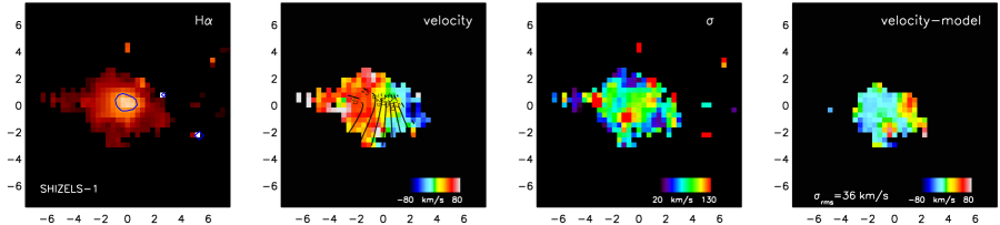
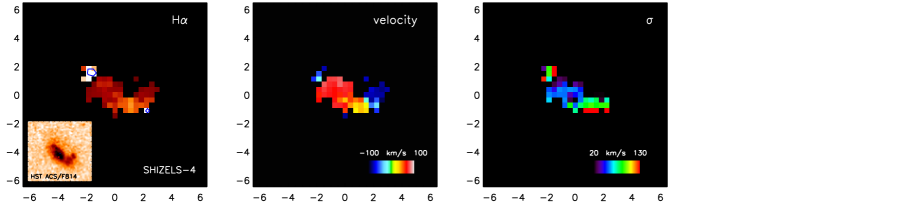
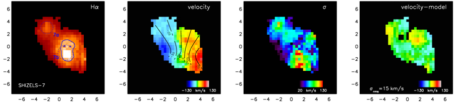
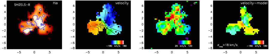
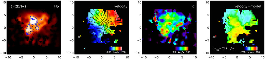
Figure 3: H$\alpha$ and kinematic maps of the SHiZELS galaxies. For each galaxy, the left hand panel shows the H$\alpha$ emission line flux. The contours denote a H$\alpha$-derived star-formation surface density of $\Sigma_{\rm SF}$ = 0.1 M_⊙ yr^-1 kpc^-2. The central two panels show the velocity field and line-of-sight velocity dispersion profile ($\sigma$) respectively. The right hand panel shows the residual velocity field after subtracting the best-fit kinematic model. The r.m.s. of these residuals is given in each panel (for SHiZELS 4 & 12 there are too few resolution elements across the source to meaningfully attempt to fit disk models).

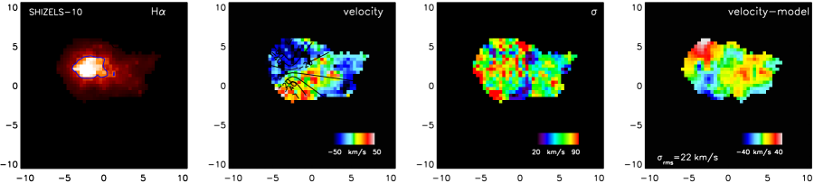
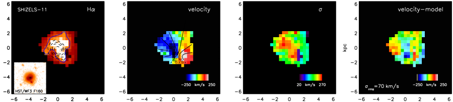
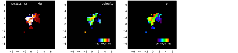
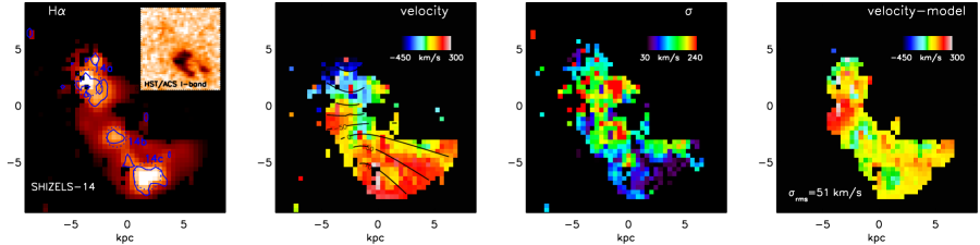
Figure 3: continued…

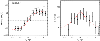
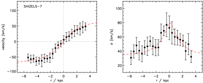
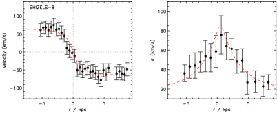
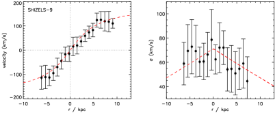
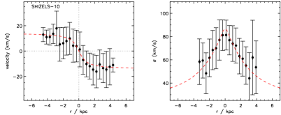
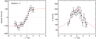
Figure 4: Left: One dimensional rotation curves for the seven galaxies in our sample which show strong velocity gradients in their H$\alpha$ dynamics. For the six galaxies whose dynamics resemble rotating systems, we overlay the best-fit one dimensional rotation curve Right: One dimensional velocity dispersion profiles with the best-fit line of sight profile overlaid for the rotating systems. The observed rotation curve and line-of-sight velocity dispersion are extracted from the two-dimensional velocity fields using a 1 kpc width slit across the major kinematic axis of each galaxy.

Table 3: Dynamical Properties

ID	vasym	$\sigma$	V2.2	Inc	KV	Kσ	KTot	$\chi^{2}_{\nu}$	Class
	(km/s)	(km/s)	(km/s)	(deg)
SHiZELS-1	112$\pm$11	98$\pm$15	86$\pm$18	40	0.12$\pm$0.17	0.17$\pm$0.81	0.20$\pm$1.03	4.8	D
SHiZELS-4	…	77$\pm$20	…	…	…	…	…	…	C
SHiZELS-7	145$\pm$10	75$\pm$11	112$\pm$15	33	0.10$\pm$0.08	0.35$\pm$0.18	0.36$\pm$0.34	3.1	D
SHiZELS-8	160$\pm$12	69$\pm$10	144$\pm$17	25	0.20$\pm$0.15	0.30$\pm$0.25	0.36$\pm$0.40	3.0	D
SHiZELS-9	190$\pm$20	62$\pm$11	155$\pm$24	54	0.12$\pm$0.05	0.48$\pm$0.20	0.49$\pm$0.30	5.7	D
SHiZELS-10	30$\pm$12	64$\pm$8	26$\pm$12	30	0.13$\pm$0.05	0.83$\pm$0.14	0.84$\pm$0.35	25.5	M
SHiZELS-11	224$\pm$15	190$\pm$18	208$\pm$18	25	0.16$\pm$0.05	0.34$\pm$0.10	0.37$\pm$0.16	5.34	D
SHiZELS-12	…	115$\pm$10	…	…	…	…	…	…	C
SHiZELS-14	…	131$\pm$17	190$\pm$25	58	0.15$\pm$0.09	0.38$\pm$0.23	0.40$\pm$0.34	9.1	M
Median	147$\pm$31	75$\pm$19	133$\pm$30	…	0.13$\pm$0.01	0.37$\pm$0.07	0.38$\pm$0.04	5.3$\pm$3.0	…

Table 3: Notes: v_asym and V_2.2 are inclination corrected. $\sigma$ is the avergae velocity dispersion across the galaxy image (and the velocity dispersion map has been corrected for ”beam smearing” effects due to the PSF, see § refsec:dynamics. The classes in the final column denote Disk (D), Merger (M) and Compact (C) (see §3)

3 Analysis, Results & Discussion

All nine galaxies display velocity gradients in their H$\alpha$ kinematics, with peak-to-peak velocity gradients ranging from 40–400 km s^-1 and a ratio of peak-to-peak difference ($v_{\rm max}$), to line of sight velocity dispersion ($\sigma$) of $v_{\rm max}$ / $\sigma$ = 0.3–2.9. Although a ratio of $v_{\rm max}$ / $\sigma$ = 0.4 has traditionally been used to crudely differentiate rotating systems from mergers (Förster Schreiber et al., 2009), more detailed kinematic modelling is essential to reliably differentiate rotating systems from mergers (Shapiro et al., 2008). We therefore begin by modelling each velocity field with a rotating disk in order to estimate the disk inclination and true rotational velocity (we exclude SHiZELS 4 & 12 from this analysis as their velocity fields are only marginally resolved by our data).

Although there have been several functional forms to describe rotation curves (such as the “multi-parameter fit”; e.g. Courteau 1997 or the “universal rotation curve; Persic et al. 1996), the simplest model which provides a good fit to most rotation curves on $\sim$ kpc scales is the arctan fit of the form $v(r)$ = $\frac{2}{\pi}$ $v_{\rm asym}$ ${\rm arctan}(r/r_{t})$, where $v_{\rm asym}$ is the asymptotic rotational velocity and r_t is the effective radius at which the rotation curve turns over (Courteau, 1997). To fit the two-dimensional velocity fields of the galaxies in our sample, we construct a two-dimensional kinematic model with six free parameters (v_asym, r_t, [x/y] centre, position angle (PA) and disk inclination) and use a genetic algorithm (Charbonneau, 1995) to find the best model. During the fitting, we limit the parameters ranges to those allowed by the data (e.g. the [x/y] center and turn over radius, r_t, must be within the SINFONI field of view; the maximum circular velocity must be $<$ 2 $\times$ the maximum velocity seen in the data; PA = 0–180^∘, and $i$ = 0–90). We then generate 10⁵ models within random initial parameters between these ranges and find the lowest $\chi^{2}_{\nu}$. This process is repeated (up to 100 times), but in each new generation we remove (up to) 10% of the worst fits and contract the remaining parameter space search by up to 5% centered on the best-fit. We examine whether the fit has converged by examining whether all of the models in a generation are within $\Delta\chi^{2}$ = 1 of the best-fit model. The errors on the final parameters (Table 3) reflect the range of acceptable models from all of the models attempted.

The best-fit kinematic maps and velocity residuals are shown in Fig. 3, whilst the best-fit inclinations and disk rotation speeds are given in Table 2, along with the $\chi^{2}_{\nu}$. All galaxies show small-scale deviations from the best-fit model, as indicated by the typical r.m.s, $<$ data $-$ model $>$ = 30 $\pm$ 10 km s^-1, with a range from $<$ data $-$ model $>$ = 15–70 km s^-1. These offsets could be caused by the effects of gravitational instability, or simply due to the unrelexed dynamical state indicated by the high velocity dispersions ($\sigma$ = 96 $\pm$ 24 km s^-1). The goodness of fit and small scale deviations from the best-fit models are similar to those of 18 galaxies in the SINS survey which show the most prominent rotational support (r.m.s of 10–80 km s^-1 and $\chi^{2}_{\nu}$ = 0.2–20; Cresci et al. 2009), as well as to the high-resolution studies of gravitationally lensed galaxies from Jones et al. (2010b) and Stark et al. (2008) (which have an average $\chi^{2}_{\nu}$ = 3.5 $\pm$ 0.8). We therefore conclude that the disk model provides an adequate fit to the majority of these galaxies and that the velocity fields of most galaxies are consistent with the kinematics of turbulent rotating disks.

We use the best-fit dynamical model to identify the major kinematic axis, and extract the one dimensional rotation curve and velocity dispersion profiles, and show these in Fig. 4. We define the zero point in the velocity using the dynamical center of the galaxy, whilst the error bars for the velocities are derived from the formal $1\sigma$ uncertainty in the velocity arising from the Gaussian profile fits to the H$\alpha$ emission. We note that in the one-dimensional rotation curves in Fig. 4 alternate points show independent data. We also note that the data have not been folded about the zero velocity, so that the degree of symmetry can be assessed.

Whilst this modelling provides a useful test of whether the dynamics can be described by disk-like rotation, a better criterion for distinguishing between motion from disturbed kinematics is the “kinemetry” which measures the asymmetry of the velocity field and line-of-sight velocity dispersion maps for each galaxy. This technique has been well calibrated and tested at low redshift (e.g.  Krajnović et al., 2006), whilst at high redshift it has been used to determine the strength of deviations of the observed velocity and dispersion maps from an ideal rotating disk (Shapiro et al., 2008). In this modelling, the velocity and velocity dispersion maps are described by a series of concentric ellipses of increasing semi-major axis length, as defined by the system center, position angle and inclination. Along each ellipse, the moment map as a function of angle is extracted and decomposed into its Fourier series which have coefficients $k_{n}$ at each radii (see Krajnović et al. 2006 for more details).

In a noiseless, idealised disk, the coefficients of the Fourier expansion would be zero. Any deviations from the ideal case that occur in a disturbed disk (e.g. warps, spiral structures, streaming motions or mergers in the extreme cases) induce strong variations in the higher-order Fourier coefficients. To ensure that reliable measurements of the kinemetry parameters can be made, we first construct a grid of 2000 model disks and mergers with noise and spatial resolution appropriate for our SINFONI observations. For the model disks, we allow disk scale lengths and rotation curve turn over lengths (r_t) from 0.5–3 kpc, rotation speeds and peak velocity dispersions from 10–300 km s^-1 and random inclinations and sky position angles. The model mergers typically comprise 2–3 of these galaxy-scale components separated by 1–20 kpc in projection. The dynamics of each of these components randomly ranges from dispersion dominated to rotating systems.

We then use the kinemetry code from Krajnović et al. (2006) and measure the velocity and velocity dispersion asymmetry for all of these models. Following Shapiro et al. (2008), we define the velocity asymmetry (K_V) as the average of the $k_{n}$ coefficients with $n$ = 2–5, normalised to the first Cosine term in the Fourier series (which represents circular motion); and the velocity dispersion asymmetry (K_σ) as the average of the first five coefficients ($n$ = 1–5) also normalised to the first Cosine term. For an ideal disk, K_v and K_σ will be zero. In a merging system, strong deviations from the idealised case causes large K_v and K_σ values, which can reach K${}_{\rm v}\sim$ K${}_{\sigma}\sim$ 10 for very disturbed systems. The total asymmetry, K_Tot is $K_{\rm Tot}^{2}$ = K${}_{\rm V}^{2}$ + K${}_{\sigma}^{2}$. For our mock sample of model disks, we recover K_Tot,disk = 0.30 $\pm$ 0.03 compared to K_Tot,merger = 2 $\pm$ 1 for the mergers.

For the SHiZELS galaxies in our sample, we measure the velocity and velocity dispersion asymmetry, (SHiZELS 4 & 12 have too few independent spatial resolution elements across the galaxy so we omit these from the kinemetry analysis). Krajnović et al. (2006) show that an incorrect choice of centre induces artificial power in the derived kinemetry coefficients. We therefore allow the dynamical center to vary over the range allowed by the family of best-fit two dimensional models and measure the kinemetry in each case. We also perturb the velocity and dispersion maps by the errors on each pixel and re-measure the asymmetry, reporting the velocity and dispersion asymmetries, (K_V and K_σ respectively) along with their errors in Table 3. We use the total asymmetry, K_Tot to differentiate disks (K${}_{\rm Tot}<$ 0.5) from mergers K${}_{\rm Tot}>$ 0.5). For the galaxies in our sample, five have are classified as disks (D), whilst two more indicate mergers (M), and the final two are compact (C).

As expected, the two galaxies that are classified as mergers from the kinemetry (SHiZELS 10 & 14) have the highest $\chi^{2}_{\nu}$ ($\chi^{2}_{\nu}>$ 9) from the dynamical modelling. Both of these systems are noteworthy; the one-dimensional rotation curve of SHiZELS 10 (extracted from the major kinematic axis) appears regular and suggests rotation, but the two-dimensional velocity field reveals extended ($\sim$ 5 kpc) emission to the east, which may be due to a companion or tidal material. The dynamics of the other galaxy classified as a merger, SHiZELS 14, are clearly more complex. The H$\alpha$ is extended across $\sim$ 14kpc with a peak-to-peak velocity gradient of $\sim$480 $\pm$ 40 km s^-1. Qualitatively, the one- and two-dimensional velocity field of SHiZELS 14 are consistent with an early stage prograde encounter, with each component in the merger displaying approximately equal peak-to-peak velocity gradients. The northern most component is also more highly obscured than the southern component (as evident from the HST $I$-band imaging; Fig. 3).

Overall, the fraction of rotating systems within our sample, $\sim$ 55%, is consistent with that found from other H$\alpha$ IFU surveys of high-redshift star-forming galaxies (e.g.  Förster Schreiber et al., 2009; Jones et al., 2010b; Wisnioski et al., 2011).

3.1 The Tully-Fisher Relation

Since our two dimensional dynamical data resolve the turn over in the rotation curves (as evident from Fig. 4), we can use our results to investigate how the disk scaling relations for the galaxies in our sample compare to galaxy disks at $z$ = 0. The relation between the rest-frame $B$-band luminosity (M_B) and rotational velocity and that between the total stellar-mass (M_⋆) and rotational velocity define the Tully-Fisher relations (Tully & Fisher, 1977). The first of these relations has a strong contribution from the short-term star-formation activity whilst the second provides a better proxy for the integrated star-formation history. Indeed the latter relationship may reflect how rotationally-supported galaxies formed, perhaps suggesting the presence of self-regulating processes for star-formation in galactic disks. The slope, intercept and scatter of the Tully-Fisher relations and their evolution are therefore key parameters that any successful galaxy formation model must reproduce (e.g.  Cole & Kaiser, 1989; Cole et al., 1994; Kauffmann et al., 1993; Eisenstein & Loeb, 1996; Somerville & Primack, 1999; Steinmetz & Navarro, 1999; Portinari & Sommer-Larsen, 2007; Dutton et al., 2011).

Since we wish to compare our dynamical measurements with those of other high-redshift galaxies where similar data exist, it is important to measure the rotational velocity in a consistent manner. Whilst the arctan function is useful for describing the overall shape of the rotation curve (in both one and two-dimensional data), it provides an extrapolation of the rotational velocity, which may not be warranted especially if the rotation curve does not flatten in the data. Equally, since any measurement of the observed peak-to-peak rotational velocity (V_max) is sensitive to the radius at which it has been possible to detect the dynamics, this measurement varies from both object-to-object depending on both the extent of the galaxy and signal-to-noise of the observations and can therefore give biased measurements when comparing samples.

A more robust measurement is that of the velocity at 2.2 times the disk scale length (V_2.2). This has a better physical basis since it measures the peak rotational velocity for a pure exponential disk (Freeman, 1970; Courteau & Rix, 1997) and provides the closest match the radio (21 cm) line widths for local galaxies (Courteau, 1997). Of course, the light profile of high-redshift galaxies are unlikely to follow pure exponential disk profiles, but it provides a reasonable estimate of where the rotation curve flattens, and as we will see below, is a good approximation of both V_max and V_asym in our data. To measure V_2.2 in our data, we therefore measure the H$\alpha$ intensity as a function of radius in our galaxies (centered at the dynamical center and using the inclination and position angle set by the best fit two-dimensional kinematic model) and infer the disk scale length (which ranges from 0.7–2.7 kpc and has a median of 1.8 $\pm$ 0.7 kpc). We then measure the rotational velocity at 2.2 disk scale lengths and report these in Table 3. The errors on these quantities are derived from both the errors on the observed velocity at this radius and the formal errors on the two-dimensional model velocity fields. For reference, we note that owing to the high resolution and signal-to-noise of our data, we have been able to resolve the flattening in the rotation curves, the ratio of the maximum (observed) peak-to-peak velocity (V_max) to V_2.2 in our sample is V_max / V_2.2 = 0.93 $\pm$ 0.05 whilst the ratio of asymptotic velocity (V_asym) to V_2.2 is V_asym / V_2.2 = 1.25 $\pm$ 0.08.

3.1.1 B-Band Tully-Fisher Relation

In Fig. 5 we show the $z$ = 0 Tully-Fisher relation from Tully & Fisher (1977) and overlay the $z$ = 0.84–2.23 measurements from our sample (using V_2.2 as the preferred measured of rotational velocity). We also include the field sample ($<z>$ = 0.33) from Bamford et al. (2005), the $z\sim$ 1 field samples from Miller et al. (2011) and Weiner et al. (2006), the $z$ = 1–3 lensed samples from Swinbank et al. (2006) and Jones et al. (2010b) and the $z\sim$ 2 and $z\sim$ 3 star-forming galaxies from Förster Schreiber et al. (2009) and Gnerucci et al. (2011) respectively.

It is clear from Fig. 5 that the $z$ = 0 $B$-band Tully-Fisher relation provides a poor fit to high-redshift data, with most of the high-redshift galaxies lying above the local relation. Since the high-redshift sample represents a heterogeneous mix of populations, all with different and complex selection functions, we limit our search for the evolution in the Tully-Fisher to its zero-point only. We therefore fix the slope to the $z$ = 0 relation and in each of the seven redshift bins from $z$ = 0.0–3 we derive the zero-point offset using a non-linear least squares regression (weighted by the velocity errors in each galaxy) and show these results in Fig. 5.

For a fixed slope, the strongest evolution occurs between $z$ = 0–1, and in this range the zero-point evolution follows $\Delta M_{\rm B}(mag)$ = ($-$1.9 $\pm$ 0.3) $z$ up to $z\sim$ 1 and then significantly flattens above $z$ = 1 to $\Delta$M${}_{\rm B}(mag)$ = ($-$0.06 $\pm$ 0.25) $z-$(1.68 $\pm$ 0.25) up to $z\sim$ 3. Since the rest-frame $B$-band is dominated by recent star-formation activity, the strong evolution in the rest-frame $B$-band Tully-Fisher zero-point between $z$ = 0 and $z$ = 1 (2 magnitudes or a factor $\sim$ 6 in luminosity) and then flattening to $z\sim$3, is consistent with the evolution of the star-formation volume density with redshift (Hopkins & Beacom, 2006).

We can compare this evolution to galaxy formation models, and in Fig. 5 we also overlay the predicted zero-point offset from the semi-analytic models from Dutton et al. (2011) and Bower et al. (2006). The Dutton et al. (2011) semi-analytic models suggest that for a fixed circular velocity, the luminosity of a galaxy at $z\sim$ 1 should be a factor up to $\sim$ 2.5 $\times$ higher than today (Dutton et al., 2011), although the data are suggestive of markedly stronger evolution than predicted by the models $z\sim$ 1. In contrast the predictions from the Bower et al. (2006) model predicts very little evolution in the $B$-band Tully-Fisher relation ($\Delta M_{B}<$ 0.2 magnitudes between $z$ = 0–4). In this model, the apparent lack of evolution in the $B$-band Tully-Fisher relation in the galaxy formation models occurs because the specific star-formation rate evolves rapidly with both mass and redshift. Although the model approximately matches the evolution of the star-formation rate density with redshift, this is offset by an increase in the specific star-formation rate in low mass galaxies. Moreover, since the dark halos are more concentrated at high-redshift, a fixed v_circ does not select the same mass halo at the two epochs (for a fixed v_circ, a halo at $z$ = 0 is a factor $\sim$1.7$\times$ more massive than at $z$ = 2). This combination of the evolution of the specific star-formation rate with mass and redshift, and the evolution in the halo densities for a fixed v_circ approximately cancel to predict that there should be very little evolution in the $B$-band Tully-Fisher relation.

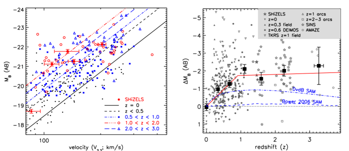
Figure 5: Left: The evolution of the rest-frame $B$-band Tully-Fisher relation. We baseline our results against the $z$ = 0 measurements from Pierce & Tully (1992). For the high-redshift samples, we combine the observations from this work with a number of other surveys. At $z\sim$ 0.1–1 we include the field surveys from Bamford et al. (2005) ($z$ = 0.3 field), Weiner et al. (2006) (TKRS $z$ = 1 field) and Miller et al. (2011) ($z$ = 0.6 DEIMOS). At $z\mathrel{\raise 1.50696pt\hbox{$\scriptstyle>$}\kern-6.00006pt\lower 1.72218pt\hbox{{$\scriptstyle\sim$}}}$ 1 we include the cluster arc surveys of Swinbank et al. (2006) ($z$ = 1 arcs) and Jones et al. (2010b) ($z$ = 2–3 arcs) and at $z\mathrel{\raise 1.50696pt\hbox{$\scriptstyle>$}\kern-6.00006pt\lower 1.72218pt\hbox{{$\scriptstyle\sim$}}}$2 we include the SINS and AMAZE surveys Förster Schreiber et al. (2009); Gnerucci et al. (2011). The solid line denotes the $z$ = 0 $B$-band Tully-Fisher relation from (Pierce & Tully, 1992). Right: The evolution of the zero-point of the $B$-band Tully-Fisher relation. The open symbols denote individual galaxies and the solid points show the median (and error) in seven redshift bins between $z$ = 0 and $z$ = 3. The curves shows the predictions of the evolution of the $B$-band Tully-Fisher relation from semi-analytic models by Bower et al. (2006) and Dutton et al. (2011) which both predict evolution of $\Delta M_{B}<$ 1 mags between $z$ = 0 and $z$ = 3, less than seen in the observations.

3.1.2 The Stellar Mass Tully-Fisher Relation

The rest-frame $B$-band Tully-Fisher relation is sensitive to recent star formation, and so perhaps the more fundamental relation is the stellar mass Tully-Fisher relation (M_⋆ versus v_asym) which reflects the time-integrated star-formation history. The $z$ = 0 stellar mass Tully-Fisher relation is well established (Bell & de Jong, 2001; Pizagno et al., 2007; Meyer et al., 2008), and in Fig. 6 we combine the stellar mass estimates with the inclination-corrected rotation speed of our galaxies to investigate how this varies as a function of redshift. Again, in this plot, we also include a number of high-redshift measurements; at $z\sim$ 0.6 and $z\sim$ 1.3 from Miller et al. (2011) and (Miller et al., 2012), the $z$ = 1–3 lensed galaxy surveys (Swinbank et al., 2006; Jones et al., 2010b; Richard et al., 2011) as well as the the $z\sim$ 2 SINS and $z>$ 3 SINFONI IFU surveys (Cresci et al., 2009; Gnerucci et al., 2011). Where necessary, we have corrected the samples to use V_2.2 using V_2.2/V_max = 0.93 if only V_max is given in the literature (see also Dutton et al. (2007)).

In comparison to the rest-frame $B$-band Tully-Fisher relation, Fig. 6 shows that the the redshift evolution in the stellar mass Tully-Fisher relation is weak. Due to the heterogeneous selection functions of these various surveys, we again restrict the search to the evolution in the zero-point with redshift. We therefore construct the same seven redshift bins from $z$ = 0–3 as in § 3.1.1 and measure the zero-point offset in each bin (using a non-linear least squares regression weighted by the velocity errors in each galaxy; (Fig. 6). The data suggest that the zero-point offset from $z$ = 2.5 to $z$ = 0 is $\Delta$M_∗,z=0 / M_⋆ = 2.0 $\pm$ 0.4 (i.e. at a fixed circular velocity the stellar mass of galaxies has increased by a factor $\sim$ 2.0 between $z$ = 2.5 and $z$ = 0). The weak evolution in the stellar mass Tully-Fisher relation (in particular below $z\sim$ 1) is due to the fact that individual galaxies evolve roughly along the scaling relation rather than due to weak evolution in the galaxies themselves (e.g.  Portinari & Sommer-Larsen, 2007; Brooks et al., 2011). This indicates that the baryon conversion efficiency, $\eta$ = (M_⋆ / M₂₀₀) / ($\Omega_{\rm b}$ / $\Omega_{\rm 0}$, is fixed with redshift.

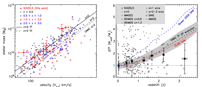
Figure 6: Left: The evolution of the stellar mass Tully-Fisher relation. We baseline the evolution against the $z$ = 0 work from Pizagno et al. (2005). The high-redshift points are compiled from the intermediate- and high- redshift ($z\sim$0.6 DEIMOS and $z\sim$1.3 DEIMOS) observations from Miller et al. (2011) and Miller et al. (2012); the $z$ = 1 and $z$ = 2–3 cluster arc surveys from Swinbank et al. (2006) and Jones et al. (2010b) with stellar masses from Richard et al. (2011); and the $z\sim$2–3.5 SINS and AMAZE surveys from Cresci et al. (2009) and Gnerucci et al. (2011). The symbols show individual galaxies. The solid line denotes the correlation at $z$ = 0 from Pizagno et al. (2005) (corrected to a Chabrier IMF). The dashed line is best-fitting zero point to the $z$ = 2 sample galaxies (for a fixed $v_{2.2}$) which shows an offset of of $\Delta$M_⋆,z=0 / M_⋆ = 2.0 $\pm$ 0.4 between $z$ = 0 and $z$ = 2.5. The dotted lines denote the Tully-Fisher at $z$ = 2 from the numerical simulations from Crain et al. (2009) and (see also McCarthy et al., 2012), which predict evolution in both the zero-point and slope. Here, we concentrate on the zero-point evolution, and note that the predicted evolution for a disk with circular velocity 100–200 km s^-1 is an increase in stellar mass of a factor 1.5–3 $\times$ between $z$ = 2 and $z$ = 0 (equivalently, at high-redshift the maximum circular velocity is greater for the same stellar mass which may be consistent with the galaxies being compact at high-redshift and larger at low-redshift). Right: The evolution of the zero-point of the Tully-Fisher Relation. The symbols denote individual points (coded by the survey), whilst the solid symbols denote the average in six redshift bins. We also overlay the redshift evolution of the zero-point of the Tully-Fisher relation from the numerical model from Crain et al. (2009) as well as the semi-analytic models from Bower et al. (2006) and Dutton et al. (2011) (DvdB). These galaxy formation models predict evolution in the zero-point of the Tully-Fisher relation out to $z\sim$ 3 which is consistent with the observed trend given the large uncertainties in the latter.

In Fig. 6 we also compare the zero-point evolution in the Tully-Fisher relation to that from semi-analytic models from Bower et al. (2006) and Dutton et al. (2011) and the cosmological hydrodynamic Galaxies–Intergalactic Medium Interaction Calculation (GIMIC, Crain et al. 2009). The Bower et al. (2006) and GIMIC simulations both use the same underlying dark matter distribution, although the GIMIC simulation follows the hydrodynamical evolution of gas, radiative cooling, star formation and chemo-dynamics, and includes a prescription for energetic feedback from supernovae. In contrast to simulations of small periodic volumes, GIMICs unique initial conditions enable it to follow, at high-resolution, cosmologically representative volumes to $z$ = 0 (see Crain et al., 2009; McCarthy et al., 2012). To search for evolution in the Tully-Fisher zero-point in the simulations, we only consider galaxies with star-formation rates $>$1 M_⊙ yr^-1 (at all redshifts) so that a reasonable comparison to observational data can be made. Both the semi-analytic and hydrodynamic simulations shown in Fig. 6 predict strong evolution, with the GIMIC simulation suggesting that, at a fixed circular velocity the stellar mass of galaxies should increase by 2.5 $\pm$ 0.5 $\times$ between $z$ = 2 and $z$ = 0. This evolution is matched by the semi-analytic model from Dutton et al. (2011). However, the semi-analytic model from Bower et al. (2006) predicts somewhat stronger evolution in the stellar mass for a fixed circular velocity.

It is interesting to note that the GIMIC simulation predicts that the scatter in the Tully-Fisher relation should not evolve strongly with redshift (for a fixed circular velocity, the scatter is 25 $\pm$ 5% over the redshift range $z$ = 0–3). Our dynamical measurements, particularly when combined with those from Weiner et al. (2006) and Miller et al. (2012), are sufficiently large in number to compare to the models, and Fig. 6 shows that the scatter in the observations is consistent with the models (for all but the last bin in redshift where the number of data-points is $<$8), , suggesting that the samples may now be sufficiently large (with rotation curves well enough sampled) that the scatter is intrinsic.

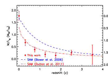
Figure 7: The $B$-band mass-to-light ratio as a function of redshift for star-forming galaxies from this work plus the compilation of studies shown in Fig. 5 and  6. The dashed- and dot-dashed- lines show the predicted evolution of the mass-to-light ratio as a function of redshift from the Bower et al. (2006) and Dutton et al. (2011) semi-analytic models. This figure shows that in both the observations and galaxy formation models there is strong evolution in the mass-to-light ratio of galaxies with redshift. The strongest evolution in the data is seen for $z$ = 0–1, with significant flattening above $z$ = 1.

3.2 The Redshift Evolution of the Mass-to-Light ratio

Another route to examine the evolution in the $B$-band and stellar mass Tully-Fisher relations is to combine the offsets and measure the evolution of the mean mass-to-light ratio with redshift. We caution that the conversion of zero-point offsets to offsets in mass-to-light assumes that star-forming galaxies form a homologous family and that the evolution is a manifestation of underlying relations between mass-to-light ratio and other parameters, such as star-formation history, gas accretion and stellar feedback.

Under these assumptions, in Fig. 7 we show the evolution of the rest-frame $B$-band mass-to-light ratio. As expected from the zero-point Tully-Fisher offsets, this figure shows that the average mass to light ratio of star-forming galaxies decreases strongly from $z$ = 0 up to $z$ = 1 and then flattens. This behavior is consistent with the previous demonstration that star-forming galaxies at high-redshift have lower stellar masses and higher $B$-band luminosities. The strongest evolution occurs up to $z\sim$ 1, $\Delta$M_⋆ / L_B = 1.1 $\pm$ 0.2, consistent with previous studies (Miller et al., 2011) (the fractional change in mass-to-light ratio over this period is $\Delta$(M / L_B) / (M / L_B)${}_{\rm z=0}\sim$ 3.5 between $z$ = 1.5 and $z$ = 0, with most of the evolution occuring below $z$ = 1).

We note that we examined whether the evolution in the mass-to-light ratio could be reproduced using simple star-formation histories, ranging from i) a constant star-formation rate (with a formation redshift, $z_{f}$ = 4–8); or ii) a set of exponentially decreasing star-formation rates with $e$-folding times ranging from 0.25–10 Gyr (and formation redshifts ranging from $z_{f}$ = 2–10). However, using these simple star-formation histories (adopting a Chabrier IMF with 0.5–1 solar metallicities and the Padova (1994) stellar evolution tracks), we are unable to find a acceptable fit with a single star-formation history. This could be because the ”average” star-formation history is more complex than a simple star-formation model, or because the current low and high-redshift data can not be linked by a simple evolutionary model. However, in Fig. 7 we also overlay the predicted evolution of the $B$-band mass-to-light ratio from the semi-analytic models of Bower et al. (2006) and Dutton et al. (2011), both of which predict a sharp decline to $z\sim$ 1 and then flattening to higher redshift, which provides a reasonable match to the observations.

3.3 The Evolution of the Size–Rotational Velocity Relation

In a $\Lambda$CDM cosmology, the sizes of galaxy disks and their rotational velocities should be proportional to their parent dark halos, and since the halos are denser at higher redshift, for fixed circular velocity the disk sizes should scale inversely with Hubble time (Mo et al., 1998). In this scenario, disks at $z$ = 1 and $z$ = 2 should be 1.8 and 3.0 $\times$ smaller respectively at fixed circular velocity. With the high-resolution measurements for the galaxies in our sample we can measure the extent of the H$\alpha$ (and together with the dynamics) compare these relations at $z\sim$ 1.5 to star-forming disks at $z$ = 0.

In Fig. 8 we show the relation between the H$\alpha$ half-light radius and rotational velocity for the galaxies in our sample (using the asymptotic velocity as measured from the disk modeling). In this plot, we also include the measurements from the SINS galaxies from Cresci et al. (2009). First, we note that the H$\alpha$ half-light radii for the SHiZELS galaxies ($r_{h}$ = 2.4 $\pm$ 0.8 kpc) are comparable to the average rest-frame UV/optical half light radii of star-forming galaxies at this redshift (e.g. Conselice et al., 2003; Law et al., 2007; Swinbank et al., 2010).

In order to compare to $z$ = 0 data, we show the measurements of local disks from Navarro & Steinmetz (2000) (which is based on a compilation from Mathewson et al. 1992 and Courteau 1997), but converting the disk scale length (r_d) to half-light radius using r_1/2 = 1.68 r_d, as appropriate for a disk with an exponential profile. As can be seen from this figure, the high-redshift galaxies have half-light sizes (deconvolved for seeing) which are smaller for fixed circular velocity than those at $z$ = 0. Fitting the local the $z$ = 0 relation to the high-redshift data (only allowing a zero-point shift and inverse weighting the fit by the errors on each data-point) suggests that this offset is a factor $\Delta r_{\rm h}$ / r_h,z=0 = 1.4 $\pm$ 0.3, which is consistent (given the smaller number statistics in the high-redshift measurements) with that predicted from halo–disk scaling arguments (Mo et al. 1998; see also Dutton et al. 2011).

The product of the rotational velocity and size of the disk define the specific angular momentum, and the evolution (at a fixed circular velocity) with redshift also encodes information on the relation between the star-formation processes in the disk and the halo spin parameters (e.g.  Navarro & Steinmetz, 2000; Tonini et al., 2006). The offsets seen in the r_1/2–v_asym relation compared to local scaling relations in Fig. 8 translate directly into offsets in the specific angular momentum for disks between $z$ = 0 and $z\sim$ 2. Indeed, the offsets in r_1/2–v_asym suggest that, for fixed circular velocity the specific angular momentum of disks at $z$ = 2 is a factor 1.4 $\pm$ 0.3 lower than those at $z$ = 0 (Navarro & Steinmetz, 2000). Thus, if high-redshift disks evolve into local disk galaxies, then the specific angular momentum must be increased, either by removing material with low specific angular momentum through outflows, or the galaxy disk must decouple from the halo and acquire angular momentum from accreting gas.

Finally, in Fig. 8 we also show the relation between stellar mass and H$\alpha$ half light radius for the galaxies in our sample compared to the $z$ = 0 relation from Dutton et al. (2007). The high-redshift galaxies are offset from the local relation by $\Delta r_{\rm rh}$ / r_h = 1.2 $\pm$ 0.3 for a fixed stellar mass. Although this is consistent with no evolution, we note that the predicted evolution for a fixed stellar mass between $z$ = 0–2 from the semi-analytic model from Dutton et al. (2011) is $\Delta r_{\rm rh}$ / r_h = 1.2.

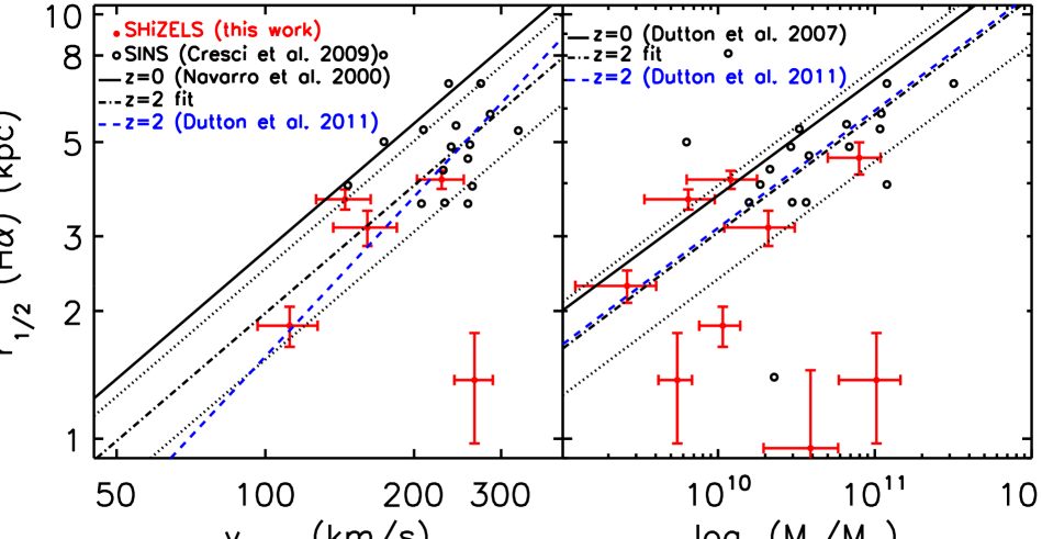
Figure 8: Left: The relation between the circular-velocity and H$\alpha$ half-light radius for high-redshift galaxies. We include the results from the SHiZELS galaxies in our sample as well as those from SINS (Cresci et al., 2009). The solid line shows the $z$ = 0 relation from Navarro & Steinmetz (2000) (which is based on a compilation from Mathewson et al. 1992 and Courteau 1997). Fitting the local relation (assuming a fixed slope) to the high-redshift points suggests and offset $\Delta r_{\rm h}$ / r_h,z=0 = 1.4 $\pm$ 0.3, which is shown by the dot-dashed line (the scatter is shown by the dotted lines). This evolution is consistent with that predicted by halo–disk scaling arguments (e.g. Dutton et al. 2011; blue dashed line). Right: the relation between stellar-mass and half-light radius in the SHiZELS and SINS surveys. The solid line shows the $z$ = 0 relation from Dutton et al. (2011) whilst the dot-dashed curve shows the offset of the high-redshift measurements from the local relation (assuming a fixed slope), which shows a $\Delta r_{\rm rh}$ / r_h = 1.2 $\pm$ 0.3 offset for a fixed stellar mass. We also show the predicted evolution of $z$ = 2 galaxies from the $z$ = 0 relation from the Dutton et al. (2011) semi-analytic model.

3.4 Metallicities and Spatially Resolved Chemical Abundances

The internal enrichment (and radial abundance gradients) of high-redshift star-forming galaxies provides a tool for studying the gas accretion and mass assembly process such as gas exchange (inflows/outflows) with the intergalactic medium. However, the small sizes of high redshift galaxies (typically r${}_{\rm h}\sim$ 2–3 kpc; e.g. Law et al. 2007; Conselice et al. 2008; Smail et al. 2007; Swinbank et al. 2010) mean that sub-kpc resolution observations are required to measure the abundances reliably. At high redshifts the gas-phase metallicity of individual galaxies can only be measured with limited accuracy, usually through the [Nii] / H$\alpha$ emission-line ratio as an indicator of oxygen abundance and calibrations between gas phase emission line and stellar absorption metallicities, such as those obtained by Pettini & Pagel (2004). Recently, the first reliable spatially resolved measurements of [Nii] / H$\alpha$ have been made in two highly amplified galaxies at $z\sim$ 1.5–2.5, measuring strong, negative gradients and suggesting that if $z\sim$ 2 starbursts evolve into spiral disks today, then the gradients must flatten by $\Delta$ log(O / H) / $\Delta$R$\sim$ 0.05–0.1 dex kpc over the last 8–10 Gyr (Jones et al., 2010a; Yuan et al., 2011). Other studies at lower resolution have derived weaker gradients that are negative, or consistent with zero for rotating and interacting galaxies (Cresci et al., 2010; Queyrel et al., 2012). Positive gradients for interacting systems may be a signature of the redistribution of the metal-rich gas produced from a central starburst; (Werk et al., 2010; Rupke et al., 2010), or possibly as a result of inflow of relatively unenriched gas from the halo (or IGM) if it is able to intersect the central regions of the disk galaxy without being disrupted.

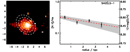
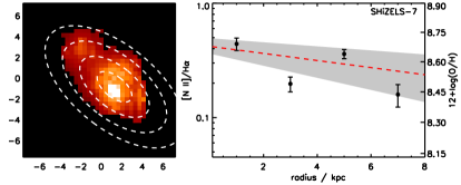
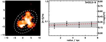
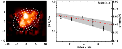
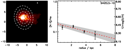
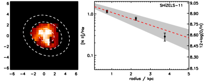
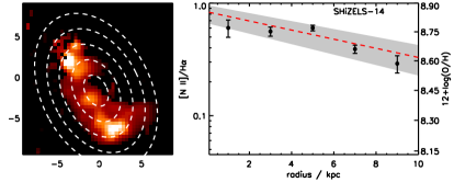
Figure 9: Metallicity gradients for the seven galaxies in our sample where spatially resolved measurements can be made. Left: Velocity integrated H$\alpha$ emission line maps. The dashed annuli denote the $\sim$ 1 kpc regions from which the [Nii]/H$\alpha$ were extracted. Right: The [Nii]$\lambda$ 6583 / H$\alpha$ emission line ratio as a function of physical radius. We overlay the best-fit linear regression and we report the gradients for individual galaxies in Table 1. In all cases the gradients are negative or consistent with zero, as expected for inside-out growth.

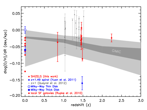
Figure 10: Metallicity gradients versus redshift for the galaxies in our sample compared to the Milky-Way and other low- and high-redshift observations. The Milky-Way thin and thick disk measurements are from Gilmore et al. (1995); Bell (1996); Robin et al. (1996); Edvardsson et al. (1993); the low-redshift star-forming galaxies are from Rupke et al. (2010) and the $z$ = 1–1.5 data from Yuan et al. (2011) and Queyrel et al. (2012). The median abundance gradient for our SHiZELS sample is $\Delta$ log(O / H) / $\Delta$R = $-$0.027 $\pm$ 0.005 dex kpc^-1 which is consistent with the thick disk of the Milky-Way. We also show the theoretical evolution of the metallicity gradient with redshift from the GIMIC simulation (Crain et al., 2009; McCarthy et al., 2012). The dark grey shows the range of metallicity gradients for all disk galaxies in the simulation in the mass range 9.5 $<$ log(M / M_⊙) $<$ 11.5, whilst the light grey denotes the 1$\sigma$ scatter at each epoch. The GIMIC simulation predicts the gradients should be steep around $z\sim$ 3 where gas accretion from the IGM is at its most efficient, but should flatten by a factor $\sim$2 $\times$ between $z$ = 3 and $z$ = 0.

With our high-resolution (and high signal-to-noise) resolved observations we can measure the spatially resolved emission line ratios and hence the distribution of chemical abundances. First, we note that the average galaxy integrated [Nii] / H$\alpha$  ratio for the galaxies in our sample is [Nii] / H$\alpha$  = 0.27 $\pm$ 0.09, which corresponds to 12 + log(O / H) = 8.58 $\pm$ 0.07 (equivalently, $\sim$ 0.73 $\pm$ 0.16 Z_⊙ where Z_⊙ is 12 + log(O / H) = 8.66 $\pm$ 0.05; Asplund et al. 2004). We caution that the [Nii]/H$\alpha$ ratio is sensitive to shock excitation, the ionization state of the gas, and the hard ionization radiation field from an active galactic nucleus (Kewley & Dopita, 2002; Kewley et al., 2006; Rich et al., 2010). However, our galaxy-integrated [Nii] / H$\alpha$ ratios are consistent with star formation throughout the disk (Fig. 2).

Of the nine galaxies in our high-redshift sample, seven have [Nii]$\lambda$6583 emission which is sufficiently strong (S/N$>$10 in the combined spectra) to allow spatially resolved studies of the chemical abundance gradients. First we subtract the large-scale velocity motions from the data-cube (as defined by the best-fit dynamical model). We then use the disk inclination and position angle to define $\sim$1 kpc annuli (centered at the dynamical center) and integrate the spectrum in each annulus to measure the [Nii] / H$\alpha$ ratio. In Fig. 9 we show the H$\alpha$ emission line maps as well as the spatially resolved [Nii] / H$\alpha$ ratio and overlay the best-fit linear regression in each case. We report the gradients individually in Table 2. In all cases, the metallicity gradients are negative or consistent with zero, with an average $\Delta$ log(O / H) / $\Delta$R = $-$0.027 $\pm$ 0.005 dex kpc^-1, and similar to those recently found for a sample of $z\sim$ 1 starbursts (Queyrel et al., 2012). This average gradient is steeper, but consistent with the thick disk of the Milky-Way, $\Delta$ log(O / H) / $\Delta$R = $-$0.01 $\pm$ 0.02 dex kpc^-1 (Gilmore et al., 1995; Bell, 1996; Robin et al., 1996; Edvardsson et al., 1993), which has a mass weighted age of 8–12 Gyr (equivalently, a formation redshift $z$ = 2–4; Bensby et al. 2007; Ruchti et al. 2011).

In Fig. 10 we compare the metallicity gradients to those from the GIMIC simulation (which include cold gas accretion from the IGM). We calculate the disc phase metallicity in cylindrical coordinates (along the disc) at $z$ = 0, 1, 2 & 3 in radial bins of width 1 kpc for all galaxies in the simulation with masses between M_⋆ = 10^9.5-11 M_⊙. At $z\sim$ 2, the model disk galaxies from the GIMIC simulation display negative metallicity gradients which are consistent with our observations. Moreover, between $z$ = 2 and $z$ = 0 the GIMIC simulation predicts that the gradient should flatten by a factor $\sim$ 2. In the simulation, this is a consequence of the outer disk enrichment increasing with decreasing redshift (as the gas inflow rates decline and gas is redistributed) progressively flattening the radial gradient within the thick disk. This is qualitatively similar to the numerical models of Dekel et al. (2009a) and where the “cold streams” (which are most prevalent around $z\sim$2) penetrate the halo and intersect and deposit relatively unenriched gas at onto the galaxy disks at $\sim$15 kpc (Dekel et al., 2009a, b).

4 Conclusions

We have presented AO-assisted, spatially resolved spectroscopy of nine star-forming galaxies at $z$ = 0.84–2.23 selected from the UKIRT, wide-field narrow-band, HiZELS survey (Sobral et al., 2012b). Our main results can be summarised as:

$~{}\bullet$ Using H$\alpha$ emission line dynamics, we find that the ratio of dynamical-to-dispersion support for the sample is $v_{\rm max}$ sin($i$) / $\sigma$ = 0.3–3, with a median of 1.1 $\pm$ 0.3, which is consistent with similar measurements for both AO and non-AO studies of star-forming galaxies at this epoch(e.g.  Förster Schreiber et al., 2009). At least six galaxies have dynamics that suggest that their ionised gas is in a large, rotating disk (in at least four of these we detect the turn over in their rotation curves). For these galaxies that resemble rotating systems, we model the galaxy velocity field and derive the inclination-corrected, asymptotic velocity.

$~{}\bullet$ We combine our dynamical observations with a number of previous studies of intermediate- and high-redshift galaxies (in particular from Bamford et al. 2005; Weiner et al. 2006; Förster Schreiber et al. 2009; Jones et al. 2010b; Miller et al. 2011 and Miller et al. 2012) to investigate the evolution of the Tully-Fisher relation. We show that there is strong evolution in the zero-point of the rest-frame $B$-band Tully-Fisher relations with redshift such that at a fixed circular velocity, the $B$-band luminosity increases by $\Delta$ M_B = 2 mags up to $z\sim$ 2 (a change in luminosity of a factor $\sim$ 6; e.g. see also Bamford et al. 2005; Weiner et al. 2006; Miller et al. 2011).

$~{}\bullet$ In contrast, the stellar mass Tully-Fisher relation shows much more modest evolution; for a fixed circular velocity the average stellar masses has increased by a factor 2.0$\pm$0.4 between $z$ = 2 and $z$ = 0 (e.g. see also Cresci et al. 2009; Miller et al. 2012). The weak evolution in the stellar mass Tully-Fisher relation (in particular below $z\sim$ 1) is due to the fact that individual galaxies evolve along the scaling relations rather than due to weak evolution in the galaxies themselves (e.g.  Portinari & Sommer-Larsen, 2007; Brooks et al., 2011; Dutton et al., 2011), and indicates that the baryon conversion efficiency, $\eta$ = (M_∗ / M₂₀₀) / ($\Omega_{\rm b}$ / $\Omega_{\rm 0}$), is fixed with redshift. The observations also suggest that the scatter in high-redshift Tully-Fisher relation is comparable to that predicted by the models, suggesting that the samples may now be sufficiently large (with rotation curves well enough sampled) that the scatter is intrinsic.

$~{}\bullet$ Combining the rest-frame $B$-band and stellar mass Tully-Fisher relations we show that the mass-to-light ratio of star-forming galaxies evolves strong with redshift, decreasing by $\Delta$ M / L_B = 1.1 $\pm$ 0.2 between $z$ = 0 and $z$ = 1, but then ceases to evolve further above $z$ = 1. This change in mass-to-light ratio in the $B$-band is a factor $\Delta$ (M / L_B) / (M / L_B)${}_{\rm z=0}\sim$ 3.5. We show that the evolution in the Tully-Fisher relations and mass-to-light ratio is in line with both cosmologically-based hydrodynamic simulations and semi-analytic models of galaxy formation.

$~{}\bullet$ Using the H$\alpha$ half light radius and circular velocity, we also find that the SHiZELS galaxies are a factor 1.5 $\pm$ 0.3 $\times$ smaller for fixed circular velocity than for disks at $z$ = 0. If the $z\sim$ 2 and $z$ = 0 disks are linked in a simple evolutionary scenario then high-redshift disks must acquire specific angular momentum, either by removing material with low specific angular momentum (e.g. through outflows), or through acquisition of angular momentum from accreted gas at late times.

$~{}\bullet$ Finally, we measure the spatially resolved [Nii] / H$\alpha$ to measure the metallicity gradients. In all cases, the metallicity gradients are negative or consistent with zero, with an average $\Delta$ log(O / H) / $\Delta$ R = $-$0.027 $\pm$ 0.005 dex kpc^-1, which is consistent with that seen in the thick disk of the Milky-Way. We show that these metallicity gradients are comparable to those predicted for the gas disks of star-forming galaxies in the cosmologically based hydrodynamic simulations. In these models, the inner disk undergoes initial rapid collapse and star-formation with gas accretion (either from the halo and/or IGM) depositing relatively unenriched material at the outer disk, causing negative abundance gradients. At lower redshift (when gas accretion from the IGM is less efficient) the abundance gradients flatten as the outer disk becomes enriched by star-formation (and/or the redistribution of gas from the inner disk).

Overall, we demonstrate that well-sampled, dynamical measurements of high-redshift star-forming galaxies can constrain the rotation curves, measure the evolution of the basic disk scaling relations and their radial abundance gradients. We show that the current observational samples with well resolved data are now approaching sufficiently large samples that it is possible to refine or refute models of disk galaxy formation.

References

- Asplund et al. (2004) Asplund, M., Grevesse, N., Sauval, A. J., Allende Prieto, C., & Kiselman, D. 2004, A&A, 417, 751
- Bamford et al. (2005) Bamford, S. P., Milvang-Jensen, B., Aragón-Salamanca, A., & Simard, L. 2005, MNRAS, 361, 109
- Bell (1996) Bell, D. J. 1996, PASP, 108, 1139
- Bell & de Jong (2001) Bell, E. F. & de Jong, R. S. 2001, ApJ, 550, 212
- Bensby et al. (2007) Bensby, T., Zenn, A. R., Oey, M. S., & Feltzing, S. 2007, ApJL, 663, L13
- Benson et al. (2003) Benson, A. J., Bower, R. G., Frenk, C. S., Lacey, C. G., Baugh, C. M., & Cole, S. 2003, ApJ, 599, 38
- Bournaud & Elmegreen (2009) Bournaud, F. & Elmegreen, B. G. 2009, ApJL, 694, L158
- Bower et al. (2006) Bower, R. G., Benson, A. J., Malbon, R., Helly, J. C., Frenk, C. S., Baugh, C. M., Cole, S., & Lacey, C. G. 2006, MNRAS, 370, 645
- Brooks et al. (2011) Brooks, A. M., Solomon, A. R., Governato, F., McCleary, J., MacArthur, L. A., Brook, C. B. A., Jonsson, P., Quinn, T. R., & Wadsley, J. 2011, ApJ, 728, 51
- Bruzual & Charlot (2003) Bruzual, G. & Charlot, S. 2003, MNRAS, 344, 1000
- Chabrier (2003) Chabrier, G. 2003, PASP, 115, 763
- Charbonneau (1995) Charbonneau, P. 1995, ApJS, 101, 309
- Cole et al. (1994) Cole, S., Aragon-Salamanca, A., Frenk, C. S., Navarro, J. F., & Zepf, S. E. 1994, MNRAS, 271, 781
- Cole & Kaiser (1989) Cole, S. & Kaiser, N. 1989, MNRAS, 237, 1127
- Collins & Rand (2001) Collins, J. A. & Rand, R. J. 2001, ApJ, 551, 57
- Conselice et al. (2003) Conselice, C. J., Bershady, M. A., Dickinson, M., & Papovich, C. 2003, AJ, 126, 1183
- Conselice et al. (2008) Conselice, C. J., Rajgor, S., & Myers, R. 2008, MNRAS, 386, 909
- Courteau (1997) Courteau, S. 1997, AJ, 114, 2402
- Courteau & Rix (1997) Courteau, S. & Rix, H.-W. 1997, Bulletin of the American Astronomical Society, 29, 1332
- Cox (1983) Cox, D. P. 1983, ApJL, 265, L61
- Crain et al. (2009) Crain, R. A., Theuns, T., Dalla Vecchia, C., Eke, V. R., Frenk, C. S., Jenkins, A., & Kay, S. T. 2009, MNRAS, 399, 1773
- Cresci et al. (2009) Cresci, G., Hicks, E. K. S., Genzel, R., Schreiber, N. M. F., Davies, R., Bouché, N., Buschkamp, P., & Genel, S. et al. 2009, ApJ, 697, 115
- Cresci et al. (2010) Cresci, G., Mannucci, F., Maiolino, R., Marconi, A., Gnerucci, A., & Magrini, L. 2010, Nature, 467, 811
- Daddi et al. (2010) Daddi, E., Bournaud, F., Walter, F., Dannerbauer, H., Carilli, C. L., Dickinson, M., Elbaz, D., & Morrison G. et al. 2010, ApJ, 713, 686
- Davies et al. (2011) Davies, R., Förster Schreiber, N. M., Cresci, G., Genzel, R., Bouché, N., Burkert, A., Buschkamp, P., & Genel, S. et al. 2011, ApJ, 741, 69
- Dekel et al. (2009a) Dekel, A., Birnboim, Y., Engel, G., Freundlich, J., Goerdt, T., Mumcuoglu, M., Neistein, A., & Pichon, C et al. 2009a, Nature, 457, 451
- Dekel et al. (2009b) Dekel, A., Sari, R., & Ceverino, D. 2009b, ApJ, 703, 785
- Desmond (2012) Desmond, H. 2012, ArXiv e-prints
- Dutton et al. (2007) Dutton, A. A., van den Bosch, F. C., Dekel, A., & Courteau, S. 2007, ApJ, 654, 27
- Dutton et al. (2011) Dutton, A. A., van den Bosch, F. C., Faber, S. M., Simard, L., Kassin, S. A., Koo, D. C., Bundy, K., & Huang, J. et al. 2011, MNRAS, 410, 1660
- Edvardsson et al. (1993) Edvardsson, B., Andersen, J., Gustafsson, B., Lambert, D. L., Nissen, P. E., & Tomkin, J. 1993, A&A, 275, 101
- Eisenhauer et al. (2003) Eisenhauer, F., Abuter, R., Bickert, K., Biancat-Marchet, F., Bonnet, H., Brynnel, J., Conzelmann, R. D., & Delabre, B., et al. 2003, in Instrument Design and Performance for Optical/Infrared Ground-based Telescopes. Edited by Iye, Masanori; Moorwood, Alan F. M. Proceedings of the SPIE, Volume 4841, pp. 1548-1561 (2003)., ed. M. Iye & A. F. M. Moorwood, 1548–1561
- Eisenstein & Loeb (1996) Eisenstein, D. J. & Loeb, A. 1996, ApJ, 459, 432
- Ferguson et al. (1998) Ferguson, A. M. N., Gallagher, J. S., & Wyse, R. F. G. 1998, AJ, 116, 673
- Fernández Lorenzo et al. (2009) Fernández Lorenzo, M., Cepa, J., Bongiovanni, A., Castañeda, H., Pérez García, A. M., Lara-López, M. A., Pović, M., & Sánchez-Portal, M. 2009, A&A, 496, 389
- Förster Schreiber et al. (2009) Förster Schreiber, N. M., Genzel, R., Bouché, N., Cresci, G., Davies, R., Buschkamp, P., Shapiro, K., & Tacconi, L. J.. et al. 2009, ApJ, 706, 1364
- Förster Schreiber et al. (2006) Förster Schreiber, N. M., Genzel, R., Lehnert, M. D., Bouché, N., Verma, A., Erb, D. K., Shapley, A. E., & Steidel, C et al. 2006, ApJ, 645, 1062
- Freeman (1970) Freeman, K. C. 1970, ApJ, 160, 811
- Geach et al. (2008) Geach, J. E., Smail, I., Best, P. N., Kurk, J., Casali, M., Ivison, R. J., & Coppin, K. 2008, MNRAS, 388, 1473
- Geach et al. (2011) Geach, J. E., Smail, I., Moran, S. M., MacArthur, L. A., Lagos, C. d. P., & Edge, A. C. 2011, ApJL, 730, L19
- Genzel et al. (2006) Genzel, R., Tacconi, L. J., Eisenhauer, F., Förster Schreiber, N. M., Cimatti, A., Daddi, E., Bouché, N., & Davies, R., et al. 2006, Nature, 442, 786
- Gilmore & Wyse (1985) Gilmore, G. & Wyse, R. F. G. 1985, AJ, 90, 2015
- Gilmore et al. (1995) Gilmore, G., Wyse, R. F. G., & Jones, J. B. 1995, AJ, 109, 1095
- Gnerucci et al. (2011) Gnerucci, A., Marconi, A., Cresci, G., Maiolino, R., Mannucci, F., Calura, F., Cimatti, A., & Cocchia, F. et al. 2011, A&A, 528, A88
- Hopkins & Beacom (2006) Hopkins, A. M. & Beacom, J. F. 2006, ApJ, 651, 142
- Hopkins et al. (2012) Hopkins, P. F., Quataert, E., & Murray, N. 2012, MNRAS, 421, 3488
- Jones et al. (2010a) Jones, T., Ellis, R., Jullo, E., & Richard, J. 2010a, ApJL, 725, L176
- Jones et al. (2010b) Jones, T. A., Swinbank, A. M., Ellis, R. S., Richard, J., & Stark, D. P. 2010b, MNRAS, 404, 1247
- Kauffmann et al. (1993) Kauffmann, G., White, S. D. M., & Guiderdoni, B. 1993, MNRAS, 264, 201
- Kennicutt (1998) Kennicutt, R. C. 1998, ARAA, 36, 189
- Kereš et al. (2005) Kereš, D., Katz, N., Weinberg, D. H., & Davé, R. 2005, MNRAS, 363, 2
- Kewley & Dopita (2002) Kewley, L. J. & Dopita, M. A. 2002, ApJS, 142, 35
- Kewley et al. (2006) Kewley, L. J., Groves, B., Kauffmann, G., & Heckman, T. 2006, MNRAS, 372, 961
- Krajnović et al. (2006) Krajnović, D., Cappellari, M., de Zeeuw, P. T., & Copin, Y. 2006, MNRAS, 366, 787
- Krumholz & McKee (2005) Krumholz, M. R. & McKee, C. F. 2005, ApJ, 630, 250
- Law et al. (2007) Law, D. R., Steidel, C. C., Erb, D. K., Pettini, M., Reddy, N. A., Shapley, A. E., Adelberger, K. L., & Simenc, D. J. 2007, ApJ, 656, 1
- Mathewson et al. (1992) Mathewson, D. S., Ford, V. L., & Buchhorn, M. 1992, ApJS, 81, 413
- McCall et al. (1985) McCall, M. L., Rybski, P. M., & Shields, G. A. 1985, ApJS, 57, 1
- McCarthy et al. (2012) McCarthy, I. G., Schaye, J., Font, A. S., Theuns, T., Frenk, C. S., Crain, R. A., & Dalla Vecchia, C. 2012, ArXiv e-prints
- Meyer et al. (2008) Meyer, M. J., Zwaan, M. A., Webster, R. L., Schneider, S., & Staveley-Smith, L. 2008, MNRAS, 391, 1712
- Miller et al. (2011) Miller, S. H., Bundy, K., Sullivan, M., Ellis, R. S., & Treu, T. 2011, ApJ, 741, 115
- Miller et al. (2012) Miller, S. H., Ellis, R. S., Sullivan, M., Bundy, K., Newman, A. B., & Treu, T. 2012, ApJ, 753, 74
- Mo et al. (1998) Mo, H. J., Mao, S., & White, S. D. M. 1998, MNRAS, 295, 319
- Navarro & Steinmetz (2000) Navarro, J. F. & Steinmetz, M. 2000, ApJ, 538, 477
- Osterbrock (1989) Osterbrock, D. E. 1989, Astrophysics of gaseous nebulae and active galactic nuclei
- Persic et al. (1996) Persic, M., Salucci, P., & Stel, F. 1996, MNRAS, 281, 27
- Pettini & Pagel (2004) Pettini, M. & Pagel, B. E. J. 2004, MNRAS, 348, L59
- Pierce & Tully (1992) Pierce, M. J. & Tully, R. B. 1992, ApJ, 387, 47
- Piontek & Steinmetz (2011) Piontek, F. & Steinmetz, M. 2011, MNRAS, 410, 2625
- Pizagno et al. (2005) Pizagno, J., Prada, F., Weinberg, D. H., Rix, H.-W., Harbeck, D., Grebel, E. K., Bell, E. F., & Brinkmann, J. et al. 2005, ApJ, 633, 844
- Pizagno et al. (2007) Pizagno, J., Prada, F., Weinberg, D. H., Rix, H.-W., Pogge, R. W., Grebel, E. K., Harbeck, D., & Blanton, M. et al. 2007, AJ, 134, 945
- Portinari & Sommer-Larsen (2007) Portinari, L. & Sommer-Larsen, J. 2007, MNRAS, 375, 913
- Queyrel et al. (2012) Queyrel, J., Contini, T., Kissler-Patig, M., Epinat, B., Amram, P., Garilli, B., Le Fèvre, O., Moultaka, J., Paioro, L., Tasca, L., Tresse, L., Vergani, D., López-Sanjuan, C., & Perez-Montero, E. 2012, A&A, 539, A93
- Reddy et al. (2006) Reddy, B. E., Lambert, D. L., & Allende Prieto, C. 2006, MNRAS, 367, 1329
- Rich et al. (2010) Rich, J. A., Dopita, M. A., Kewley, L. J., & Rupke, D. S. N. 2010, ApJ, 721, 505
- Richard et al. (2011) Richard, J., Jones, T., Ellis, R., Stark, D. P., Livermore, R., & Swinbank, M. 2011, MNRAS, 413, 643
- Robin et al. (1996) Robin, A. C., Haywood, M., Creze, M., Ojha, D. K., & Bienayme, O. 1996, A&A, 305, 125
- Ruchti et al. (2011) Ruchti, G. R., Fulbright, J. P., Wyse, R. F. G., Gilmore, G. F., Bienaymé, O., Bland-Hawthorn, J., Gibson, B. K., & Grebel, E. K., et al. 2011, ApJ, 737, 9
- Rupke et al. (2010) Rupke, D. S. N., Kewley, L. J., & Chien, L.-H. 2010, ApJ, 723, 1255
- Sales et al. (2010) Sales, L. V., Navarro, J. F., Schaye, J., Dalla Vecchia, C., Springel, V., & Booth, C. M. 2010, MNRAS, 409, 1541
- Savage & Sembach (1996) Savage, B. D. & Sembach, K. R. 1996, ARAA, 34, 279
- Scannapieco et al. (2011) Scannapieco, C., White, S. D. M., Springel, V., & Tissera, P. B. 2011, MNRAS, 417, 154
- Searle (1971) Searle, L. 1971, ApJ, 168, 327
- Shapiro et al. (2008) Shapiro, K. L., Genzel, R., Förster Schreiber, N. M., Tacconi, L. J., Bouché, N., Cresci, G., Davies, R., & Eisenhauer, F. et al. 2008, ApJ, 682, 231
- Shields (1974) Shields, G. A. 1974, ApJ, 193, 335
- Smail et al. (2007) Smail, I., Swinbank, A. M., Richard, J., Ebeling, H., Kneib, J.-P., Edge, A. C., Stark, D., Ellis, R. S., Dye, S., Smith, G. P., & Mullis, C. 2007, ApJL, 654, L33
- Snow & Witt (1996) Snow, T. P. & Witt, A. N. 1996, ApJL, 468, L65
- Sobral et al. (2010) Sobral, D., Best, P. N., Geach, J. E., Smail, I., Cirasuolo, M., Garn, T., Dalton, G. B., & Kurk, J. 2010, MNRAS, 404, 1551
- Sobral et al. (2009) Sobral, D., Best, P. N., Geach, J. E., Smail, I., Kurk, J., Cirasuolo, M., Casali, M., & Ivison, R. J. et al. 2009, MNRAS, 398, 75
- Sobral et al. (2012a) Sobral, D., Best, P. N., Matsuda, Y., Smail, I., Geach, J. E., & Cirasuolo, M. 2012a, MNRAS, 420, 1926
- Sobral et al. (2011) Sobral, D., Best, P. N., Smail, I., Geach, J. E., Cirasuolo, M., Garn, T., & Dalton, G. B. 2011, MNRAS, 411, 675
- Sobral et al. (2012b) Sobral, D., Smail, I., Best, P. N., Geach, J. E., Matsuda, Y., Stott, J. P., Cirasuolo, M., & Kurk, J. 2012b, ArXiv:1202.3436
- Solway et al. (2012) Solway, M., Sellwood, J. A., & Schönrich, R. 2012, MNRAS, 422, 1363
- Somerville & Primack (1999) Somerville, R. S. & Primack, J. R. 1999, MNRAS, 310, 1087
- Stark et al. (2008) Stark, D. P., Swinbank, A. M., Ellis, R. S., Dye, S., Smail, I. R., & Richard, J. 2008, Nature, 455, 775
- Steinmetz & Navarro (1999) Steinmetz, M. & Navarro, J. F. 1999, ApJ, 513, 555
- Swinbank et al. (2006) Swinbank, A. M., Bower, R. G., Smith, G. P., Smail, I., Kneib, J.-P., Ellis, R. S., Stark, D. P., & Bunker, A. J. 2006, MNRAS, 368, 1631
- Swinbank et al. (2011) Swinbank, A. M., Papadopoulos, P. P., Cox, P., Krips, M., Ivison, R. J., Smail, I., Thomson, A. P., Neri, R., Richard, J., & Ebeling, H. 2011, ApJ, 742, 11
- Swinbank et al. (2010) Swinbank, A. M., Smail, I., Chapman, S. C., Borys, C., Alexander, D. M., Blain, A. W., Conselice, C. J., Hainline, L. J., & Ivison, R. J. 2010, MNRAS, 405, 234
- Tacconi et al. (2010) Tacconi, L. J., Genzel, R., Neri, R., Cox, P., Cooper, M. C., Shapiro, K., Bolatto, A., & Bournaud, F., et al. 2010, Nature, 463, 781
- Tonini et al. (2006) Tonini, C., Lapi, A., & Salucci, P. 2006, ApJ, 649, 591
- Tonini et al. (2011) Tonini, C., Maraston, C., Ziegler, B., Böhm, A., Thomas, D., Devriendt, J., & Silk, J. 2011, MNRAS, 415, 811
- Tully & Fisher (1977) Tully, R. B. & Fisher, J. R. 1977, A&A, 54, 661
- van de Voort et al. (2012) van de Voort, F., Schaye, J., Altay, G., & Theuns, T. 2012, MNRAS, 421, 2809
- van de Voort et al. (2011) van de Voort, F., Schaye, J., Booth, C. M., Haas, M. R., & Dalla Vecchia, C. 2011, MNRAS, 414, 2458
- van Zee et al. (1998) van Zee, L., Salzer, J. J., & Haynes, M. P. 1998, ApJL, 497, L1
- Vila-Costas & Edmunds (1992) Vila-Costas, M. B. & Edmunds, M. G. 1992, MNRAS, 259, 121
- Vogt (1999) Vogt, N. P. 1999, in ASP Conf. Ser. 193: The Hy-Redshift Universe: Galaxy Formation and Evolution at High Redshift, 145
- Vogt et al. (1996) Vogt, N. P., Forbes, D. A., Phillips, A. C., Gronwall, C., Faber, S. M., Illingworth, G. D., & Koo, D. C. 1996, ApJL, 465, L15
- Weiner et al. (2006) Weiner, B. J., Willmer, C. N. A., Faber, S. M., Harker, J., Kassin, S. A., Phillips, A. C., Melbourne, J., Metevier, A. J., Vogt, N. P., & Koo, D. C. 2006, ApJ, 653, 1049
- Werk et al. (2010) Werk, J. K., Putman, M. E., Meurer, G. R., Thilker, D. A., Allen, R. J., Bland-Hawthorn, J., Kravtsov, A., & Freeman, K. 2010, ApJ, 715, 656
- Wisnioski et al. (2011) Wisnioski, E., Glazebrook, K., Blake, C., Wyder, T., Martin, C., Poole, G. B., Sharp, R., & Couch, W. et al. 2011, MNRAS, 417, 2601
- Yuan et al. (2011) Yuan, T.-T., Kewley, L. J., Swinbank, A. M., Richard, J., & Livermore, R. C. 2011, ApJL, 732, L14
- Zaritsky et al. (1994) Zaritsky, D., Kennicutt, R. C., & Huchra, J. P. 1994, ApJ, 420, 87