An iterative method for the canard explosion
in general planar systems

Abstract

The canard explosion is the change of amplitude and period of a limit cycle born in a Hopf bifurcation in a very narrow parameter interval. The phenomenon is well understood in singular perturbation problems where a small parameter controls the slow/fast dynamics. However, canard explosions are also observed in systems where no such parameter is present. Here we show how the iterative method of Roussel and Fraser, devised to construct regular slow manifolds, can be used to determine a canard point in a general planar system of nonlinear ODEs. We demonstrate the method on the van der Pol equation, showing that the asymptotics of the method is correct, and on a templator model for a self-replicating system.

1 Introduction

Since the original discovery of canards in the van der Pol equation more than 30 years ago [1], they have been identified in numerous systems of nonlinear ODEs. A canard is a trajectory which stays close to a repelling slow manifold for an extended amount of time. Canards play a key role as parts of transitional limit cycles linking small cycles born in a Hopf bifurcation with large relaxation oscillations when a parameter is varied. Since this transition typically takes place over a very short parameter interval, and easily may be mistaken for a discontinuous event, the phenomenon has been denoted a canard explosion.

The mathematical theory for canards is well-established for singular perturbation systems of the form

$$\dot{x}=f(x,y,c,\epsilon),\quad\dot{y}=\epsilon g(x,y,c,\epsilon),$$ (1)

where $\epsilon$ is a small parameter and $c$ is a bifurcation parameter see e.g. [1, 8, 10]. In particular, asymptotic expansions in terms of $\epsilon$ of the canard point $c_{c}$, the parameter values where the longest canards exist, can be obtained [13, 3]. However, canard explosions have also been observed in many systems that do not have an explicit slow/fast structure with a well-defined small parameter $\epsilon$,

$$\dot{x}=F(x,y,c),\quad\dot{y}=G(x,y,c).$$ (2)

In some cases a small parameter can be identified after coordinate transformations [4], while in other cases an artificial parameter must be introduced to allow an asymptotic expansion [5, 6]. After the expansion, the artificial parameter is set to one to recover the original system.

While these approaches have been successful, they are somewhat ad-hoc, and it would be of interest to establish a systematic approach to identify and locate canard explosions in general systems of the form Eqns. (2). The purpose of the present paper is to provide such a procedure. It is a simple modification of the iterative method by Fraser and Roussel [9, 11] for finding slow manifolds. We show that for the van der Pol equation with a distinguished small parameter the method gives the correct asymptotic result. For the templator model [4] with no small parameter we get an excellent agreement between the canard point found from simulations and the lowest-order canard point from the method.

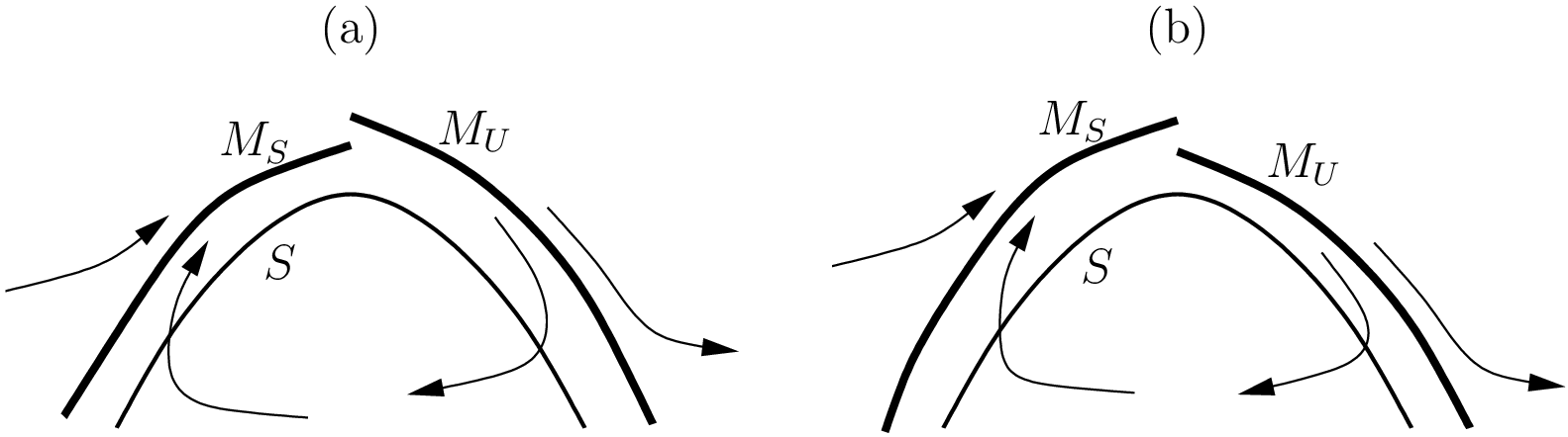
Figure 1: Canard explosion in a singular perturbation system, Eqns. (1). As trajectories cross the fold of the critical manifold $S$, they are either repelled down or up, depending on the relative position of the slow manifolds $M_{S}$ and $M_{U}$.

2 The canard explosion

Here we briefly review the basics of the theory for the canard explosion for Eqns. (1). The curve defined by $f(x,y,c,0)=0$ is denoted the critical manifold $S$. For $\epsilon=0$, $S$ consists of fixed points and assuming that it has a fold, the local phase portrait is as shown in Fig. 1. For $\epsilon>0$ it follows from standard Fenichel theory (see e.g. [12]) that on the stable side of $S$ an attracting slow manifold $M_{S}$ exists and on the unstable side a repelling slow manifold $M_{U}$ exists. The existence and the normal hyperbolicity of these manifolds is guaranteed by the theory away from the fold point only. However, as trajectories they may be extended across the fold point. In general, $M_{S}$ and $M_{U}$ will be distinct, but for a special value of $c=c_{c}$ they may coincide and form a single trajectory, a canard. Clearly, the shape of a limit cycle will change dramatically if the parameter is varied across $c_{c}$. If $M_{U}$ is above $M_{S}$ as in Fig. 1(a) only small limit cycles will be possible. If $M_{U}$ is below $M_{S}$ as in Fig. 1(b) the limit cycles will be large.

The single trajectory $M_{S}=M_{U}$ and the corresponding parameter value $c_{c}$ can be found asymptotically. For the equation for the trajectories

$$f(x,y,c,\epsilon)\frac{dy}{dx}=\epsilon g(x,y,c,\epsilon)$$ (3)

a Poincaré-Lindstedt series is inserted,

$$y=y_{0}+y_{1}\epsilon+y_{2}\epsilon^{2}+\cdots,\quad c_{c}=c_{0}+c_{1}\epsilon+c_{2}\epsilon^{2}+\cdots.$$ (4)

Collecting terms of the same order in $\epsilon$ algebraic equations for the $y_{k}$ are obtained. These will in general have a singularity at the fold point, but there will be a choice of $c_{k-1}$ such that this singularity cancels and $y_{k}$ is well-defined at the fold point. This choice defines the canard point and $y_{k}$ is the corresponding canard solution.

3 A general iterative procedure

For Eqns. (2) we can also write down the equation for the trajectories,

$$F(x,y,c)\frac{dy}{dx}=G(x,y,c).$$ (5)

Following Fraser and Roussel [9, 11], we solve this equation for $y$ algebraically,

$$y=\Phi\left(x,\frac{dy}{dx},c\right).$$ (6)

Clearly, it must be assumed that such a solution exists, at least locally. From this equation an iterative procedure can be established,

$$y_{k}=\Phi\left(x,\frac{dy_{k-1}}{dx},c\right).$$ (7)

To start the iteration we choose $y_{0}$ such that $F(x,y_{0}(x,c),c)=0$, that is, the $\infty$-isocline. Again, we must assume that this equation can be solved for $y_{0}$. Other choices will be possible, but we do not have space here to discuss this issue. Typically $y_{k}$ will have a singularity. Since $y_{k}$ depends on $c$, we will choose the value in each step such that this singularity cancels. This defines the procedure for finding canards and canard points for Eqns. (2).

4 The van der Pol equation

We now demonstrate the iterative method on the van der Pol equation

$$\dot{x}=y-(x^{3}/3-x),\quad\dot{y}=\epsilon(c-x).$$ (8)

This system has a canard explosion for $c$ close to 1 when $\epsilon$ is small and positive. The procedure from § 2 yields for the canard point [13]

$$c_{c}=1-\frac{1}{8}\epsilon-\frac{3}{32}\epsilon^{2}-\frac{173}{1024}\epsilon^{3}+{\mathcal{O}}(\epsilon^{4}).$$ (9)

The iterative procedure Eqn. (7) is defined by

$$y_{k+1}=x^{3}/3-x+\epsilon\frac{c-x}{y^{\prime}_{k}}$$ (10)

with starting point

$$y_{0}=x^{3}/3-x.$$ (11)

4.1 A numerical example

We consider first the van der Pol system Eqns. (8) with $\epsilon=0.1$. The asymptotic formula for the canard point Eqn. (9) yields $c_{c}=0.986394$.

The iterative process runs as follows: From Eqn. (10) we find

$$y_{1}=x^{3}/3-x+\frac{1}{10}\frac{c-x}{x^{2}-1}.$$ (12)

This has a singularity at $x=1$ (and also at $x=-1$, but this is not of interest here) which is removed by choosing $c=1$, which, then, is the first approximation to the canard point. The relative deviation from the asymptotic value is $1.38\%$. With this choice of $c$ we have

$$y_{1}=x^{3}/3-x-\frac{1}{10}\frac{1}{x+1}$$ (13)

and a further iteration yields

$$y_{2}=x^{3}/3-x+\frac{(x+1)^{2}(c-x)}{p_{2}}$$ (14)

where

$$p_{2}=10x^{4}+20x^{3}-20x-9.$$ (15)

The polynomial $p_{2}$ has two real roots, $x_{1}=-0.603433$ and $x_{2}=0.987258$. We remove the singularity of $y_{2}$ at the latter point by choosing $c=x_{2}=0.987258$, which is the second approximation to the canard point. This deviates from the asymptotic value by $0.09\%$.

By factorization we get

$$p_{2}=(x-x_{2})q_{2}$$ (16)

where

$$q_{2}=10x^{3}+29.8726x^{2}+29.4919x+9.11616$$ (17)

such that

$$y_{2}=x^{3}/3-x-\frac{(x+1)^{2}}{q_{2}}.$$ (18)

By iteration we find $y_{3}$, which is a rational function where the denominator is a polynomial of degree 8 in $x$ but independent of $c$. The real roots are $-1.24503$, $-0.999999$, $-0.389117$ and $x_{3}=0.986481$. The numerator of $y_{3}$ is a polynomial of degree 11 in $x$ but linear in $c$. The singularity at $x_{3}$ can be canceled by choosing $c=x_{3}=0.986481$. This gives yet an improvement of the canard point, as the deviation from the asymptotic value is now down to $0.009\%$. Clearly, the procedure can be continued any number of times.

4.2 Asymptotic analysis

The structure of the van der Pol equation is sufficiently simple to allow an asymptotic analysis in the limit $\epsilon\rightarrow 0$ of the iterative procedure. For a general $\epsilon$, we get in the first iteration

$$y_{1}=x^{3}/3-x+\frac{c-x}{x^{2}-1}\epsilon.$$ (19)

As before, we eliminate the singularity at $x=1$ by choosing $c=1$ such that

$$y_{1}=x^{3}/3-x-\frac{1}{x+1}\epsilon.$$ (20)

The next iteration gives

$$y_{2}=x^{3}/3-x+\frac{(x+1)^{2}(c-x)}{p_{2}}\epsilon$$ (21)

where

$$p_{2}=x^{4}+2x^{3}-2x-1+\epsilon.$$ (22)

The function $y_{2}$ has a singularity at $x=x_{2}$ where $x_{2}$ is a root of $p_{2}$ and the singularity cancels if $c=c_{2}=x_{2}$. The polynomial $p_{2}$ has two roots for $\epsilon<27/16$, so the construction of the canard trajectory only works under this condition. When $\epsilon=27/16$, $p_{2}$ has a double root at $x=1/2$. We choose as $x_{2}$ the root which is greater than $1/2$. By a Taylor expansion, one easily finds

$$x_{2}=c_{2}=1-\frac{1}{8}\epsilon-\frac{3}{128}\epsilon^{2}-\frac{15}{2048}\epsilon^{3}+O(\epsilon^{4}).$$ (23)

This agrees with (9) to $O(\epsilon)$, but not to $O(\epsilon^{2})$. Inserting $c=c_{2}$ from Eq. (23) in $y_{2}$ and iterating in Eq. (10) yields $y_{3}$ as a rational function. In this, we let $c=c_{0}+c_{1}\epsilon+c_{2}\epsilon^{2}+\cdots$ and in a Taylor expansion the first terms are

$$y_{3}=\frac{c_{0}-x}{(x-1)(x+1)}\epsilon+\frac{c_{1}x^{4}+2c_{1}x^{3}-(2c_{1}+1)x-c_{0}-c_{1}}{(x-1)^{2}(x+1)^{4}}\epsilon^{2}+\cdots$$ (24)

By choosing $c_{0}=1$ and $c_{1}=-1/8$ the singularities at $x=1$ in the first two terms cancel. Proceeding to the term of order $\epsilon^{3}$ (we omit the rather long expression) one cancels a singularity by choosing $c_{2}=-3/32$. Continuing this way, we find an approximation to the canard point as

$$c=1-\frac{1}{8}\epsilon-\frac{3}{32}\epsilon^{2}-\frac{75}{1024}\epsilon^{3}+O(\epsilon^{4})$$ (25)

This agrees with (9) to $O(\epsilon^{2})$, but not to $O(\epsilon^{3})$. Again, we may continue this procedure to any order, in each step correcting a term in the asymptotic expansion of the canard point.

5 The templator

The templator is a mathematical model for the kinetics of a self-replicating chemical system. The reactions are

$$X_{0}\rightarrow X$$

$$X+X\rightarrow T$$

$$X+X+T\rightarrow T+T$$

$$T\rightarrow P$$

The key process the third one where a dimer $T$ acts as a templates and catalyzes its own production from a monomer $X$. In dimensionless variables the model can be written

(a)	(b)

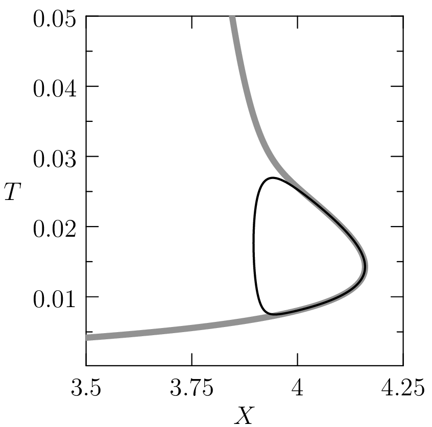
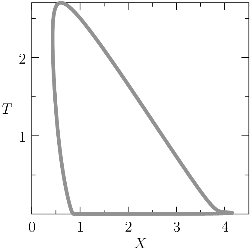
(c)

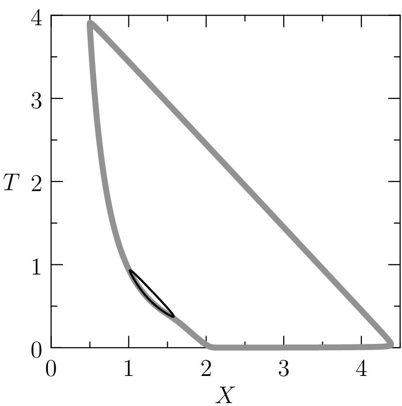
Figure 2: Simulations of the templator model Eqns. (26). (a) The black curve is the limit cycle for $r=0.419940$, the gray curve is is a part of the limit cycle for $r=0.419945$. (b) The full large limit cycle from panel (a). Note the differences in the scales. (c) The gray curve is the limit cycle for $r=0.96755$, the black curve the limit cycle for $r=0.96756$.

$$\frac{dX}{dt} =r-k_{u}X^{2}-k_{T}X^{2}T,$$ (26a)

$$\frac{dT}{dt} =k_{u}X^{2}+k_{T}X^{2}T-\frac{qT}{K+T}.$$ (26b)

The last step in the reaction is modeled as an enzymatic reaction with Michaelis-Menten kinetics. For further details on the model and its biological significance see [2, 4] and references therein.

In the following we fix the parameters $k_{u}=0.01$, $k_{T}=1$, $q=1$, $K=0.02$ and consider $r$ as a bifurcation parameter. In [2, 4] it is shown numerically that two canard explosions occur in the model. One is at $r=0.419942$ where a small limit cycle explodes as $r$ increases. The large limit cycle persists until $r=0.967555$, where it turns into a small cycle in another canard explosion. See Fig. 2. There is no obvious small parameter in the equations, so the standard asymptotic approach for Eqns. (1) does not work. However, in [4] it is shown that it is possible to account for the two canard explosions by two different scalings of the equations. Here we show that the iterative method described in this paper can be applied directly on the unscaled equations.

The equation for the trajectories is

$$\left(k_{u}X^{2}+k_{T}X^{2}T-\frac{qT}{K+T}\right)\frac{dX}{dT}=r-k_{u}X^{2}-k_{T}X^{2}T.$$ (27)

This is a quadratic equation in $X$. Choosing the positive solution, we get for the iteration process

$$X_{k+1}=\sqrt{\frac{r(K+T)+qTX_{k}^{\prime}}{(X_{k}^{\prime}+1)(k_{u}+k_{T}T)(K+T)}}.$$ (28)

To start the iteration, we choose the $dT/dt=0$ isocline as the initial approximation,

$$X_{0}=\sqrt{\frac{qT}{(k_{u}+k_{T}T)(K+T)}}.$$ (29)

The expression for $X_{1}$ which is quite complicated has a denominator which is independent of $r$. It has two zeroes, $T=0.0143454$ and $T=0.599393$. Inserting these in the numerator of $X_{1}$ and requiring that it is zero to cancel the singularity yields a linear equation to determine $r$ with solutions $r=0.417681$ and $r=0.967710$ respectively. The first canard point deviates from the numerically determined one by $0.6\%$, while the latter deviates with $0.02\%$. Hence, a very accurate determination of the canard point is achieved in the very first iteration.

6 Conclusions

We have demonstrated that a very simple iteration procedure can be used to determine canard points in general planar dynamical systems with no distinguished small parameter. We have shown for the van der Pol equation that we obtain an asymptotically correct result in the limit of $\epsilon\rightarrow 0$, and we conjecture this is a general result for problems on the classical singular perturbation form. For the more complex templator system, the method successfully found the two canard points in one iteration. In the analytical approach [4] different scalings were needed to find the two canard points.

It is interesting to note that for the van der Pol equation an upper bound for the small parameter $\epsilon$ for canard explosion to occur was found. Recently a bound of $\epsilon<1/4$ was found from consideration of the curvature of the trajectories [7]. The present bound is more conservative, and it would be interesting to obtain a clearer understanding of the relation of the two approaches to canard explosion. Furthermore, the present iterative procedure provides a new view on canard explosion which may lead to a more general understanding on the specific conditions needed for a planar dynamical system without a small parameter to experience a canard explosion. Since systems with canard explosions of this kind are abundant in the applications this seems to be of fundamental interest. Work along these lines is in progress, and will be reported elsewhere.

References

- [1] E. Benoit, J. L. Callot, F. Diener, and M. Diener. Chasse au canard. Collectanea Mathematica, 32:37–119, 1981.
- [2] K. M. Beutel and E. Peacock-López. Complex dynamics in a cross-catalytic self-replication mechanism. Journal of Chemical Physics, 126:125104, 2007.
- [3] M. Brøns. Relaxation oscillations and canards in a nonlinear model of discontinuous plastic deformation in metals at very low temperatures. Proceedings of the Royal Society of London Series A, 461:2289–2302, 2005.
- [4] M. Brøns. Canard explosion of limit cycles in templator models of self-replication mechanisms. Journal of Chemical Physics, 134:144105, 2011.
- [5] M. Brøns and K. Bar-Eli. Asymptotic analysis of canards in the EOE equations and the role of the inflection line. Proceedings of the Royal Society of London Series A, 445:305–322, 1994.
- [6] M. Brøns and J. Sturis. Explosion of limit cycles and chaotic waves in a simple nonlinear chemical system. Physical Review E, 64:026209, 2001.
- [7] M. Desroches and M. R: Jeffrey. Canards and curvature: the ’smallness’ of in slow-fast dynamics. Proceedings of the Royal Society of London Series A, 467:2404–2421, 2011.
- [8] W. Eckhaus. Relaxation oscillations includig a standard chase on french ducks. In Asymptotic Analysis II, volume 985 of Lecture Notes in Mathematics, pages 449–494. Springer Verlag, New York/Berlin, 1983.
- [9] S. J. Fraser. The steady state and equilibrium approximations: A geometrical picture. Journal of Chemical Physics, 88(8):4732–4738, 1988.
- [10] M. Krupa and P. Szmolyan. Relaxation oscillations and canard explosion. Journal of Differential Equations, 174:312–368, 2001.
- [11] M. R. Roussel and S. J. Fraser. Geometry of the steady-state approximation: Perturbation and accelerated convergence methods. Journal of Chemical Physics, 93(2):1072–1081, 1990.
- [12] F. Verhulst. Methods and Applications of Singular Perturbations. Number 50 in Texts in Applied Mathematics. Springer, New York, 2005.
- [13] A. K. Zvonkin and M. A. Shubin. Non-standard analysis and singular perturbations of ordinary differential equations. Russian Mathematical Surveys, 39(2):77–127, 1984.