Slow dynamics in cylindrically confined colloidal suspensions

Abstract

We study bidisperse colloidal suspensions confined within glass microcapillary tubes to model the glass transition in confined cylindrical geometries. We use high speed three-dimensional confocal microscopy to observe particle motions for a wide range of volume fractions and tube radii. Holding volume fraction constant, we find that particles move slower in thinner tubes. The tube walls induce a gradient in particle mobility: particles move substantially slower near the walls. This suggests that the confinement-induced glassiness may be due to an interfacial effect.

1 Introduction

Understanding the glass transition is one of the enduring questions of solid-state physics Götze and Sjögren (1992); Ediger et al. (1996); Debenedetti and Stillinger (2001); Cavagna (2009); Dyre (2006); Berthier et al. (2011). The problem is simply stated: in some cases, when a hot viscous liquid is cooled, the viscosity rises dramatically but smoothly as a function of temperature. At some temperature the viscosity is so large that the sample appears like a solid; this identifies the glass transition temperature. The same phenomenon can likewise be induced by increasing the density (increasing the pressure) Roland et al. (2005). In contrast to a regular phase transition which occurs at well-defined temperatures and pressures, the glass transition can depend on details such as the cooling rate. Likewise, while phase transitions are signaled by abrupt changes in the sample properties or their derivatives, the properties of a glass-forming material such as viscosity and diffusivity change smoothly, and to an extent the definition of the transition temperature (or pressure) is a bit arbitrary Alba-Simionesco et al. (2006); Hunter and Weeks (2012). One of the key questions is what is changing microscopically that is responsible for the macroscopic changes in viscosity; no structural length scale has yet been found that would clearly explain the viscosity change Ernst et al. (1991); Charbonneau et al. (2012).

One clever way to probe length scales is to confine a sample: rather than studying a macroscopically large sample (a “bulk” sample), studying a microscopic-scale sample. Many experiments show that glasses change their properties when their size is sufficiently small, both for small-molecule glasses and polymer glasses Roth and Dutcher (2005); Alcoutlabi and McKenna (2005); Alba-Simionesco et al. (2006); Richert (2011). One of the key observations is that the glass transition temperature $T_{g}$ changes for confined samples. In some cases $T_{g}$ increases: confined samples are glassier. However, in other cases $T_{g}$ decreases. The key difference explaining the increase or decrease seems to be the boundary conditions Richert (2011). Samples with free surfaces, such as thin free-standing polymer films, are less glassy (lower $T_{g}$). Samples confined to pores or on substrates can be more glassy (larger $T_{g}$), in particular if the sample molecules form strong chemical bonds to the confining boundaries.

We wish to use colloidal samples as a glass-forming system which can be studied in confinement. Colloidal suspensions are composed of solid particles in a liquid. As the particle concentration is increased, the sample becomes more and more viscous Marshall and Zukoski (1990); Segrè et al. (1995); Poon et al. (1996); Cheng et al. (2002). Above a critical concentration, the sample behaves as a glass, and a large number of similarities have been observed between the colloidal glass transition and glass transitions of polymers and small molecules Hunter and Weeks (2012). The most widely studied colloidal glass transition is that of hard-sphere-like colloids, and the control parameter is the volume fraction $\phi$ Pusey and van Megen (1986). The glass transition point has been identified as $\phi_{g}\approx 0.58$, with simulations demonstrating that this requires some polydispersity Zaccarelli et al. (2009); Pusey et al. (2009).

Experimentally, the colloidal glass transition shifts to lower volume fractions in confined samples: confinement makes colloidal samples glassier Nugent et al. (2007); Edmond et al. (2010, 2012); Sarangapani and Zhu (2008); Sarangapani et al. (2011); Eral et al. (2009). This has been studied exclusively in parallel-plate geometries, where samples are confined between two glass walls that are closely spaced. Often these experiments use bidisperse samples (mixtures of two particle sizes) so that the flat walls do not induce crystallization Nugent et al. (2007); Edmond et al. (2012). An alternate approach is to roughen the walls Sarangapani and Zhu (2008).

The geometry of these prior colloidal experiments most closely resembles thin films, which are used to study the glass transition of polymers or small molecule glass formers in thin slits. However, small molecule glass formers are more commonly studied by using nanoporous substrates; a variety of these nanoporous substrates are reviewed in Ref. Alba-Simionesco et al. (2006). Some of these substrates are quite disordered with pores of a variety of shapes and sizes. Others are ordered: for example, porous oxide ceramics have a regular lattice of cylindrical nanopores with well defined sizes Morineau et al. (2002); Alba-Simionesco et al. (2006), as do anodized aluminum oxide membranes Serghei et al. (2010). Experiments find that confinement in cylindrical pores can both enhance or diminish glassy behavior Morineau et al. (2002). Simulations show that the boundaries play an important role in this: rough walls that frustrate layering of particles result in glassier dynamics, and smooth walls result in less glassy dynamics Kob et al. (2000); Scheidler et al. (2002).

In this paper, we present a study of colloidal samples confined in cylindrical glass tubes, to mimic the geometry of cylindrical nanopores. We use confocal microscopy to observe both the structure and dynamics of the samples. Similar to prior colloidal work, we find that confined colloidal samples are glassier. In particular, particle motion is dramatically slower at the capillary tube walls, demonstrating that we see an interfacial effect. We use a bidisperse sample to prevent confinement-induced crystallization or other ordering, known to occur for monodisperse cylindrically confined spheres Harris and Erickson (1980); Pittet et al. (1996); Moon et al. (2004); Li et al. (2005); Tymczenko et al. (2008); Lohr et al. (2010). Nonetheless, the particles layer against the walls, and these layers slightly influence the motion in ways similar to previous observations Nugent et al. (2007); Edmond et al. (2012). The data add to the analogy with confined small-molecule glass-formers. Additionally, they are of interest for colloidal suspensions themselves: the implication is that for microfluidic applications, it will be more difficult than anticipated to flow dense colloidal suspensions, as they will be glassier in small tubes than an equivalent bulk sample. Colloids confined in cylinders or small channels have been studied before, but only in dilute concentrations Eral et al. (2010) and/or in extremely thin channels that are only one particle diameter across Valley et al. (2007); Wonder et al. (2011).

2 Experimental methods

Our goal is to use hard-sphere-like colloids as a model system. Colloids have proved to be effective models with similarities to hard-sphere computer simulations; see Hunter and Weeks (2012) for a discussion. A hard-sphere system means that the particles do not interact with one another beyond their radius and are infinitely repulsive at contact Alder and Wainwright (1957); Woodcock and Angell (1981); Speedy (1998). An advantage is that the particle size can be selected to be $\sim 1$ $\mu$m in radius: small enough to undergo random Brownian motion, yet still large enough to be imaged using microscopy Hunter and Weeks (2012).

We use poly(methyl methacrylate) (PMMA) spheres coated with a polymer brush layer that sterically stabilizes the particles, preventing them from aggregating Antl et al. (1986). We use a bidisperse mixture with particles of two different radii, large particles with radius $a_{L}=1.08$ $\mu$m and small particles with radius $a_{S}=0.532$ $\mu$m, helping us avoid crystallization Lohr et al. (2010). The particles have a polydispersity of approximately 6% and additionally their mean radii $a_{L}$ and $a_{S}$ are each uncertain by 1%. Our particles are fluorescently dyed so that we can observe their motion with confocal microscopy. It is desirable to reduce the influence of gravity in a colloidal suspension by density matching the colloid with the surrounding fluid. To do this we use a standard mixture of 85% (weight) cyclohexyl bromide and 15% decahydronaphthalene (decalin, mixture of cis- and trans-). This solvent mixture also matches the particles’ refractive index, which is necessary for the microscopy. To reduce the influence of electrostatic repulsion between the particles, we saturate the solvent mixture with tetrabutylammonium bromide (Aldrich, 98%) with a resulting concentration of $\sim 190$ $\mu$M Yethiraj and van Blaaderen (2003).

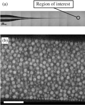
Figure 1: Top: Composite photograph of capillary tube. The scale bar is 500 $\mu$m. Bottom: 2D confocal image from experiment 55, with volume fraction $\phi_{\rm tot}=0.49$. The scale bar is 10 $\mu$m.

Our sample chambers are glass capillary tubes as shown in Fig. 1(top). The capillary tip was made using an automated pipette puller. To help the capillary tube fit onto a microscope slide, the large end of the capillary tip was cut off while ensuring not to break the thin end of the capillary tube. The thin end was often too thin, so it too was cut, leaving an opening a few microns in diameter. The shortened capillary tube was then dipped into a vial containing the colloidal suspension for 10 seconds or so, and the sample flows into the glass tube due to capillary forces. We use quick drying UV epoxy (Norland 81) to seal both ends of the tube and also to glue the tube to the slide. In fact, it is useful to cover the tip entirely with glue to ensure stability. The microscopy is not affected too much, as the sample and epoxy have similar indices of refraction (1.495 and 1.56 respectively). The result is a confined sample, such as shown in Fig 1(bottom), which can be studied at different locations to give different tube sizes. The capillary tubes vary slightly in radius as a function of length (slope of about $1^{\circ}$), and the slight taper does not seem to affect our overall results. The taper is slight enough that we cannot observe it in any of our confocal images. Due to the pipette puller protocol we used, the capillary tubes sag slightly, and so their cross-section is slightly elliptical rather than circular. This does not seem to influence our results and will be discussed further below. When the tubes are filled with the sample, some of the particles stick irreversibly to the tube walls due to van der Waals forces. This typically resulted in one complete layer of particles (of both sizes) coating the wall. During the course of our experiments, we do not observe any new particle sticking to the walls, nor do we observe any stuck particles becoming unstuck.

We use a confocal microscope (Visitech vt-Eye) to study our samples. In a confocal microscope, laser light is scanned across the fluorescent sample and excites the dye to emit a different color light. The emitted light passes through a pinhole to remove the out-of-focus light and then is measured by a detector, a photomultiplier tube in our microscope. The sample is quickly scanned in $x$ and $y$ to acquire a two-dimensional (2D) image. Then the microscope focus is adjusted to scan more 2D images at different depths $z$, thus building up a 3D image. Being able to create 3D images makes confocal microscopy a powerful tool for studying particle dynamics in the system. Each 3D scan takes about 2-3 seconds, and we typically take movies comprised of 400 of these 3D images. The particles are tracked in 3D using standard tracking techniques Crocker and Grier (1996); Dinsmore et al. (2001). Within each confocal image, the small and large particles are easy to tell apart [see Fig. 1(bottom)] and so we can distinguish between them in our data Narumi et al. (2011).

We have two control parameters, the tube radius and the volume fraction. Complete descriptions of how these are measured are given in the Appendix; here, we summarize the key points.

Our first control parameter is the tube radius. The positions of the particles give us an accurate idea where the tube surface is. However, the tubes have an elliptical cross-section rather than a circular cross section. We measure the major and minor axes $R_{\rm max}$ and $R_{\rm min}$ for each experiment. The ratio $R_{\rm max}/R_{\rm min}$ ranges from 1.14 to 1.39, with mean 1.24. Because we are concerned with confinement effects, we report our data in terms of $R_{\rm min}$ in general, although both radii are listed for all experiments in Table I. Note that we report the radii corresponding to the maximum positions of the observed particle centers: in general the particles at these maximum positions are the small ones (whose centers can get closer to the tube walls) and so the true tube sizes are larger by $a_{S}=0.532$ $\mu$m.

Our other key control parameter is the volume fraction $\phi$. We measure this in each data set by counting the numbers of small and large particles observed within a subvolume of the tube, and converting this to the volume fraction using the known particle sizes. Note that 1% uncertainties in the particle radii translate to 3% uncertainties of the volume fraction, and since each particle radius is uncertain, we have an overall systematic volume fraction uncertainty of at least 5% Poon et al. (2012).

In summary, our experimental method is to image different portions of the same tube in hopes to get a constant volume fraction with differing tube radii, and to study different tubes with different volume fractions to understand the role of volume fraction. In practice, we determine these variables when the data are post-processed, and report the measured values in Table I.

Expt	$\phi_{\rm tot}$	$R_{\rm min}$	$R_{\rm max}$	$\langle\Delta x^{2}\rangle$	$N_{\rm small}/N_{\rm tot}$
9b	0.19	11.1	14.9	4.8	0.45
9a	0.19	12.7	17.4	4.7	0.51
5a	0.20	10.5	14.2	2.9	0.37
12b	0.22	10.7	14.9	3.7	0.44
11b	0.22	8.5	11.3	2.2	0.37
63	0.43	6.5	7.4	0.43	0.43
54	0.45	10.9	13.2	0.86	0.33
52	0.46	13.1	15.9	1.0	0.18
55	0.49	12.8	15.4	0.91	0.18
56	0.49	14.3	17.2	0.70	0.14
51	0.50	17.1	20.7	0.99	0.07
62	0.51	8.6	9.8	0.29	0.17
65	0.53	8.8	10.1	0.22	0.16
64	0.54	7.8	8.9	0.11	0.22

Table 1: List of experiments, ordered by total volume fraction $\phi_{\rm tot}$. The volume fraction of the small particles can be determined by $\phi_{S}=\phi_{\rm tot}[1+((1-f)/f)(a_{L}/a_{S})^{3}]^{-1}$, where $f\equiv N_{\rm small}/N_{\rm tot}$. The volume fraction of the large particles is then $\phi_{L}=\phi_{\rm tot}-\phi_{S}$. The tube sizes $R_{\rm min}$ and $R_{\rm max}$ correspond to the maximum radii that the particle centers can reach; the physical tube walls are a distance $\approx a_{S}$ further away. The value of $\langle\Delta x^{2}\rangle$ given is for $\Delta t=100$ s, and corresponds to the information plotted in Figs. 2, 3.

3 Results

3.1 Motion slows in confined samples

By following the motion of all of the particles in 3D, we can observe how the motion depends on confinement. We quantify this by calculating the mean square displacement, defined as

$$\langle\Delta z^{2}\rangle=\langle[z(t+\Delta t)-z(t)]^{2}\rangle$$ (1)

where $\langle\Delta z^{2}\rangle$ is a function of the lag time $\Delta t$, and the angle brackets indicate an average over all times $t$ and all particles. Here we are considering the $z$ direction to be along the axis of the tube, primarily because this axis is perpendicular to the optical axis of the microscope and therefore has less position uncertainty. The data are plotted in Fig. 2, where each family of curves correspond to a different volume fraction. Within each family, the slower curves correspond to narrower tubes: confinement induces glassier behavior. To further quantify this, we consider the specific value of $\langle\Delta x^{2}\rangle$ at a lag time $\Delta t=100$ s (which is arbitrary but chosen to match prior work Nugent et al. (2007)). This value is plotted as a function of minimum tube radius $R_{\rm min}$ in Fig. 3. The different symbols correspond to different ranges of volume fractions, and in general within each range, smaller tubes correspond to slower motion. Plotting the data against $R_{\rm max}$, $(R_{\min}+R_{\max})/2$, or $\sqrt{R_{\rm min}R_{\rm max}}$ does not change the overall appearance of this graph significantly. It is intriguing to note that the magnitude of the effect is less significant than was seen in similar experiments with parallel plates Nugent et al. (2007). Here, the strongest influence of confinement is to lower mobility by a factor of $\sim 3$ (for circles, squares, and triangles in Fig. 3). With parallel plates, mobility was lowered by a factor of $\sim 40$ for data with $\phi\approx 0.46$ Nugent et al. (2007), a volume fraction in the same range as our cylindrical data. We are unsure why the two experiments differ in the magnitude of mobility reduction.

Figure 2: Mean square displacements in the $z$ direction (along the cylinder axis). Each family of curves is labeled at left by the volume fraction, and at right by the values of the minimum cylinder radius (in $\mu$m). For each curve, the volume fraction is within $0.02$ of the labeled value.

Figure 3: The value of $\langle\Delta x^{2}\rangle$ at the time scale $\Delta t=100$ s, plotted as a function of the cylinder minimum radius $R_{\rm min}$. The symbols indicate the volume fraction: circles are $\phi=0.21\pm 0.02$, squares are $\phi=0.45\pm 0.02$, diamonds are $\phi=0.49\pm 0.01$, and triangles are $\phi=0.53\pm 0.02$. The circles correspond to the dotted lines in Fig. 2, the squares correspond to the dashed lines, and the triangles correspond to the solid lines. See Table I for a full listing of all volume fractions, mobility values, and other details.

3.2 Motion is slower near walls

Microscopy allows us to spatially resolve details of the motion. If confinement-induced slowing is a finite size effect, then the motion might be spatially homogeneous: the whole sample feels that it is small He et al. (2007); Richert (2011). If instead the confinement-induced slowing is an interfacial effect (due to the sample-wall interface), then particle motion would depend on where each particle is relative to the boundary. Of course, both effects could be present simultaneously Morineau et al. (2002). We check this by plotting the particle mobility $\langle\Delta r^{2}\rangle$ as a function of the distance $s$ to the nearest wall in Fig. 4(a). It is immediately apparent that particles move slower when they are close to the wall ($s\rightarrow 0$), and a plateau value for the mobility isn’t reached until several particle radii into the sample. Note that we are using the full 3D mobility $\langle\Delta r^{2}\rangle=\langle\Delta x^{2}+\Delta y^{2}+\Delta z^{2}\rangle$, for a fixed lag time $\Delta t=30$ s (for which we have more statistics), and now the angle brackets indicate an average over those particles with the specific value of $s$. The value of $s$ is based on the initial position of the particle, at time $t$ rather than $t+\Delta t$. It is probable that the mobility near the wall is very slightly enhanced, due to particles which diffuse away from the wall during $\Delta t$ and thus enhance their mobility Eral et al. (2010). The different curves are for small and large particles as indicated. Not surprisingly, the smaller particles are more mobile than the large ones. Our directly observed gradient in mobility is similar to that inferred from experiments on small molecule glasses He et al. (2005, 2007); Le Quellec et al. (2007), polymer glasses Ellison and Torkelson (2003), and seen directly in simulations Kob et al. (2000); Scheidler et al. (2002); Teboul and Simionesco (2002). Our data show that the mobility changes over a distance of several particle diameters.

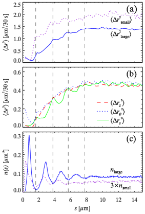
Figure 4: (Color online) (a) Mobility as a function of distance $s$ from the wall, for the small particles and large particles as indicated. (b) Mobility for the large particles only, for the components of motion as indicated. (c) Number densities of the small and large particles. Note that the number density of the small particles has been multiplied by four. In all panels, the vertical dashed lines correspond to the local minima of $n_{\rm large}$. They are spaced approximately 2.04 $\mu$m apart. The data are from experiment 51 with $\phi_{\rm tot}=0.50$ and $R_{\rm min}=17.1$ $\mu$m; see Table I for other details.

A second feature of the data of Fig. 4(a) is that the curves oscillate. The oscillations are related to the fluctuations of the particle number density, as seen by comparing Fig. 4(a) to Fig. 4(c). The latter shows the fluctuations of the number density of large and small particles (solid and dotted lines, respectively). The mobility data in Fig. 4(a) are anticorrelated with $n_{\rm large}(s)$: the local minima of $n_{\rm large}(s)$ are indicated by the vertical dashed lines, and correspond to local maxima of $\langle\Delta r^{2}\rangle$. The influence of $n_{\rm small}$ is not seen, probably because the number fraction of small particles is much less than that of the large particles ($N_{\rm small}/N_{\rm large}=0.07$ for these data). The anticorrelation between number density and mobility matches what has been seen in prior work on confined samples Nugent et al. (2007); Edmond et al. (2012).

Further insight into the mobility is found by splitting $\langle\Delta r^{2}\rangle$ into components parallel to the tube ($z$ direction), tangential to the tube wall ($\theta$ direction), and in the radial direction ($s$ direction). These components of mobility are shown in Fig. 4(b). Here it is apparent that the radial mobility is the most influenced by the oscillations of $n_{\rm large}(s)$. Again, this is the same result seen before with flat walls Nugent et al. (2007). The particles at the maxima of $n_{\rm large}(s)$ appear to be at favorable positions and their mobility is reduced, whereas those at the minima are in less favorable positions with higher mobility. Motions in the $z$ and $\theta$ directions are along contours of constant mean $n$ and do not fluctuate with $n(s)$.

All of the results of Fig. 4 are qualitatively replicated in Fig. 5, which is data from a smaller radius tube ($R_{\min}=7.8$ $\mu$m compared to $R_{\rm min}=17.1$ $\mu$m) and volume fraction only slightly larger than that of Fig. 4 ($\phi_{\rm tot}=0.54$ compared to 0.50). In Fig. 5(a), the mobility is lower near the boundary, lower for large particles, and oscillates with higher mobility corresponding to minima of $n_{\rm large}(s)$. The data for the components [Fig. 5(b)] are noisier due to less statistics in the smaller tube, but again $\langle\Delta r_{s}^{2}\rangle$ shows a stronger anticorrelation with $n_{\rm large}(s)$. The oscillations of $n_{\rm large}(s)$ in Fig. 5(c) are more complex than those seen in Fig. 4(c), probably due to packing constraints of a smaller tube.

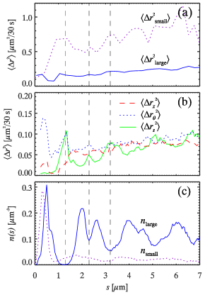
Figure 5: (Color online) (a) Mobility as a function of distance $s$ from the wall, for the small particles and large particles as indicated. (b) Mobility for the large particles only, for the components of motion as indicated. (c) Number densities of the small and large particles. In all panels, the vertical dashed lines correspond to some of the local minima of $n_{\rm large}$. The data are from experiment 64 with $\phi_{\rm tot}=0.54$ and $R_{\rm min}=7.8$ $\mu$m; see Table I for other details.

4 Conclusions

Our results – in particular Figs. 4(a) and 5(a) – suggest that the slower motion of confined colloidal samples is due to an interfacial effect, where particles near the sample walls are slowed. This agrees with a prior observation that colloidal particle motion is slower near rougher walls Edmond et al. (2010), a result demonstrating that the nature of the confining walls plays a role and not merely the finite size of the sample chamber. It is unlikely this is merely a hydrodynamic effect, as the magnitude of such an effect would only be a factor of $\sim 2-4$ in mobility and would not depend on $R_{\rm min}$ Eral et al. (2010); Edmond et al. (2012).

The clear gradient seen in Figs. 4(a) and 5(a) was not seen in prior work where colloids were confined between parallel walls Nugent et al. (2007). It may be that the influence of confinement is stronger in the cylindrically confined case: between parallel walls, there are two unconfined directions, whereas in the cylinder there is only one unconfined direction Barut et al. (1998). Another possibility is that the curvature of the cylindrical walls introduces an effect not present with flat walls. These geometrical differences are the only major differences between the experiments in this paper and those published earlier. As noted in Sec. 3.1, the other observed difference is that the slowing of motion in cylindrically confined samples (Fig. 3) is less pronounced compared to the observations between parallel plates Nugent et al. (2007). This is counterintuitive given the argument above that cylindrical confinement is “stronger” than parallel-plate confinement. This trend is the opposite of that seen for small molecule liquids Barut et al. (1998). Future experiments may be able to elaborate on the question for colloids: at one extreme, particle motion could be studied in a half-infinite system near a wall, whereas at the other extreme, particle motion could be studied in a spherical pore. The data presented in this paper suggest that changing the dimensionality of the confinement in this way can result in interesting and qualitatively distinct behavior, in other words, enhancing a mobility gradient near walls while diminishing the overall confinement effect.

Our results also imply that flowing colloidal suspensions through small cylindrical tubes will be harder for smaller tube radii. Additionally, the decrease in mobility near the walls perhaps implies an increase in the apparent viscosity of the sample near the walls, thus modifying the flow velocity profile in a nontrivial fashion.

Note that we do not see any quantization effects: we do not see any particular change in the dynamics at any special ratios of particle sizes to tube sizes. This is in contrast to some theoretical predictions Mittal et al. (2008); Desmond and Weeks (2009); Lang et al. (2010). However, our data are only at a limited number of tube sizes, as shown in Fig. 3; our tubes are elliptical in cross section and so the ratio of particle size to tube size is not a constant for any given data set; and it is likely that such quantization effects are more subtle than we would be able to see in an experiment.

Appendix

We explain in more detail how our experimental parameters are measured. In each case, we prepare samples and take data, measuring the tube radii and volume fraction from the data.

Tube radius: As noted in Sec. 2, the tubes do not typically have a circular cross-section. Also, in general, the images of the tube are not precisely aligned with the $xyz$ laboratory reference frame. To determine the radius, the position data are first rotated by $0-4^{\circ}$ around the $x$ and $y$ axes as necessary so that the $z$ axis of the data corresponds with the tube axis. (Note that the $z$ axis is not the optical axis of the microscope; rather, the $z$ axis is within a few degrees of perpendicular to the optical axis.) Then the data are projected onto the $xy$ plane and their center of mass is found. The $x,y$ coordinates are converted to $r,\theta$ and the maximum $r$ is found as a function of $\theta$. Following the procedure of Eral et al., in order to smooth the measured contour we fit $r(\theta)$ to a Fourier series up to $m=4$ modes Eral et al. (2010). The function $r(\theta)$ is found to be well-described by an ellipse in all cases, and accordingly it is easy to determine the major and minor axes.

Volume fraction: For our experiments, we take movies from different portions of several tubes. Ideally each tube is filled with a sample of homogeneous volume fraction, but in practice the volume fraction varies slightly from region to region. Additionally, defining volume fractions in confined sample chambers is a little problematic as the concentration is inherently smaller at the walls simply due to packing constraints Desmond and Weeks (2009) even if the interparticle spacing is spatially homogeneous. To define volume fraction, we integrate the $r(\theta)$ data described in the previous paragraph to determine the cross sectional area (adding on $a_{S}$ to determine the physical wall boundary). The length of the observed region is known, so therefore we know the volume $V_{\rm tot}$ of the tube that is imaged. Likewise we know the numbers of the small and large particles $N_{S}$ and $N_{L}$ that are in the image, and so the volume fraction can be determined from $(N_{S}V_{S}+N_{L}V_{L})/V_{\rm tot}$ in terms of the individual particle volumes $V_{S}$ and $V_{L}$. $V_{S}\sim a_{s}^{3}$ and likewise for $V_{L}$, so 1% uncertainties in the particle radii lead to 3% uncertainties of the volume fraction. Since each particle radius is uncertain, we have an overall systematic volume fraction uncertainty of at least 5% Poon et al. (2012). There is also some uncertainty between samples as the different samples are observed to have different number ratios of small and large particles (see Table I), and so errors in small and large particle radii will affect the different volume fraction calculations in different amounts. Encouragingly, visual inspection of the images suggests that the calculated volume fractions listed in Table I are at least qualitatively in correct order. Samples with volume fractions within 0.02 of each other appear visually to be the same volume fraction, and samples with greater differences are visually distinct.

References

- Götze and Sjögren (1992) W. Götze, and L. Sjögren, Rep. Prog. Phys. 55, 241–376 (1992).
- Ediger et al. (1996) M. D. Ediger, C. A. Angell, and S. R. Nagel, J. Phys. Chem. 100, 13200–13212 (1996).
- Debenedetti and Stillinger (2001) P. G. Debenedetti, and F. H. Stillinger, Nature 410, 259–267 (2001).
- Cavagna (2009) A. Cavagna, Physics Reports 476, 51–124 (2009).
- Dyre (2006) J. C. Dyre, Rev. Mod. Phys. 78, 953–972 (2006).
- Berthier et al. (2011) L. Berthier, P. Chaudhuri, C. Coulais, O. Dauchot, and P. Sollich, Phys. Rev. Lett. 106, 120601 (2011).
- Roland et al. (2005) C. Roland, S. Hensel-Bielowka, M. Paluch, and R. Casalini, Rep. Prog. Phys. 68, 1405–1478 (2005).
- Alba-Simionesco et al. (2006) C. Alba-Simionesco, B. Coasne, G. Dosseh, G. Dudziak, K. E. Gubbins, R. Radhakrishnan, and M. Sliwinska-Bartkowiak, J. Phys.: Cond. Matt. 18, R15–R68 (2006).
- Hunter and Weeks (2012) G. L. Hunter, and E. R. Weeks, Rep. Prog. Phys. 75, 066501 (2012).
- Ernst et al. (1991) R. M. Ernst, S. R. Nagel, and G. S. Grest, Phys. Rev. B 43, 8070–8080 (1991).
- Charbonneau et al. (2012) B. Charbonneau, P. Charbonneau, and G. Tarjus, Phys. Rev. Lett. 108, 035701 (2012).
- Roth and Dutcher (2005) C. B. Roth, and J. R. Dutcher, J. Electroanalytical Chem. 584, 13–22 (2005).
- Alcoutlabi and McKenna (2005) M. Alcoutlabi, and G. B. McKenna, J. Phys.: Cond. Matt. 17, R461–R524 (2005).
- Richert (2011) R. Richert, Ann. Rev. Phys. Chem. 62, 65–84 (2011).
- Marshall and Zukoski (1990) L. Marshall, and C. F. Zukoski, J. Phys. Chem. 94, 1164–1171 (1990).
- Segrè et al. (1995) P. N. Segrè, S. P. Meeker, P. N. Pusey, and W. C. K. Poon, Phys. Rev. Lett. 75, 958–961 (1995).
- Poon et al. (1996) W. C. K. Poon, S. P. Meeker, P. N. Pusey, and P. N. Segrè, J. Non-Newt. Fluid Mech. 67, 179–189 (1996).
- Cheng et al. (2002) Z. Cheng, J. Zhu, P. M. Chaikin, S.-E. Phan, and W. B. Russel, Phys. Rev. E 65, 041405 (2002).
- Pusey and van Megen (1986) P. N. Pusey, and W. van Megen, Nature 320, 340–342 (1986).
- Zaccarelli et al. (2009) E. Zaccarelli, C. Valeriani, E. Sanz, W. Poon, M. Cates, and P. Pusey, Phys. Rev. Lett. 103, 135704 (2009).
- Pusey et al. (2009) P. N. Pusey, E. Zaccarelli, C. Valeriani, E. Sanz, W. C. K. Poon, and M. E. Cates, Phil. Trans. Roy. Soc. A 367, 4993–5011 (2009).
- Nugent et al. (2007) C. R. Nugent, K. V. Edmond, H. N. Patel, and E. R. Weeks, Phys. Rev. Lett. 99, 025702 (2007).
- Edmond et al. (2010) K. V. Edmond, C. R. Nugent, and E. R. Weeks, Euro. Phys. J. - Special Topics 189, 83–93 (2010).
- Edmond et al. (2012) K. V. Edmond, C. R. Nugent, and E. R. Weeks, Phys. Rev. E 85, 041401 (2012).
- Sarangapani and Zhu (2008) P. S. Sarangapani, and Y. Zhu, Phys. Rev. E 77, 010501 (2008).
- Sarangapani et al. (2011) P. S. Sarangapani, A. B. Schofield, and Y. Zhu, Phys. Rev. E 83, 030502 (2011).
- Eral et al. (2009) H. B. Eral, D. van den Ende, F. Mugele, and M. H. G. Duits, Phys. Rev. E 80, 061403 (2009).
- Morineau et al. (2002) D. Morineau, Y. Xia, and C. Alba-Simionesco, J. Chem. Phys. 117, 8966–8972 (2002).
- Serghei et al. (2010) A. Serghei, D. Chen, D. H. Lee, and T. P. Russell, Soft Matter 6, 1111–1113 (2010).
- Kob et al. (2000) W. Kob, P. Scheidler, and K. Binder, Europhys. Lett. 52, 277–283 (2000).
- Scheidler et al. (2002) P. Scheidler, W. Kob, and K. Binder, Europhys. Lett. 59, 701–707 (2002).
- Harris and Erickson (1980) W. F. Harris, and R. O. Erickson, Journal of Theoretical Biology 83, 215–246 (1980).
- Pittet et al. (1996) N. Pittet, P. Boltenhagen, N. Rivier, and D. Weaire, Europhys. Lett. pp. 547–552 (1996).
- Moon et al. (2004) J. H. Moon, S. Kim, G.-R. Yi, Y.-H. Lee, and S.-M. Yang, Langmuir 20, 2033–2035 (2004).
- Li et al. (2005) F. Li, X. Badel, J. Linnros, and J. B. Wiley, J. Am. Chem. Soc. 127, 3268–3269 (2005).
- Tymczenko et al. (2008) M. Tymczenko, L. F. Marsal, T. Trifonov, I. Rodriguez, F. Ramiro-Manzano, J. Pallares, A. Rodriguez, R. Alcubilla, and F. Meseguer, Adv. Mater. 20, 2315–2318 (2008).
- Lohr et al. (2010) M. A. Lohr, A. M. Alsayed, B. G. Chen, Z. Zhang, R. D. Kamien, and A. G. Yodh, Phys. Rev. E 81, 040401 (2010).
- Eral et al. (2010) H. B. Eral, J. M. Oh, D. van den Ende, F. Mugele, and M. H. G. Duits, Langmuir 26, 16722–16729 (2010).
- Valley et al. (2007) D. T. Valley, S. A. Rice, B. Cui, H. M. Ho, H. Diamant, and B. Lin, J. Chem. Phys. 126, 134908 (2007).
- Wonder et al. (2011) E. Wonder, B. Lin, and S. A. Rice, Phys. Rev. E 84, 041403 (2011).
- Alder and Wainwright (1957) B. J. Alder, and T. E. Wainwright, J. Chem. Phys. 27, 1208–1209 (1957).
- Woodcock and Angell (1981) L. V. Woodcock, and C. A. Angell, Phys. Rev. Lett. 47, 1129–1132 (1981).
- Speedy (1998) R. J. Speedy, Molecular Physics 95, 169–178 (1998).
- Antl et al. (1986) L. Antl, J. W. Goodwin, R. D. Hill, R. H. Ottewill, S. M. Owens, S. Papworth, and J. A. Waters, Colloids and Surfaces 17, 67–78 (1986).
- Yethiraj and van Blaaderen (2003) A. Yethiraj, and A. van Blaaderen, Nature 421, 513–517 (2003).
- Crocker and Grier (1996) J. C. Crocker, and D. G. Grier, J. Colloid Interf. Sci. 179, 298–310 (1996).
- Dinsmore et al. (2001) A. D. Dinsmore, E. R. Weeks, V. Prasad, A. C. Levitt, and D. A. Weitz, App. Optics 40, 4152–4159 (2001).
- Narumi et al. (2011) T. Narumi, S. V. Franklin, K. W. Desmond, M. Tokuyama, and E. R. Weeks, Soft Matter 7, 1472–1482 (2011).
- Poon et al. (2012) W. C. K. Poon, E. R. Weeks, and C. P. Royall, Soft Matter 8, 21–30 (2012).
- He et al. (2007) F. He, L. M. Wang, and R. Richert, Euro. Phys. J. - Special Topics 141, 3–9 (2007).
- He et al. (2005) F. He, L. M. Wang, and R. Richert, Phys. Rev. B 71, 144205 (2005).
- Le Quellec et al. (2007) C. Le Quellec, G. Dosseh, F. Audonnet, N. Brodie-Linder, C. Alba-Simionesco, W. Häussler, and B. Frick, Euro. Phys. J. - Special Topics 141, 11–18 (2007).
- Ellison and Torkelson (2003) C. J. Ellison, and J. M. Torkelson, Nature Materials 2, 695–700 (2003).
- Teboul and Simionesco (2002) V. Teboul, and C. A. Simionesco, J. Phys.: Cond. Matt. 14, 5699–5709 (2002).
- Barut et al. (1998) G. Barut, P. Pissis, R. Pelster, and G. Nimtz, Phys. Rev. Lett. 80, 3543–3546 (1998).
- Mittal et al. (2008) J. Mittal, T. M. Truskett, J. R. Errington, and G. Hummer, Phys. Rev. Lett. 100, 145901 (2008).
- Desmond and Weeks (2009) K. W. Desmond, and E. R. Weeks, Phys. Rev. E 80, 051305 (2009).
- Lang et al. (2010) S. Lang, V. Boţan, M. Oettel, D. Hajnal, T. Franosch, and R. Schilling, Phys. Rev. Lett. 105, 125701 (2010).