Scaling relations of metallicity, stellar mass, and star formation rate in metal-poor starbursts: II. Theoretical models

Abstract

Scaling relations of metallicity (O/H), star formation rate (SFR), and stellar mass ($M_{\rm star}$) give important insight on galaxy evolution. They are obeyed by most galaxies in the Local Universe and also at high redshift. In a companion paper, we compiled a sample of $\sim$1100 galaxies from redshift 0 to $\ga 3$, spanning almost two orders of magnitude in metal abundance, a factor of $\sim 10^{6}$ in SFR, and of $\sim 10^{5}$ in stellar mass. We have characterized empirically the star-formation “main sequence” (SFMS) and the mass-metallicity relation (MZR) for this sample, and also identified a class of low-metallicity starbursts, rare locally but more common in the distant universe. These galaxies deviate significantly from the main scaling relations, with high SFR and low metal content for a given $M_{\rm star}$. In this paper, we model the scaling relations and explain these deviations from them with a set of multi-phase chemical evolution models based on the idea that, independently of redshift, initial physical conditions in a galaxy’s evolutionary history can dictate its location in the scaling relations. Our models are able to successfully reproduce the O/H, $M_{\rm star}$, and SFR scaling relations up to $z\lower 2.15277pt\hbox{$\;\buildrel>\over{\sim}\;$}3$, and also successfully predict the molecular cloud fraction as a function of stellar mass. These results suggest that the scaling relations are defined by different modes of star formation: an “active” starburst mode, more common at high redshift, and a quiescent “passive” mode that is predominant locally and governs the main trends.

1 Introduction

Scaling relations of metallicity O/H, stellar mass $M_{\rm star}$, and star-formation rate (SFR) are powerful tools for probing galaxy evolution across cosmic time. The star-formation “main sequence” (SFMS) connects current star formation with a galaxy’s stellar mass (Noeske et al., 2007; Salim et al., 2007; Schiminovich et al., 2007; Bauer et al., 2011), and the mass-metallicity relation (MZR) links stellar mass with metal content (Tremonti et al., 2004). Recently, Mannucci et al. (2010) found that SFR influences a galaxy’s position in the MZR, and introduced the “Fundamental Metallicity Relation” (FMR), which reduces the scatter in their local sample of galaxies to $\sim$0.06 dex (see also Lara-López et al., 2010).

There is, however, evidence that galaxies outside the Local Universe ($z\ga 1$) do not follow the same SFMS and MZR. The FMR successfully fits Lyman Break Galaxies (LBGs) up to $z\la 2$, but fails for higher redshifts (Mannucci et al., 2010). The SFMS has similar slopes with increasing redshift but larger offsets (Bauer et al., 2011); for a given stellar mass, a more distant galaxy has a higher SFR. Starbursts at all redshifts tend to lie above the SFMS, with high specific SFRs (sSFRs), and too much luminosity (or stellar mass) for their metallicity (e.g., Hoyos et al., 2005; Rosario et al., 2008; Salzer et al., 2009; Peeples et al., 2009). These high-SFR outliers have been attributed to merger-induced episodes of star formation that tend to be short-lived and intense (e.g., Rodighiero et al., 2011), while the SFMS is followed by more passively evolving galaxies that form stars over longer times.

Here we propose that mergers may not be directly responsible for producing the starbursts that depart from the general SFR-mass-metallicity relations. Instead, independently of their cause, different modes of star formation arising from different initial sizes and densities, may be driving the deviations. Active star formation that takes place in compact regions with dense gas has distinct properties from a more passive mode in larger, more tenuous regions; in the former, dynamical times are shorter, infrared luminosities and SFRs are higher, and molecular fractions are more elevated (Hirashita & Hunt, 2004). In the Local Universe, compact sizes and high-density gas characterize metal-poor starbursts which occur in dwarf galaxies with high SFRs (Hunt & Hirashita, 2009). At high redshift, starbursts also tend to be compact in size ($\la 4$ kpc in diameter, Tacconi et al., 2006, 2008; Toft et al., 2009). Compactness also shapes spectral energy distributions causing them to peak at shorter wavelengths, because the dust heated by a compact starburst tends to be warmer (Chanial et al., 2007; Groves et al., 2008; Melbourne et al., 2009).

Active star formation is expected to also be characterized by high ionization parameters because of the compact and dense nature of the active SF complexes. Figure 1 shows the ionization parameters $U$ of a sample of low-metallicity Blue Compact Dwarf galaxies (BCDs) taken from Hunt & Hirashita (2009). The ionization parameter of the Hii regions increases with ionized gas density $n_{e}$; for this sample the significance of the correlation is $>$99%. Because the size of the Hii region is inversely correlated with density (e.g., Hunt & Hirashita, 2009), $U$ depends almost linearly on $n_{e}$. Anomalous Hii-region excitation is frequently found in some high-redshift galaxy populations (e.g., Hammer et al., 1997; Liu et al., 2008; Brinchmann et al., 2008; Erb et al., 2010). Excluding a contribution from a weak active galactic nucleus, it is likely that this excitation results from the extreme physical conditions of the active SF mode, with dense ionized gas and high SFR surface densities (Liu et al., 2008). Such properties naturally arise in dense and compact Hii regions with particularly hard radiation fields. Thus, the anomalous excitation and high ionization parameters observed in high-redshift samples may also be signatures of active starbursts which occur in a chemically unenriched interstellar medium (ISM).

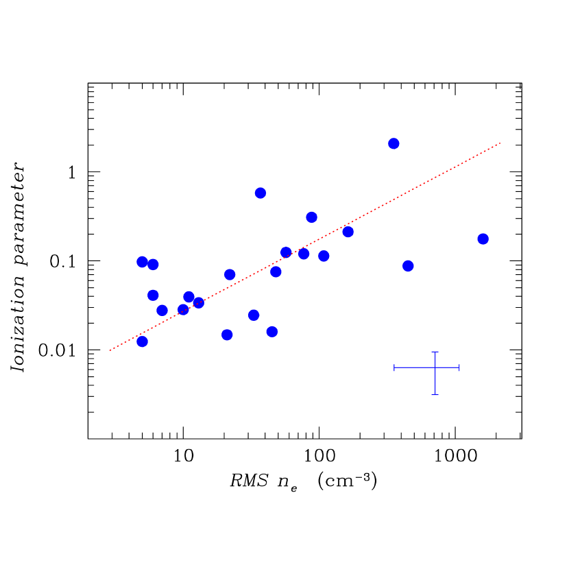
Figure 1: Ionization parameter vs. root-mean-square electron density of Hii regions in a sample of BCDs from Hunt & Hirashita (2009). The typical error bars are shown in the lower right corner. The dotted line shows the best-fit correlation.

Besides compact, dense star-forming regions, and possibly high-ionization parameters for the nebular gas, there are further, probably related, properties shared by some galaxy populations in the nearby universe and those at high redshift. As discussed in Hunt et al. (2012, hereafter Paper I), some metal-poor BCDs deviate significantly from the SFMS and the MZR; they are characterized by high SFRs, high sSFRs, and are situated in the SFMS and the MZR in the same region as the $z=3$ LBGs. For a given (sub-solar) metallicity, these galaxies can have an excess of stellar mass of two orders of magnitude, and a factor of $\sim 10$ excess SFR for a given mass. Some of the “Green Peas” and Luminous Compact Galaxies (LCGs) at $z\sim 0.1-0.4$ selected by Cardamone et al. (2009) and Izotov et al. (2011) also lie in the same regions of the SFMS and the MZR and show similar excesses. Similar physical conditions seem to occur at all redshifts, but different galaxy populations are observed at different redshifts because of how they are selected. Since extreme starbursts are rare locally, but more common at high redshift, it could be that different modes of star formation drive the scaling relations of stellar mass, metallicity, and SFR we observe.

In this paper, we present semi-analytical models which are aimed at understanding how different modes of star formation affect the SFMS and MZR. In particular, we focus on metal-poor galaxies with high SFRs, which are generally more massive than would be expected given their metal abundance. We develop three families of initial conditions for star formation and compare model predictions with several samples comprising $\la$ 1100 nearby metal-poor dwarf galaxies, intermediate redshift and high-redshift galaxy populations (see Paper I). The initial conditions are designed to embrace the active/passive (compact$+$dense/extended$+$diffuse) modes of star formation and thus distinguish the active starburst modes from more passive quiescent ones. The questions we aim to address are:

1. Why can both high and low SFRs be observed at the same metallicity?

2. What are the specific conditions which distinguish starbursts (active SF mode) from quiescent star formation (passive mode)?

3. Is there a connection between active dwarfs and high-z starbursts in terms of their scaling relations (SFMS, MZR, FMR)?

The paper is organized as follows: in Sect. 2 we briefly describe the samples we have compiled and how we calculate the stellar mass. The sample is more completely described in Paper I. In Sect. 3, we discuss our semi-analytical models which consider different sets of initial conditions in order to mimic the starburst and quiescent modes of star formation. Comparisons of model predictions with observations are given in Sect. 4, and Sect. 5 discusses the relation of the gas-to-stellar mass ratio and metal abundance. In Sect. 6 we describe possible similarities between nearby and distant starbursts, and how the scaling relations we observe and successfully model can shed light on how galaxies evolve.

2 The sample and the observables

Our sample was compiled on the basis of three “pseudo-observational” parameters: SFR, metal abundance [as defined by the nebular oxygen abundance, 12$+\log$(O/H)], and stellar mass, $M_{\rm star}$. We included only galaxies with these data either already published, or for which we could derive the quantities ourselves (in particular the stellar masses). These criteria were met by galaxies from five samples at $z\sim 0$: 21 nearby dwarf irregular galaxies (dIrr) published by Lee et al. (2006, hereafter “dIrr”), 129 of the 11 Mpc distance-limited sample of nearby galaxies (11HUGS, LVL: Kennicutt et al., 2008), and 89 BCDs in the samples presented by Engelbracht et al. (2008), Fumagalli et al. (2010), and Hunt et al. (2010). Seven galaxy samples at higher redshifts also have the necessary data: the “Green Pea” compact galaxies identified by the Galaxy Zoo team at $z\sim 0.1-0.3$ (Cardamone et al., 2009), the LCG sample at $z\sim 0.1-0.6$ selected by Izotov et al. (2011), LBGs at $z\sim 1$ (Shapley et al., 2005a), $z\sim 2$ (Shapley et al., 2004; Erb et al., 2006), and $z\sim 3$ (Maiolino et al., 2008; Mannucci et al., 2009). When stellar masses were not available in the literature, we determined stellar masses from IRAC photometry as discussed below, and in detail in Paper I.

Altogether, we consider in the analysis 1070 galaxies from $z\sim 0$ to $z\sim 3$ with the requisite three quantities of SFR, 12$+\log$(O/H), and $M_{\rm star}$. Except for the galaxies with $z\ga 1$ (Shapley et al., 2004, 2005a; Erb et al., 2006; Maiolino et al., 2008; Mannucci et al., 2009) and a few of the LVL galaxies (Marble et al., 2010), metallicities for all galaxies are determined by the “direct” (electron temperature) method (e.g., Izotov et al., 2007) since the samples are defined by requiring detections of Oiii$\lambda$4363. SFRs are derived from H$\alpha$ luminosities corrected for extinction; in a few BCDs, the IR luminosity gave higher SFRs, so we used the higher value. SFRs using the Kennicutt (1998) conversion are reported to the Chabrier (2003) Initial Mass Function (IMF). Paper I gives a detailed description of the sample.

We calculated the stellar masses for the local samples (dIrr, BCDs, 11HUGS/LVL) from Spitzer/IRAC observations at 4.5 µm (and when available also 3.6 µm). We based our method on that used by Lee et al. (2006) who analyzed sub-solar metallicity models from Bell & de Jong (2001) to derive stellar mass-to-light (M/L) as a linear function of $B-K$. The advantage of using 4.5 µm to measure stellar masses is that it minimizes variations in the M/L ratio (e.g., Jun & Im, 2008), because the ratio depends only weakly on age and metallicity, and dust extinction is negligible.

However, before calculating the masses, we subtracted the nebular continuum and recombination line emission from the broadband 4.5 µm photometry. Nebular emission in metal-poor starbursts, both in the continuum and lines, can significantly affect photometry (e.g., Reines et al., 2010; Atek et al., 2011), and thus have a potentially strong impact on the inferred stellar masses. This can be especially important in the 4.5 µm band (Smith & Hancock, 2009). Hence, before applying the formalism of Lee et al. (2006), from the SFR we have inferred the strength of Br$\alpha$ emission and the nebular continuum in the 4.5 µm IRAC band, and subtracted it from the observed flux. Then, following Lee et al. (2006), 4.5 µm luminosity was converted to stellar mass with a M/L corrected for different ages and metallicities with a color correction $B-$[4.5]. All stellar masses are scaled to the Chabrier (2003) IMF.

The final combined sample covers a $\sim 10^{5}$ range in stellar mass, a factor of $\sim 10^{6}$ in SFR, and 2 orders of magnitude in oxygen abundance. The metallicities are generally (formally) quite accurate, with uncertainties on the direct method of $\;\buildrel<\over{\sim}\;$0.05 dex, but the strong-line method and its comparison with the direct method of determining abundances from electron temperatures are compromised by differences in calibration that can be quite large (e.g., Kewley & Ellison, 2008, see also Paper I). The SFRs suffer from the typical uncertainties of H$\alpha$ measurements and the uncertain extinction corrections, and the uncertainty is expected to be $\;\buildrel<\over{\sim}\;$30%. The uncertainties on the stellar masses are typically 0.1 dex (30%), but can be as high as 50-70% when there are unusual colors. In any case, the large dynamic range of our combined sample should overwhelm any uncertainties on individual galaxy parameters. More details are given in Paper I.

2.1 Metal-poor starbursts

Since we are interested in deviations from the scaling relations, particularly those of galaxies with high SFR, relatively high mass, and low metallicity, in Paper I we quantified a “low-metallicity starburst”. Because deviations from the MZR become significant at abundances at or below 12$+\log$(O/H)$\sim$8.0, we consider this as a threshold below which a galaxy can be considered ”low-metallicity”. Deviations from the SFMS and the MZR become noticeable at SFRs of $\sim 0.6$ $M_{\odot}$ yr^-1. Hence we loosely define low-metallicity starburst (LMS) as a galaxy with a SFR $\geq$0.6 $M_{\odot}$ yr^-1and with 12$+\log$(O/H)$\leq$8.0. This is a rather arbitrary label, but one that enables us to identify the galaxies most likely to deviate from the scaling relations (see Paper I). Among the various samples, the LMSs are relatively rare: 2% of the LVL fall into this category; $\sim$11% of the BCDs; 22% of the LCGs; and $\sim$27% of the high-$z$ LBGs. Clearly selection effects (e.g., emission line surveys for the BCDs, emission-line flux for the LCGs) make it more likely for a galaxy to be a LMS, but there is some indication that LMSs are more common at high redshift.

3 Theoretical Models

Here we develop the models with which we explore the idea that particular initial physical conditions in a galaxy’s evolutionary history can change its location in the scaling relations independently of redshift. In particular, we have devised three sets of starting parameters which dictate the subsequent evolution of the galaxy, and which encompass the observed distinctions between “active” and “passive” star formation (see Sect. 1). The models and the different initial conditions are described below.

Although our models have been shown to realistically approximate the chemical evolution in nearby galaxies (e.g., Mollá et al., 1996, 1997; Mollá & Díaz, 2005; Magrini et al., 2007), in those models gas accretion has been considered. Here, as a first approximation, we use a closed box in which neither infall of pristine gas nor outflow of metal-enriched material are contemplated. Despite these significant limitations, which will be addressed in future work, we will show below that our models are remarkably successful in predicting the details of the SFMS and MZR scaling relations. They also are consistent with the observed gas fractions both locally and at high redshift.

3.1 The multiphase chemical evolution model

The models developed for the present work have been renamed as MICE (Multiphase Interstellar medium Chemical Evolution) models. MICE models adopted here are a generalization of the multi-phase model by Ferrini et al. (1992), originally built for the solar neighborhood, and subsequently extended to the entire Galaxy (Ferrini et al., 1994), and to other disk galaxies (e.g., Mollá et al., 1996, 1997; Mollá & Díaz, 2005; Magrini et al., 2007, 2009). We refer to those papers for a detailed description of the general formalism. The main differences of the models presented here relative to those used to describe the chemical evolution of disk galaxies are: i) MICE models are one-zone models, with a single galactic component and without infall or outflow processes; ii) no radial variations are considered, so that a uniform evolution is assumed for the whole galaxy.

Each galaxy is composed of four components: diffuse gas ($g$), clouds ($c$), stars ($s$) and stellar remnants ($r$). At $t=0$ all the mass of the galaxy is in the form of diffuse gas; subsequently, the mass fractions are modified by several conversion processes. The main processes considered in the model are: (i) conversion of diffuse gas into clouds; (ii) formation of stars from clouds and (iii) disruption of clouds by previous generations of massive stars; (iv) evolution of stars into remnants and return of a fraction of their mass to the diffuse gas.

We describe in the following the main equations of the model. Stars form by cloud-cloud collisions with a rate $P_{\mathit{sf}}$ and by the interactions of massive stars with clouds with rate $P_{i}$ (induced star formation),

$$\frac{{\rm d}f_{s}}{{\rm d}t}=P_{\mathit{sf}}f_{c}^{2}+P_{i}f_{s}f_{c}-Df_{s},$$ (1)

where $f_{s}(t)$ and $f_{c}(t)$ are the mass fraction in stars and clouds, respectively, and $D$ is the stellar death rate. The quadratic dependence of the SFR on the mass of clouds results from the collisional nature of the process. Clouds condense out of diffuse gas with a rate $P_{c}$ and are disrupted by cloud-cloud collisions and by winds from massive stars, with rates $P_{d}$ and $P_{w}$, respectively,

$$\frac{{\rm d}f_{c}}{{\rm d}t}=P_{c}f_{g}^{3/2}-(P_{\mathit{sf}}+P_{d})f_{c}^{2}-(P_{w}+P_{i})f_{s}f_{c},$$ (2)

where $f_{g}(t)$ is the mass fractions of diffuse gas. The $3/2$ exponent results from the assumption that the process of condensation of clouds occurs on the time scale of the gravitational instability in the diffuse gas, proportional to the inverse square root of the gas density. This introduces an extra power of 1/2 in the gas mass, because mass fractions are equivalent to mass densities given our assumption of constant galactic volume (see below). The mass fraction of diffuse gas evolves as

$$\frac{{\rm d}f_{g}}{{\rm d}t}=-P_{c}f_{g}^{3/2}+P_{d}f_{c}^{2}+P_{w}f_{s}f_{c},$$ (3)

where we have assumed that clouds disrupted by cloud-cloud collisions and stellar winds produce diffuse gas. Finally, stellar remnants are produced according to

$$\frac{{\rm d}f_{r}}{{\rm d}t}=Df_{s}.$$ (4)

Thus, the total mass of the galaxy does not change with time ($f_{g}+f_{c}+f_{s}+f_{r}=1$, closed-box model).

3.2 Model parameters

At time $t=0$ galaxies are represented as uniform-density spheres of neutral cold gas with mass density $\rho_{0}$ from which we obtain the initial radius of the galaxy

$$R_{\rm gal}=[3M_{\rm gal}/(4\pi\rho_{0})]^{1/3}.$$ (5)

In the MICE models, galaxies evolve at constant volume, i.e., they maintain the initial radius given by Eq. (5). In particular, we consider two values of the initial densities of atomic gas, $\rho_{0}=2\times 10^{-24}$ g cm^-3 and $\rho_{0}=8\times 10^{-22}$ g cm^-3 (corresponding to numerical densities of 1 cm^-3 and 400 cm^-3) representing slowly-evolving (SE) and rapidly-evolving (RE) galaxies, respectively.

We produced a grid of 30 galactic models by varying the following two parameters:

1. the initial mass: $M_{\rm gal}=10^{7}$, $10^{8}$, $10^{9}$, $10^{10}$, $10^{11}$ $M_{\odot}$;

2. the gas density in molecular clouds: $n_{\rm MC}=10^{3}$ cm^-3 (“diffuse” clouds), $n_{\rm MC}=5\times 10^{4}$ cm^-3 (“compact” clouds), and $n_{\rm MC}=10^{6}$ cm^-3 (“hyperdense” clouds).

The molecular cloud (MC) densities are chosen to encompass the range of volume densities observed in MC complexes (e.g., Larson, 1981; Jijina et al., 1999; Krumholz & Tan, 2007). The relatively high densities correspond to the dense cloud cores revealed by high-density gas tracers, since these are the true sites of star formation (e.g., Lada et al., 1991). Obviously, we cannot capture the complexity of star formation with our models, but these densities should be representative of the range of conditions in quiescent galaxies and starbursts (e.g., Aalto et al., 1995; Krumholz & Thompson, 2007). Galaxy mass is varied to assess whether dwarf galaxies, with similar atomic and molecular cloud properties as their more massive counterparts, can be considered as scaled-down versions of giant galaxies, or -equivalently- whether massive galaxies can be viewed as scaled-up versions of dwarfs.

We associate the diffuse clouds with the passive mode of star formation, and the hyperdense clouds with the active one. The distinction between active and passive modes is relatively arbitrary, so the compact clouds defined here occupy a “grey area”, forming stars in an intermediate mode between “active” and “passive”. Obviously, star formation in real galaxies encompasses a wide range of densities; these three classes are a simplification intended to illustrate the effects of different physical conditions which could prevail in different galaxy populations.

The RE galaxies in our models correspond to the starburst mode of star formation thought to be responsible for elliptical-galaxy assembly at $z\lower 2.15277pt\hbox{$\;\buildrel>\over{\sim}\;$}1-2$ (De Lucia et al., 2006; Renzini, 2006). On the other hand, the SE galaxies in our models are generally imilar to Local Universe spiral and irregular galaxies. In what follows, we will designate the two classes of models by RE galaxies and SE galaxies; these are very loosely associated with proto-ellipticals at high redshift and spiral disks in the Local Universe. Our intention is to distinguish between the two ways of scaling the models, in the sense of spheroid proto-galaxies which evolve rapidly and disk-like proto-galaxies which evolve more slowly.

3.3 Scaling the models

The coefficients $P_{c}$, $P_{\mathit{sf}}$, etc. in the evolution equations Eq. (1)–(4) represent “rates” for the outcomes of the various processes. Their dependence on the fundamental parameters of the models can be estimated from educated guesses on the dominant physical processes responsible for the conversion of gas in clouds, stars and vice versa, as outlined below. However, their specific values cannot be obtained from first principles only, but are determined in general from the application of the model to a large sample of data.

The models adopted here have been originally developed to study the chemical evolution of the Galaxy and nearby galaxies (e.g., Ferrini et al., 1992, 1994; Mollá & Díaz, 2005; Magrini et al., 2007, 2009). Thus, the coefficients regulating the various processes have been calibrated to reproduce the wealth of observational data available for the Milky Way and Local Group galaxies. In order to apply our models to the galaxies of our sample, it is necessary to adopt simple yet robust scaling relations for the process probabilities in terms of the fundamental parameters defined in Sect.3.2, namely the initial mass $M_{\rm gal}$ and the density of molecular clouds $n_{\rm MC}$.

We start from the set of $P_{c}$ and $P_{\mathit{sf}}$ values adopted to reproduce our Galaxy in Magrini et al. (2009). For the most massive galaxy of our set (10¹¹ $M_{\odot}$) of SE galaxies, we adopt the $P_{c}$ and $P_{\mathit{sf}}$ values of the MW, while for the RE galaxies of the same mass we increase the $P_{c}$ value by a factor 20. The factor 20 arises from the higher density of the gas from which the proto-galaxy is formed, resulting in a faster conversion of atomic gas into clouds and stars, proportional to the inverse of the free-fall time, i.e., $\propto n_{\rm HI}^{1/2}$. For both classes of galaxies, in case of diffuse molecular clouds we normalize the value of $P_{\mathit{sf}}$ to the efficiency value adopted for the MW. We thus obtain the values of $P_{c}$ and $P_{\mathit{sf}}$ values for the lower mass galaxies and for galaxies hosting denser molecular clouds with the relations described below.

In addition, we must take into account the well known result (e.g., Matteucci, 1994; Calura et al., 2009; Pipino et al., 2009) that the star formation efficiency increases with galaxy galactic mass $M_{\rm gal}$. In our models, the SFR efficiency is the inverse of the depletion timescale of the cloud mass fraction (see also Calura et al., 2009). This mass dependence is implied, for example, by the increasing trend of [Mg/Fe] with $M_{\rm gal}$ in ellipticals (e.g., Nelan et al., 2005) and from the faster evolution of large disks with respect to smaller ones (Boissier et al., 2001). This relation has taken the name of chemical downsizing (Matteucci, 1994). It is also one of the concurring arguments to explain the mass-metallicity relation (Calura et al., 2009). Calura & Matteucci (2006) suggested that the main features of local galaxies of different morphological types may be reproduced by interpreting the Hubble sequence as a sequence of decreasing star formation efficiency from early types to late types, i.e. from ellipticals to irregulars (see also Galli & Ferrini, 1989, for an early interpretation of the Hubble sequence in terms of SFRs).

In our models we have scaled the rate of cloud condensation as $P_{c}\propto M_{\rm gal}^{1/3}$ and the rate of star formation as $P_{\mathit{sf}}$$\propto M_{\rm gal}^{1/3}n_{\rm MC}^{1/2}$. The scaling with mass corresponds basically to a scaling with size, and, at least for the parameter $P_{\mathit{sf}}$, follows naturally from the interpretation of this quantity as a collision frequency between clouds. The latter is given by the product of the number of clouds per unit volume (roughly proportional to $M_{\rm gal}\,R_{\rm gal}^{-3}$) times the cloud’s cross section (assumed the same in all models) and the cloud-to-cloud velocity dispersion (proportional to $M_{\rm gal}^{1/2}\,R_{\rm gal}^{-1/2}$). However, the SFR efficiency also depends on the dynamical (free-fall) time of the molecular clouds ($\propto n_{\rm MC}^{-1/2}$), which results in values of $P_{\mathit{sf}}$ larger by a factor of $\sim 7$ and $\sim 32$ in the case of compact and hyperdense clouds, respectively, with respect to diffuse clouds. Observing that what we call “diffuse” clouds are typical of the MW and nearby quiescent disk galaxies (Simon et al., 2001; Krumholz & Thompson, 2007), we can just scale the value of $P_{\mathit{sf}}$ adopted for the MW (taken as a reference) to obtain the $P_{\mathit{sf}}$ parameter in the other two cases. This scaling approximately reproduces the observed fraction of gas ($\sim$1%) that forms stars during a free-fall time (Krumholz & Tan, 2007).

In summary, our models consist of two classes of galaxies: slowly- and rapidly-evolving galaxies. For SE galaxies, we normalized the $P_{c}$ coefficient of the most massive ones ($M_{\rm gal}=10^{11}$ $M_{\odot}$) to the coefficient of the MW model of Magrini et al. (2009); for RE galaxies, we adopted the same coefficient multiplied by a factor of 20. For both classes of galaxies, in the case of diffuse molecular clouds we normalized the $P_{\mathit{sf}}$ to the value adopted for the MW. We then derived the $P_{c}$ and $P_{\mathit{sf}}$ coefficients for the lower mass galaxies and for galaxies hosting denser molecular clouds by adopting the scaling $P_{\mathit{sf}}$$\propto M_{\rm gal}^{1/3}n_{\rm MC}^{1/2}$ and $P_{c}\propto M_{\rm gal}^{1/3}$. We emphasize, however, that our scalings are largely empirical, and must be considered as a rough parametric representation of physical processes not included in detail in our model (internal dynamics, mass loss and accretion, etc.). In Table 1 we present a summary of our model scaling factors with respect to the MW values (P_c,MW and P_sf,MW) for each type of galaxy.

Table 1: Model scaling factors with respect to the MW values.

Mgal	$P_{c}/P_{c,{\rm MW}}$	$P_{\mathit{s}f}/P_{\mathit{sf},{\rm MW}}$	${P_{\mathit{s}f}}/P_{\mathit{sf},{\rm MW}}$	$P_{\mathit{s}f}/P_{\mathit{sf},{\rm MW}}$
(M⊙)		Diffuse	Compact	Hyper-dense
Rapidly-evolving galaxies ($n_{\rm HI}=400$ cm-3)
1011	20.	1	7	32
1010	9.6	0.46	3.2	15
109	4.4	0.22	1.5	7
108	2.0	0.10	0.7	3.2
107	0.8	0.02	0.1	0.6
Slowly-evolving galaxies ($n_{\rm HI}=1$ cm-3)
1011	1.	1	7	32
1010	0.46	0.46	3.2	15
109	0.22	0.22	1.5	7
108	0.10	0.10	0.7	3.2
107	0.02	0.02	0.1	0.6

3.4 Stellar yields and IMF

The chemical enrichment of the gas is modeled using the matrix formalism developed by Talbot & Arnett (1973). The elements of the restitution matrices $Q_{i,j}(M,Z)$ are defined as the fraction of the mass of an element $j$ initially present in a star of mass $M$ and metallicity $Z$ that it is converted into an element $i$ and ejected. This version of the MICE model takes into account two different metallicities, $Z=0.02$ and $Z=0.006$, and 22 stellar mass bins (21 for $Z=0.006$) from $M_{\rm min}=0.8$ $M_{\odot}$ to $M_{\rm max}=100~{}$ $M_{\odot}$, for a total of 43 restitution matrices. For low- and intermediate-mass stars ($M<8$ $M_{\odot}$) we use the yields by Gavilán et al. (2005) for both values of the metallicity. For stars in the mass range $13~{}M_{\odot}<M<35~{}M_{\odot}$ we adopt the yields by Chieffi & Limongi (2004) for $Z=0.006$ and $Z=0.02$. We estimate the yields of stars in the mass range $8~{}M_{\odot}<M<13~{}M_{\odot}$ $35~{}M_{\odot}<M<100~{}M_{\odot}$, which are not included in tables of Chieffi & Limongi (2004) by linear extrapolation of the yields in the mass range $13~{}M_{\odot}<M<35~{}M_{\odot}$. The SNIa yields are taken from the model CDD1 by Iwamoto et al. (1999).

The choice of different sets of stellar yields affects the final results as highlighted by Romano et al. (2010). In the present work, we are mainly interested on the evolution of the oxygen abundance, whose nucleosynthesis in stars is relatively well understood. Thus, with different prescriptions for the O production we do not obtain dramatically different results in terms of O/H, although, as demonstrated by Romano et al. (2010), the [O/Fe] ratio may vary 0.2 dex at solar metallicity, and even more at lower metallicities.

Another fundamental ingredient is the IMF. Several parametrizations of the IMF have been widely used in the literature. In the present version of the code we use the Chabrier (2003) mass function in the mass range 0.1-100 $M_{\odot}$.

4 Comparison of model predictions with observations

We can now address the active and passive SF modes of galaxies with similar masses and metallicities. We first illustrate the time evolution of the stellar mass $M_{\rm star}$, the SFR, and the metallicity 12$+\log$(O/H). We then discuss the models for the observed scaling relations described in Paper I, namely the SFMS, or correlation between $M_{\rm star}$ and sSFR, and the MZR, or mass-metallicity relation.

4.1 The time evolution of O/H, SFR, and $M_{\rm star}$

The time evolution of metallicity, SFR and $M_{\rm star}$ are shown in Fig. 2 for two sets of galactic models with different initial masses $M_{\rm gal}=10^{8}$ (shown as dark violet/green, for SE/RE, respectively) and $10^{11}$ $M_{\odot}$ (blue/red, SE/RE). For each mass, we show MCs with three different densities: diffuse (shown as dotted lines), compact (dashed lines), and hyperdense (solid lines).

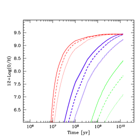
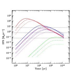
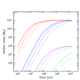
Figure 2: Predictions of O/H (left panel), SFR (middle panel), and $M_{\rm star}$ (right panel) vs. time in the MICE models. Models of two representative galaxies, $10^{8}$ $M_{\odot}$ and $10^{11}$ $M_{\odot}$, are coded by line type and color. The diffuse, compact, and hyper-dense cases are shown as dotted, dashed, and solid lines, respectively. Different galaxy masses are distinguished by color: green/dark violet for $10^{8}$ $M_{\odot}$, and blue/red for $10^{11}$ $M_{\odot}$ (SE/RE, respectively). In the middle panel, dotted horizontal lines show the four SFR regimes considered here: $\mbox{SFR}\leq 0.06$ $M_{\odot}$ yr^-1, $0.06<\mbox{SFR}\leq 0.6$ $M_{\odot}$ yr^-1, $0.6<\mbox{SFR}\leq 6$ $M_{\odot}$ yr^-1, and $\mbox{SFR}\geq 6$ $M_{\odot}$ yr^-1.

For a given galactic mass, $M_{\rm gal}$, RE galaxies evolve much more rapidly than SE galaxies. They accumulate metals and build a considerable fraction of their stellar mass in a shorter time ($\sim 10^{8}$ yr for $M_{\rm gal}=10^{11}$ $M_{\odot}$, and $\sim 10^{9}$ yr for $M_{\rm gal}=10^{8}$ $M_{\odot}$). Slowly-evolving disk-like galaxies of the same mass need much more time for metal production and to assemble stellar mass ($\sim 10^{9}$ yr and more than a Hubble time to produce the same stellar fraction, respectively). This signature of chemical downsizing, here closely related to mass downsizing, stems from the considerable fraction of the stellar mass in massive galaxies formed in less than 1 Gyr, while 50% or more of the stellar mass of less massive galaxies is still being created at the present time. This is because of the high efficiency of star formation of RE galaxies in their formation phase.

For a given galactic mass, SFR also peaks at earlier times for RE galaxies with respect to SE galaxies, as already found by Sandage (1986). Galaxies with denser molecular clouds (i.e., a more active SF mode) have a higher maximum value of the SFR with an earlier onset than galaxies with less dense clouds. Within either SE or RE galaxies, for a specific cloud density, more massive galaxies reach a higher SFR and at earlier times than less massive galaxies (because of their increased star-formation efficiency, see also Tosi & Diaz, 1985).

At a given molecular cloud gas density, $n_{\rm MC}$, more massive galaxies evolve more rapidly than less massive ones (e.g., downsizing). For the most massive galaxies, $M_{\rm gal}=10^{11}$ $M_{\odot}$, the final oxygen abundances are similar for the rapidly- and SE families, with slightly lower values for SE galaxies, even though these values are reached over different timescales. For the least massive galaxies with $M_{\rm gal}=10^{8}$$M_{\odot}$, SE and RE galaxies achieve different metallicities at the present epoch. Again, this is because of chemical downsizing, since less massive galaxies form stars less efficiently. Thus, although SE disk-like galaxies with $M_{\rm gal}=10^{8}$$M_{\odot}$ have the potential to reach the same metallicity of RE galaxies of the same mass, they will do so only on timescales much longer than a Hubble time. They also require more than a Hubble time to fully convert all their gas into stars.

Within each class (SE, RE), galaxies with the densest clouds evolve faster. These differences again result from the star formation efficiency which, in our models, depends also on the free-fall time of the molecular clouds.

The left panel of Fig. 2 shows the degeneracy between the track of the SE galaxy with $M_{\rm gal}=10^{11}$ $M_{\odot}$ and that of the RE galaxy with $M_{\rm gal}=10^{8}$ $M_{\odot}$. The scaling factors described in Sect. 3.3 conspire to make the behaviour of these two galaxies virtually identical in terms of metallicity evolution. However, the evolutionary timescales of the SFR and the stellar mass differ, suggesting that metallicity alone is not a good indicator of the evolutionary status of a galaxy. Specifically, a slowly evolving massive galaxy and a low-mass rapidly evolving galaxy will have similar metallicities.

Indeed, Fig. 2 also shows that for a given galactic mass, it is possible to achieve the same metal abundance (left panel) with different SFRs (middle) and different stellar masses (right). The galaxy can be less massive but, because of its active mode, more rapidly form stars, and thus accumulate more metals and stellar mass on shorter timescales. Alternatively it can be more massive and thus produce more of everything, but can also form stars and accumulate metals more slowly. The key aspect of our modeling is the evolutionary timescale which is parametrized either through the global properties of the galaxies, governed by how we have scaled our models (i.e., slow vs. rapid evolution), or through the density of the gas in the molecular clouds within the galaxies. Either way, shorter dynamical times drive more rapid evolution. We will discuss below how these effects can help explain the active vs. passive dichotomy, and consequently how we can better understand the behavior of low-metallicity starbursts, and their departure from the scaling relations.

In any case, the present-day abundances of our model galaxies are somewhat high. This is almost certainly due to the closed-box nature of our models and the lack of gas exchange with the environment. In fact, this is what led chemical evolution modelers to introduce both infall of metal poor gas and later also galactic winds powered by supernova explosions in order to reduce the predicted metal abundances and bring them to a better agreement with the observed ones (Matteucci & Tosi, 1985; Tosi, 1988; Pilyugin, 1993). Without galactic winds the products of stellar nucleosynthesis are always retained, and without infall of pristine gas they are never diluted. It is well known that gas accretion and expulsion can significantly alter the chemical abundances in galaxies (e.g., Matteucci & Tosi, 1985; Pilyugin, 1993; Marconi et al., 1994; Romano et al., 2006).

However, infall and/or outflow are not the only mechanisms that could vary the abundances. The absolute level of the abundance depends also on the combination of the adopted stellar yields and IMF. Magrini et al. (2010) have shown that the maximum variation of the abundance level in the disk of the spiral galaxy M 33 obtained by varying the parametrization of the IMF (and keeping fixed the stellar yields) is $\sim$0.6 dex, with the Chabrier IMF having the higher abundances. The impact of adopting different stellar yields, e.g., considering or not stellar rotation, could be $\sim$0.2 dex at solar metallicity (c.f., Romano et al., 2010). Thus, considering quadratically the two effects, the absolute abundance level could vary by up to $\sim$0.6 dex without invoking infall/outflow processes. In any case, the approach presented here should be considered as a first step toward better understanding the interplay of the three observables; future work will be aimed at comparing our current results with models having gas inflow and outflow and with different IMFs and stellar yields.

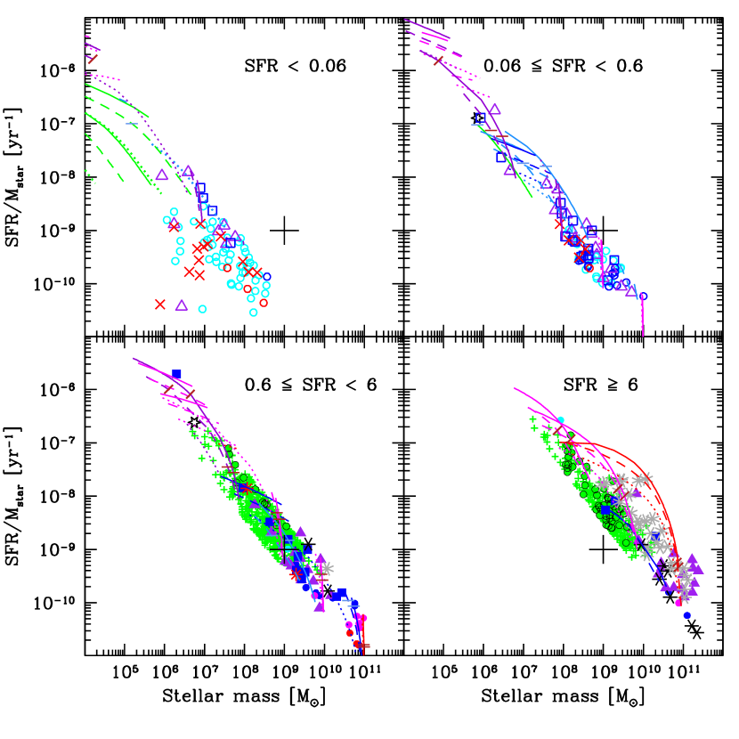
Figure 3: Specific SFR vs. stellar mass divided into four ranges of SFR: $\mbox{SFR}\leq 0.06$ $M_{\odot}$ yr^-1, $0.06<\mbox{SFR}\leq 0.6$ $M_{\odot}$ yr^-1, $0.6<\mbox{SFR}\leq 6$ $M_{\odot}$ yr^-1, $\mbox{SFR}\geq 6$ $M_{\odot}$ yr^-1. LVL (11HUGS) galaxies are shown as small open or filled circles (filled when SFR$\geq$0.6 $M_{\odot}$ yr^-1), with different colors corresponding to Hubble type $T$ as in Lee et al. (2009): $T\geq$ 8 cyan, $5\leq T<8$ blue, $3\leq T<5$ magenta, and $T<3$ red. Red $\times$ corresponds to the dIrr sample; BCDs are shown as (blue) squares (Fumagalli$+$Hunt samples) and (purple) triangles (Engelbracht); Green Peas are given by small (green) filled circles; LCGs by (green) $+$; LBGs at $z\sim 1$ (Shapley), $z\sim 2$ (Erb, Shapley) are shown as 6-pronged asterisks, and at $z\sim 3$ (Maiolino, Mannucci) as 8-pronged asterisks. 6-sided open stars show the two dwarf “prototypes”, SBS 0335$-$052 and I Zw 18. Solid symbols show those BCDs with SFR$\geq$0.6 $M_{\odot}$ yr^-1. Models are coded by line type and color as in Fig. 2. The corresponding colour codes for the stellar masses (SE/RE, respectively) are: green/dark violet for $10^{7}$, $10^{8}$ $M_{\odot}$, light blue/magenta for $10^{9}$, $10^{10}$ $M_{\odot}$, and blue/red for $10^{11}$ $M_{\odot}$. The evolution times are marked along the tracks: an inclined tick indicates 100 Myr (only for the RE galaxies), and a horizontal tick 1 Gyr. Time increases downward and to the right. The large $+$ sign is a fiducial point (sSFR = 10^-9 yr^-1, $M_{\rm star}$ = 10⁹ $M_{\odot}$) which guides the eye to the differences in the main loci of data points and models in the different panels.

4.2 The SFMS and the MZR

Here we compare the model results with the observed SFMS (sSFR vs $M_{\rm star}$ relation) and the MZR (mass-metallicity relation). We also show the models superimposed on the Fundamental Plane identified in Paper I. To better visualize the interplay among the observables, and isolate different regions of parameter space, we have divided the models and the data into two regimes of SFR: the “passive” one with SFR$<$0.6 $M_{\odot}$ yr^-1, and the “active” one with SFR$\geq$0.6 $M_{\odot}$ yr^-1. This threshold was defined in Paper I on the basis of the onset of deviations from the SFMS and the MZR; for our sample, these deviations become significant at all redshifts for SFR$\ga$0.6 $M_{\odot}$ yr^-1, roughly the equivalent of NGC 4826 (M 64, the Black-Eye Galaxy), 1.5 times M 33 or the “dwarf starburst” NGC 3077, or twice the SFR of M 31 (Dale et al., 2012; Verley et al., 2007; Meier et al., 2001; Tabatabaei & Berkhuijsen, 2010). We have further divided these two regimes into two sectors, in order to better separate and identify the progression from passive to active modes. In all of the following plots, we show models at times from 1 Myr to a Hubble time, as given in Fig. 2.

4.2.1 The main sequence of star formation

Figure 3 shows the SFMS with sSFR plotted against stellar mass. Galaxies characterized by a passive SF mode appear in the upper panels, while active galaxies are in the bottom ones. Models of RE and SE galaxies, with their mass “families” and three different MC density regimes, are also shown and divided into different SFR regimes. Evolution timescales are marked along the tracks: an inclined tick indicates 100 Myr (only for the RE galaxies), and a horizontal tick 1 Gyr. The $+$ marks an arbitrarily defined fiducial position in order to guide the eye to the displacements in the various panels as a function of SFR (see below).

The least massive most quiescent galaxies (see upper left panel) have very low sSFRs, and are modeled only by the very end points of SE galaxies. As SFR increases (upper right), galaxies are more massive and the data are well reproduced by SE models with either low masses and compact MCs (the “intermediate” SF mode), or higher masses and diffuse clouds (the passive mode). Data in the bottom left panel (the onset of the active SF mode), are well modeled by intermediate-mass SE or RE galaxies with dense or hyper-dense clouds, but also by the most massive SE galaxies (or RE galaxies) with diffuse clouds. As discussed in Sect. 3.3, both galaxy mass and cloud density contribute to SFR and evolutionary timescales.

The most extreme starbursts in the bottom right panel are reproduced only by RE galaxies and the most massive SE galaxies with hyper-dense and compact clouds. Moreover, such high SFRs are achieved by the most massive RE models and the most massive hyper-dense SE only up to an age of $\;\buildrel<\over{\sim}\;$200–500 Myr from the onset of the SF episode (see Fig. 2). Thus galaxies with these high SFRs are expected to be “young”, i.e., “captured” in a relatively early phase of their evolution. However, the RE models have assembled almost all their stellar mass (and metals) already at these early times, but the SE models will continue to build up their stellar and metal content for some time to come.

The $+$ in Fig. 3 represents a fiducial point (arbitrarily defined), with the aim of guiding the eye to the changes in loci among the panels. In the upper left panel, the galaxies fall below the fiducial by almost an order of magnitude in both axes; in the upper right and lower left, the galaxies (and models) are roughly coincident; in the last panel both galaxies and models fall above the fiducial by a factor of 5 or so in both sSFR and stellar mass. Many LCGs and Green Peas at $z\sim 0.3$, and some BCDs at $z\sim 0$, are coincident with the LBGs in the AMAZE and LSD samples at $z\sim 3$. These galaxies are modeled by systems in early stages of their evolution, and with high SFR. Hence, at least in this parameter space of SFR and $M_{\rm star}$, there are local galaxy populations which mimic the properties of galaxies at high redshift. They are distinguished by their relatively high SFR, perhaps resulting from a similar selection effect for both the low- and high-redshift samples.

4.2.2 The mass-metallicity relation

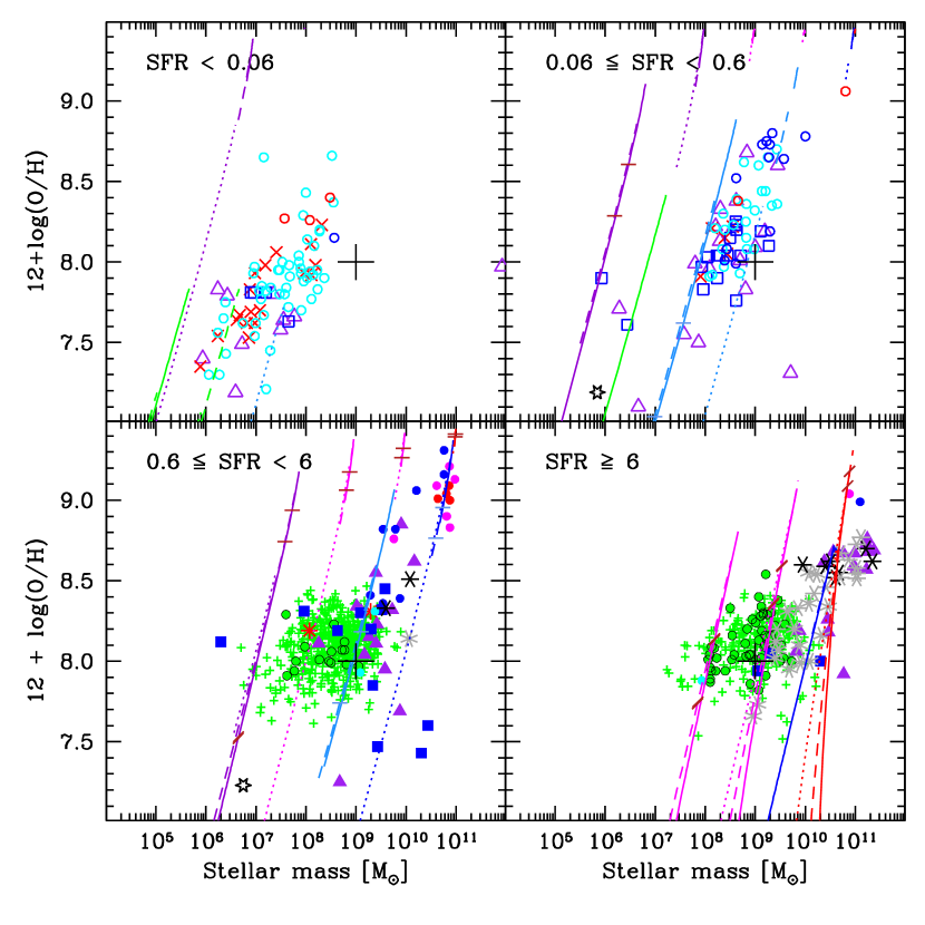
Figure 4: Nebular oxygen abundance vs. stellar mass $M_{\rm star}$ divided into regions of SFR. The four regimes we consider are: $\mbox{SFR}\leq 0.06$ $M_{\odot}$ yr^-1, $0.06<\mbox{SFR}\leq 0.6$ $M_{\odot}$ yr^-1, $0.6<\mbox{SFR}\leq 6$ $M_{\odot}$ yr^-1, $\mbox{SFR}\geq 6$ $M_{\odot}$ yr^-1. Symbols are as in Fig. 3. Models are coded by line type and color as in Fig. 3: diffuse as dotted lines, compact as dashed, and hyper-dense as solid lines. The corresponding colour codes for the stellar masses (SE/RE, respectively) are: green/dark violet for $10^{7}$, $10^{8}$ $M_{\odot}$, light blue/magenta for $10^{9}$, $10^{10}$ $M_{\odot}$, and blue/red for $10^{11}$ $M_{\odot}$. The evolution times are marked along the tracks: an inclined tick indicates 100 Myr (only for RE galaxies), and a horizontal tick 1 Gyr. Time increases upward and to the right. The large $+$ corresponds to a “fiducial” value of $M_{\rm star}$ = 10⁹ $M_{\odot}$, and 12$+\log$(O/H) = 8.0, intended to guide the eye to differences among the panels as in Fig. 3.

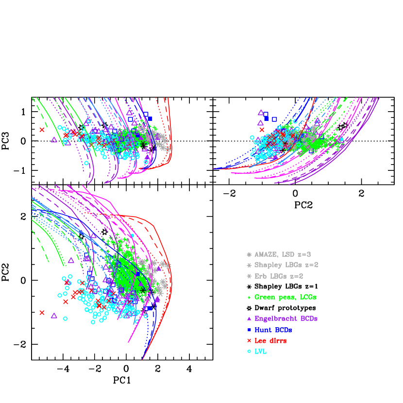
Figure 5: Different projections using the 3 PCs found by the PCA. Galaxies are coded as shown in the lower right (empty) panel. The top left and right panels show the orthogonal “edge-on” views of the plane; the bottom panel shows the plane face-on. $x_{1}\,=\,$12$+\log$(O/H)$-\langle$ 12$+\log$(O/H)$\rangle$, $x_{2}\,=\,\log(SFR)-\langle\log(SFR)\rangle$ ($M_{\odot}$ yr^-1), and $x_{3}\,=\,\log(M_{\rm star})-\langle\log(M_{\rm star})\rangle$ ($M_{\odot}$). $\langle$12$+\log$(O/H)$\rangle$ =  8.063; $\langle\log(SFR)\rangle$ =  -0.594; $\langle\log(M_{\rm star})\rangle$ = 8.476. PC1   =   0.12 $x_{1}$ + 0.75 $x_{2}$ + 0.65 $x_{3}$; PC2   =   -0.31 $x_{1}$ - 0.65 $x_{2}$ - 0.69 $x_{3}$; PC3   =   -0.94 $x_{1}$ - 0.11 $x_{2}$ + 0.31 $x_{3}$. The axes are expanded in the top panels to exaggerate the variations in PC3, relative to the much larger dynamic ranges in PC1 and PC2. MICE models are superimposed similarly to previous figures, but here there are no temporal tick marks. In all three panels, time increases downward.

The MZR is shown in Fig. 4, divided into four SFR regimes as in Fig. 3. Low-mass galaxies with relatively high metallicities (top left panel) are not well reproduced with our MICE models. This is probably because our SE models require more than a Hubble time to complete the stellar mass assembly and metal production with the available fuel. Ongoing accretion could help here, but it would also be necessary to shorten timescales in order to accelerate the gas consumption. As SFR increases (top right), intermediate-mass SE galaxies are able to well reproduce the data, either more massive models with diffuse clouds or less massive ones with compact or hyper-dense clouds.

Galaxies forming stars in the active mode (bottom left panel) are well reproduced by the more massive SE galaxies and the less massive RE galaxies. The most massive SE galaxy (10¹¹ $M_{\odot}$) with diffuse clouds is consistent with the most metal-rich observations, and also the most metal-poor ones. Interestingly, the latter appear to lie along the same evolutionary path as the former and may evolve into them. However, an active SF mode with compact or hyper-dense clouds is necessary to reproduce the observations at lower masses: either SE galaxies for masses $10^{8}-10^{9}$ $M_{\odot}$, or RE galaxies for lower masses.

Extreme starbursts (bottom right panel) require rapidly evolving models at young ages for such high SFRs; galaxies must be younger than $\;\buildrel<\over{\sim}\;$200-300 Myr (see Fig. 2). The main population of the galaxies in this panel can be reproduced only with the early phases of the evolutionary tracks of RE (starburst) galaxies. Only a single SE galaxy model, the most massive one with hyper-dense molecular clouds, appears in this panel. Below, we explore how the gas content of the models changes with SFR (and age) in order to better understand the evolutionary phase of these galaxies.

4.3 The fundamental plane of metallicity, SFR, and stellar mass

Our models have been rather successful at reproducing the observed trends in the SFMS and MZR. However, in Paper I, we introduced a Fundamental Plane (FP) which enabled an accurate (0.17 dex) determination of O/H given SFR and $M_{\rm star}$. Here we show that our models also well reproduce the FP, and occupy the same spread in parameter space as the observations.

Figure 5 shows the Fundamental Plane that emerged from the Principle Component Analysis (PCA) of Paper I. The two upper panels show the edge-on views of the plane, and the bottom panel the face-on one. Our models are superimposed on the data and are consistent with the loci of the data in all three projections. In all three plots, time increases downward.

5 Gas fractions and metal abundance

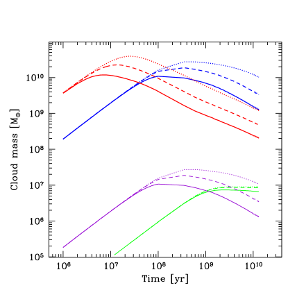
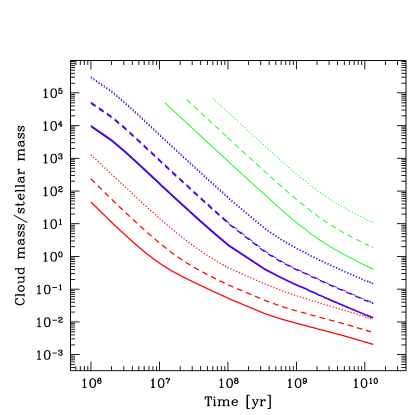
Figure 6: Predictions of H₂ mass (left panel) and ratio of H₂ to $M_{\rm star}$ (right panel) vs. time in the MICE models. As in Fig. 2, we show only models of two representative galaxies, $10^{8}$ $M_{\odot}$ (green/dark violet) and $10^{11}$ $M_{\odot}$ (blue/red), for the SE/RE types, respectively. The diffuse (dotted lines), compact (dashed), and hyper-dense cases (solid lines) are coded by line type. In these models, the cloud-formation efficiency and SFR efficiency both scale with cloud mass as: $M_{\rm MC}^{1/3}$.

Most previous interpretations of the shape of the MZR have relied on gas inflow and outflow, with the assumptions that outflowing gas is chemically enriched and that infalling gas is not (e.g., Tolstoy et al., 2009; Mannucci et al., 2010; Davé et al., 2012; Yates et al., 2012; Dayal et al., 2012). As already discussed, our MICE models are “closed-box”, and thus neglect the effects of gas inflow and outflow. Nevertheless, as we have shown in previous sections, the predictions of our models are in good agreement with the SFMS and the MZR through the active/passive dichotomy of SF modes and the resulting evolutionary timescales. Here we examine the MICE model predictions for the molecular gas mass fractions relative to stellar mass, and compare them with observations of local and high-$z$ samples with measured H₂ and stellar masses.

The time evolution of the H₂ content (“cloud” mass) and the cloud-to-stellar mass ratio is shown in Fig. 6. The right panel of this figure, as in Fig. 2, shows the degeneracy between the track of the SE galaxy with $M_{\rm gal}=10^{11}$ $M_{\odot}$ and that of the RE galaxy with $M_{\rm gal}=10^{8}$ $M_{\odot}$. The scaling factors conspire to make these two galaxies behave similarly in any quantity which is normalized (i.e., O/H, H₂/$M_{\rm star}$). However, as before, the different timescales for the different SF modes make the gas fraction relative to stars (and chemical abundance) non-unique tracers of evolution. A low-mass RE spheroid can achieve similar metallicity and gas mass fraction as a more slowly evolving, but more massive, SE galaxy. The gas fraction of the rapidly evolving spheroid will be higher than that of the more slowly evolving galaxy, as long as we observe the former at an earlier evolutionary phase than the latter.

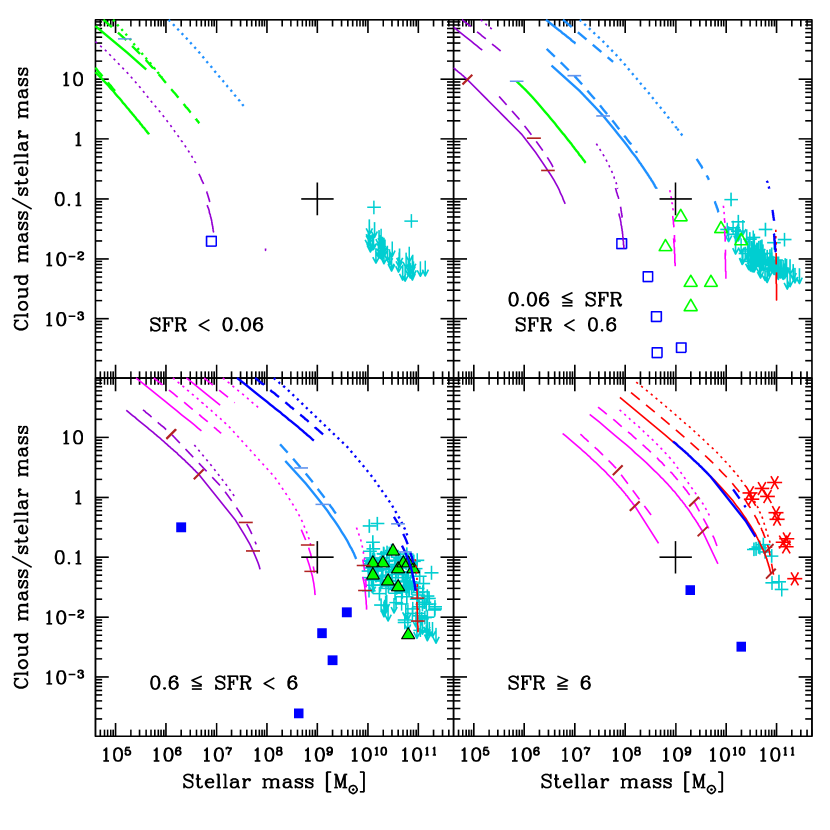
Figure 7: Ratio of molecular cloud mass and $M_{\rm star}$ vs. stellar mass $M_{\rm star}$ divided into regions of SFR. The four regimes we consider are: $\mbox{SFR}\leq 0.06$ $M_{\odot}$ yr^-1, $0.06<\mbox{SFR}\leq 0.6$ $M_{\odot}$ yr^-1, $0.6<\mbox{SFR}\leq 6$ $M_{\odot}$ yr^-1, $\mbox{SFR}\geq 6$ $M_{\odot}$ yr^-1. Squares (blue) correspond to the BCDs from Fumagalli et al. (2010), triangles (green) to the spiral galaxies from Leroy et al. (2008), and 6-pronged asterisks to the SMGs from Hainline et al. (2011). Turquoise $+$ and down-arrows indicate the COLDGASS molecular gas content from Saintonge et al. (2011a, b). Models are coded by line type and color as in Fig. 3. The evolution times are marked along the tracks: an inclined tick indicates 100 Myr (only for RE galaxies), and a horizontal tick 1 Gyr. Time increases downward and to the right. The large $+$ corresponds to a “fiducial” value of cloud mass/$M_{\rm star}$ of 0.1 and $M_{\rm star}$ = 10⁹ $M_{\odot}$, intended to guide the eye to differences among the panels.

In Fig. 7 we have plotted the ratio of molecular cloud to stellar mass vs. $M_{\rm star}$, separated into four panels of SFR as in previous figures. Also shown are several samples including the BCDs from Fumagalli et al. (2010) (also considered in the previous analyses), spiral galaxies from Leroy et al. (2008), galaxies from the COLDGASS survey by Saintonge et al. (2011a, b), and sub-millimetre galaxies (SMGs) at $z\sim 2-3$ from Hainline et al. (2011). Conversion factors $X_{\rm CO}$ to derive H₂ mass (“cloud mass” in Fig. 7) are given in the respective papers, and vary with galaxy type.

The main problem with comparing molecular content of metal-poor starbursts (lower left and lower right panels in Fig. 7) lies with the intrinsic difficulty of detecting molecules in the cool gas phase in a metal-poor ISM (e.g., Taylor et al., 1998; Barone et al., 2000; Leroy et al., 2005). Moreover, the conversion of CO intensities to H₂ mass at low metallicities is very uncertain (e.g., Bolatto et al., 2008; Leroy et al., 2009; Wolfire et al., 2010; Leroy et al., 2011). While Bolatto et al. (2008) find $X_{\rm CO}$ not to vary significantly with metal abundance in Local Group galaxies, at metallicities 12$+\log$(O/H)$\lower 2.15277pt\hbox{$\;\buildrel<\over{\sim}\;$}8.2$ there is evidence for $X_{\rm CO}$ factors of 10 to 20 times higher (Leroy et al., 2009, 2011). For the BCDs with CO observations in Fumagalli et al. (2010), we have used a conservative value, $X_{\rm CO}\,=\,4\times 10^{20}$ cm^-2 [K km s${}^{-1}]^{-1}$, (e.g., Bolatto et al., 2008); hence, the estimates of H₂ mass in the metal-poor BCDs shown in Fig. 7 could be highly underestimated (and in fact are outliers because of their low inferred cloud mass/stellar mass ratios).

The MICE model predictions of the ratio of molecular gas mass to stellar mass shown in Fig. 7 are in fairly good agreement with the observations, excepting the COLDGASS upper limits in the upper left panel with SFR$<$0.06 $M_{\odot}$ yr^-1. This consistency is perhaps surprising, given that our models are closed box, but strongly suggests that other parameters, such as dynamical timescales resulting from compact size and high density, play an important, if not primary, role in governing gas fractions.

Comparison with Figs. 3 and 4 indicate that the models that reproduce the scaling relations between SFR, stellar mass, and O/H in the upper panels are relatively gas poor. The upper left panel in Fig. 3 is not well reproduced by our models because the galaxies tend to be more massive than expected from the sSFR; this is perhaps propagating into Fig. 7 where galaxies are again too massive than would be predicted from their low SFR and low cloud mass fraction. The upper right panel is apparently occupied by either RE RE galaxies or more slowly evolving galaxies which, in any case, are at the end of their lifetimes, having already converted most of their gas into stars. As the SFR increases (lower left panel), gas content also increases, and for the most extreme case (lower right panel), the mass ratio of molecular clouds to stars is $\sim$1, during the time when the galaxies also satisfy the scaling relations between metallicity, stellar mass, and SFR. The data for SMGs are entirely consistent with the models, and in fact have observed gas-to-total mass fractions [clouds/(stars$+$clouds)] of 50% or more (Tacconi et al., 2006).

With our MICE models we are able to link the gas content and the SFR with the evolutionary timescales. The galaxies we call active are observed close to the peak of the SFR with a still high gas content, and are relatively chemically unevolved. During that phase of their evolution they are still gas-rich star-forming galaxies but will rapidly move toward the end of their SF phase. In fact, their evolution can be reproduced using chemical evolution models for RE (starburst) galaxies. On the other hand, passive galaxies are evolving at a very slow rate, so that their gas content and SFR will be relatively low during most of their lifetime.

Recently, Zahid et al. (2012) presented a sample of metal-rich low-mass galaxies, a galaxy population complementary to the metal-poor more massive starbursts discussed here. They interpreted the relatively high metallicities in their sample as due to the reduced gas content of the galaxies, such that the more metal-rich galaxies at a given stellar mass are more gas poor. In fact, the metal-rich low-mass galaxies studied by Zahid et al. (2012) would occupy the upper panels in Fig. 7. The interpretation of Zahid et al. (2012) is that at a given stellar mass, metal-rich galaxies have low gas fractions, and that the low gas fractions are largely responsible for the high gas-phase oxygen abundance observed. Instead, our models suggest that the highest metallicities at a given mass are not a consequence of the gas fraction, but that both gas fraction and metal abundance are consequences of evolutionary time scales, driven by the initial conditions in passive and active galaxies. Thus, our models also appear to verify the empirical conclusion reached by Zahid et al. (2012) that such galaxies are gas poor relative to their metal-poor counterparts at the same stellar mass.

6 Discussion

A significant fraction of galaxies in our sample deviates from the MZR and SFMS in similar ways, independently of redshift. These galaxies are apparently too massive for their metallicity, or alternatively, for their mass they are too metal-poor and have a SFR that is too high. The common characteristic of these galaxies, the low-metallicity starbursts, is the way they are selected from larger samples. Locally, metal-poor starbursts tend to come from objective-prism, emission line surveys; they are objects with strong H$\beta$, [Oiii$]\lambda$5007, or H$\alpha$ lines, and thus moderate dust extinction and high SFRs. At $z\lower 2.15277pt\hbox{$\;\buildrel>\over{\sim}\;$}1$, Lyman break selections, based on rest-frame UV colors, pick out star-forming galaxies with similar properties, namely relatively low dust extinction and relatively high SFRs (e.g., Shapley, 2011). Such galaxies also tend to be dominated by the most recent burst of star formation, with times from burst of a few tens of Myr to $\;\buildrel<\over{\sim}\;$1 Gyr (Shapley et al., 2005b; Haberzettl et al., 2012). At low redshift, this is a result of the selection of very high emission-line equivalent widths either in H$\alpha$ or in [Oiii] which implies that ionized gas makes a significant contribution to the total light (implying a young age). At high redshift, this is a function of the color selection for strongly star-forming galaxies that can be finely tuned to select galaxy populations at different redshifts. Hence, the low- and high-redshift LMSs, which deviate from the SFMS and the MZR in similar ways, have similar properties because of the way they are selected. In fact, together they form a Fundamental Plane of O/H, SFR, and $M_{\rm star}$, which is apparently independent of redshift.

The galaxies which deviate from the SFMS and MZR are well modeled by the active mode of star formation. The starbursts in the lower right panels of Figs. 3 and 4 are observed during the extreme starburst phase of their evolution which is rapid and intense, lasting up to $\;\buildrel<\over{\sim}\;$200-500 Myr. On the other hand, the galaxies which follow the general trends in the scaling relations form stars in the passive mode. The models suggest that they are observed during a more advanced long-lasting phase of their evolution, which endures most of their lifetime.

What are the drivers of the active and passive modes of star formation? There are two related aspects of our models which differentiate active and passive SF modes: their intrinsic characteristics in terms of size (RE vs. SE) and/or density of their star forming regions (diffuse, compact, and hyper-dense clouds), and their evolutionary age. The evolutionary age indicates the time from the last main episode of SF: for quiescent galaxies which have had an initial single main episode of SF, this might be comparable to a Hubble time, while for active galaxies it might be the time elapsed after the last major episode of SF. Thus when we refer to active galaxies as young objects, it means that they had their major episode of SF relatively recently, up to several hundreds of Myr ago.

The predictions of our models are in agreement with recent analyses of the structure of galaxies up to $z\sim 1$ along the SFMS (Wuyts et al., 2011). At all stellar masses and redshifts, they find that the largest disk-like galaxies lie along the SFMS; these would be the galaxies with the longest dynamical times. The star-bursting outliers are more centrally concentrated (compact) than the galaxies along the main sequence; these would have shorter dynamical times and thus be more rapidly evolving. Thus, our models correctly predict that compact RE active models reproduce the starburst outliers of the SFMS, and that SE galaxies, with their larger sizes and slower evolution, lie along it.

An active SF mode is more readily associated with mergers and interactions than a passive one; in fact, the initial conditions we attribute to active star formation may be induced by mergers and tidal compression. However, mergers are not the only way to foster a highly star-forming massive galaxy at $z\sim 2$ (e.g., Genzel et al., 2006). In fact, we hypothesize that the initial conditions for the active and passive modes of SF are governed by stochastic processes, which can occur even in isolation.

Although our MICE models reproduce the scaling relations of metallicity, stellar mass, and SFR rather nicely, they have limitations; as already discussed, the main one is they do not take into account either inflowing or outflowing gas. Other attempts to explain the MZR (and FMR) have been based on the transfer of gas, i.e., accretion of metal-poor gas and outflow of metal-enriched material (Mannucci et al., 2010; Yates et al., 2012; Davé et al., 2012; Dayal et al., 2012). Recent theoretical work, such as the “equilibrium approach” of Davé et al. (2012), consider stochastic rates of inflow and outflow that regulate SFR and the accumulation of stellar mass and metallicity. Such models are quite successful in approximating the shape of the MZR and its dependence on SFR, at least down to 12$+\log$(O/H)$\sim$8, SFR$\sim$1 $M_{\odot}$ yr^-1, and $M_{\rm star}$$\sim 10^{8.5}$ $M_{\odot}$ (Yates et al., 2012). It is not clear, though, whether they are consistent with the lower metallicities and higher SFRs in the deviant metal-poor starbursts.

Another limitation of our models is the way we approximate the onset of the molecular phase; the atomic gas must become molecular and form clouds before it can fuel star formation. Our models assume that molecular clouds form at a constant efficiency, with a dependence on atomic gas mass, and are disrupted by cloud-cloud collisions. More complex models take into account the self-shielding effect of dust on the UV interstellar radiation field (e.g., Krumholz et al., 2009; Krumholz & Gnedin, 2011). Although our models are successful in predicting the trends of the SFMS and the MZR, and observed gas fractions as in Fig. 7, they may be oversimplified. A more sophisticated treatment of the transition to molecular gas will be dealt with in a future paper (Schneider et al., in preparation).

Despite the limitations of the MICE models, they successfully predict the observed trends in scaling relations over a wide range of O/H, SFR, and $M_{\rm star}$. Their predictions are also in good agreement with observed molecular gas mass fractions and SFR. It is likely that some of the processes driving galaxy evolution are captured by our models, namely the formation of a dominant molecular phase, together with fast or slow evolutionary timescales depending on stochastic initial conditions. It is also likely that the physics behind galaxy evolution requires some gas exchange with the environment, and a regulation mechanism that drives an equilibrium between inflow and outflow (e.g., Davé et al., 2012). A combination of key features of both classes of models may be necessary to understand the mechanisms which drive evolution of galaxies in the early universe.

7 Conclusions

From a sample of $\sim 1100$ galaxies spanning a wide range of O/H, SFR, and $M_{\rm star}$, we have defined a class of low-metallicity starbursts which deviate from the SFMS and the MZR in the same way, independently of redshift. The sample taken as a whole (although excluding the galaxies with $M_{\rm star}$$\geq 3\times 10^{10}$ $M_{\odot}$) defines a Fundamental Plane whose orientation is defined primarily by SFR and $M_{\rm star}$, and whose thickness is governed by O/H. Our models show that this plane is populated by galaxies and by models with different modes of star formation: an active starburst mode that is more common at high redshift, and a more passive, quiescent mode that predominates in the local universe and that defines the main trends in the scaling relations. Summarizing the results shown in Figs. 3, 4, and 7, galaxies following the main trends in the SFMS and MZR form stars in the passive mode. They are well modeled by slowly evolving galaxies with only moderately dense molecular clouds (either “diffuse” or “compact” MCs) and a relatively low gas content. These galaxies spend most of their life in this quiescent, passive, evolutionary phase reaching asymptotically the conversion of their gas into stars in more than a Hubble time. We find that observations are consistent with the end-phases of the evolution of these galaxies predicted by our models. On the other hand, the galaxies which deviate from the SFMS and MZR form stars in the active mode, typical of gas-rich RE galaxies with masses from $10^{8}$ to $10^{11}$ $M_{\odot}$, or gas-rich SE galaxies with compact or hyper-dense clouds with masses of $\sim 10^{11}$ $M_{\odot}$. In the extreme cases of very high SFR, the evolutionary phase is short, suggesting that we are observing these galaxies just after the start of their most recent SF episode.

The existence of a Fundamental Plane and the success of our modeling of active/passive star formation implies that the SFMS and MZR do not really change with lookback time, but rather that the galaxy populations that define them change with redshift. The “evolution” in the scaling relations is a result of selecting those galaxies which are most common at a particular redshift. Equivalently, the scaling relations and the deviations from them result from different modes of star formation: an active starburst mode that is more common in the distant universe and a more passive quiescent one that dominates nearby.

References

- Aalto et al. (1995) Aalto, S., Booth, R. S., Black, J. H., & Johansson, L. E. B. 1995, A&A, 300, 369
- Atek et al. (2011) Atek, H., Siana, B., Scarlata, C., et al. 2011, ApJ, 743, 121
- Barone et al. (2000) Barone, L. T., Heithausen, A., Hüttemeister, S., Fritz, T., & Klein, U. 2000, MNRAS, 317, 649
- Bauer et al. (2011) Bauer, A. E., Conselice, C. J., Pérez-González, P. G., et al. 2011, MNRAS, 417, 289
- Bell & de Jong (2001) Bell, E. F., & de Jong, R. S. 2001, ApJ, 550, 212
- Boissier et al. (2001) Boissier, S., Boselli, A., Prantzos, N., & Gavazzi, G. 2001, MNRAS, 321, 733
- Bolatto et al. (2008) Bolatto, A. D., Leroy, A. K., Rosolowsky, E., Walter, F., & Blitz, L. 2008, ApJ, 686, 948
- Brinchmann et al. (2008) Brinchmann, J., Pettini, M., & Charlot, S. 2008, MNRAS, 385, 769
- Calura & Matteucci (2006) Calura, F., & Matteucci, F. 2006, ApJ, 652, 889
- Calura et al. (2009) Calura, F., Pipino, A., Chiappini, C., Matteucci, F., & Maiolino, R. 2009, A&A, 504, 373
- Cardamone et al. (2009) Cardamone, C., Schawinski, K., Sarzi, M., et al. 2009, MNRAS, 399, 1191
- Chabrier (2003) Chabrier, G. 2003, PASP, 115, 763
- Chanial et al. (2007) Chanial, P., Flores, H., Guiderdoni, B., et al. 2007, A&A, 462, 81
- Chieffi & Limongi (2004) Chieffi, A., Limongi, M. 2004 ApJ, 608, 405
- Dale et al. (2012) Dale, D. A., Aniano, G., Engelbracht, C. W., et al. 2012, ApJ, 745, 95
- Davé et al. (2012) Davé, R., Finlator, K., & Oppenheimer, B. D. 2012, MNRAS, 421, 98
- Dayal et al. (2012) Dayal, P., Ferrara, A., & Dunlop, J. S. 2012, arXiv:1202.4770
- De Lucia et al. (2006) De Lucia, G., Springel, V., White, S. D. M., Croton, D., & Kauffmann, G. 2006, MNRAS, 366, 499
- Engelbracht et al. (2008) Engelbracht, C. W., Rieke, G. H., Gordon, K. D., et al. 2008, ApJ, 678, 804
- Erb et al. (2006) Erb, D. K., Shapley, A. E., Pettini, M., et al. 2006, ApJ, 644, 813
- Erb et al. (2010) Erb, D. K., Pettini, M., Shapley, A. E., et al. 2010, ApJ, 719, 1168
- Ferrini et al. (1992) Ferrini, F., Matteucci, F., Pardi, C., & Penco, U. 1992, ApJ, 387, 138
- Ferrini et al. (1994) Ferrini, F., Mollá, M., Pardi, M. C., & Diaz, A. I. 1994, ApJ, 427, 745
- Fumagalli et al. (2010) Fumagalli, M., Krumholz, M. R., & Hunt, L. K. 2010, ApJ, 722, 919
- Galli & Ferrini (1989) Galli, D., & Ferrini, F. 1989, A&A, 218, 31
- Gavilán et al. (2005) Gavilán, M., Buell, J. F., Mollá, M. 2005, A&A, 432, 861
- Genzel et al. (2006) Genzel, R., Tacconi, L. J., Eisenhauer, F., et al. 2006, Nature, 442, 786
- Groves et al. (2008) Groves, B., Dopita, M. A., Sutherland, R. S., et al. 2008, ApJS, 176, 438
- Haberzettl et al. (2012) Haberzettl, L., Williger, G., Lehnert, M. D., Nesvadba, N., & Davies, L. 2012, ApJ, 745, 96
- Hainline et al. (2011) Hainline, L. J., Blain, A. W., Smail, I., et al. 2011, ApJ, 740, 96
- Hammer et al. (1997) Hammer, F., Flores, H., Lilly, S. J., et al. 1997, ApJ, 481, 49
- Hirashita & Hunt (2004) Hirashita, H., & Hunt, L. K. 2004, A&A, 421, 555
- Hoyos et al. (2005) Hoyos, C., Koo, D. C., Phillips, A. C., Willmer, C. N. A., & Guhathakurta, P. 2005, ApJL, 635, L21
- Hunt & Hirashita (2009) Hunt, L. K., & Hirashita, H. 2009, A&A, 507, 1327
- Hunt et al. (2012) Hunt, L., Magrini, L., Galli, D., Schneider, Bianchi, S., Maiolino, R., Romano, D., Tosi, M., Valiante, R. 2012, MNRAS, submitted (Paper I)
- Hunt et al. (2010) Hunt, L. K., Thuan, T. X., Izotov, Y. I., & Sauvage, M. 2010, ApJ, 712, 164
- Iwamoto et al. (1999) Iwamoto, K., Brachwitz, F., Nomoto, K., et al. 1999, ApJS, 125, 439
- Izotov et al. (2007) Izotov, Y. I., Thuan, T. X., & Stasińska, G. 2007, ApJ, 662, 15
- Izotov et al. (2011) Izotov, Y. I., Guseva, N. G., & Thuan, T. X. 2011, ApJ, 728, 161
- Jijina et al. (1999) Jijina, J., Myers, P. C., & Adams, F. C. 1999, ApJS, 125, 161
- Jun & Im (2008) Jun, H. D., & Im, M. 2008, ApJL, 678, L97
- Kennicutt (1998) Kennicutt, R. C., Jr. 1998, ARA&A, 36, 189
- Kennicutt et al. (2008) Kennicutt, R. C., Jr., Lee, J. C., Funes, S. J., José G., Sakai, S., & Akiyama, S. 2008, ApJS, 178, 247
- Kewley & Ellison (2008) Kewley, L. J., & Ellison, S. L. 2008, ApJ, 681, 1183
- Krumholz & Gnedin (2011) Krumholz, M. R., & Gnedin, N. Y. 2011, ApJ, 729, 36
- Krumholz et al. (2009) Krumholz, M. R., McKee, C. F., & Tumlinson, J. 2009, ApJ, 699, 850
- Krumholz & Tan (2007) Krumholz, M. R., & Tan, J. C. 2007, ApJ, 654, 304
- Krumholz & Thompson (2007) Krumholz, M. R., & Thompson, T. A. 2007, ApJ, 669, 289
- Lada et al. (1991) Lada, E. A., Bally, J., & Stark, A. A. 1991, ApJ, 368, 432
- Lara-López et al. (2010) Lara-López, M. A., Cepa, J., Bongiovanni, A., et al. 2010, A&A, 521, L53
- Larson (1981) Larson, R. B. 1981, MNRAS, 194, 809
- Lee et al. (2006) Lee, H., Skillman, E. D., Cannon, J. M., et al. 2006, ApJ, 647, 970
- Lee et al. (2009) Lee, J. C., Gil de Paz, A., Tremonti, C., et al. 2009, ApJ, 706, 599
- Leroy et al. (2009) Leroy, A. K., Bolatto, A., Bot, C., et al. 2009, ApJ, 702, 352
- Leroy et al. (2011) Leroy, A. K., Bolatto, A., Gordon, K., et al. 2011, ApJ, 737, 12
- Leroy et al. (2005) Leroy, A., Bolatto, A. D., Simon, J. D., & Blitz, L. 2005, ApJ, 625, 763
- Leroy et al. (2008) Leroy, A. K., Walter, F., Brinks, E., et al. 2008, AJ, 136, 2782
- Liu et al. (2008) Liu, X., Shapley, A. E., Coil, A. L., Brinchmann, J., & Ma, C.-P. 2008, ApJ, 678, 758
- Magrini et al. (2007) Magrini, L., Corbelli, E., & Galli, D. 2007, A&A, 470, 843
- Magrini et al. (2009) Magrini, L., Sestito, P., Randich, S., & Galli, D. 2009, A&A, 494, 95
- Magrini et al. (2010) Magrini, L., Stanghellini, L., Corbelli, E., Galli, D., & Villaver, E. 2010, A&A, 512, A63
- Maiolino et al. (2008) Maiolino, R., Nagao, T., Grazian, A., et al. 2008, A&A, 488, 463
- Mannucci et al. (2009) Mannucci, F., Cresci, G., Maiolino, R., et al. 2009, MNRAS, 398, 1915
- Mannucci et al. (2010) Mannucci, F., Cresci, G., Maiolino, R., Marconi, A., & Gnerucci, A. 2010, MNRAS, 408, 2115
- Marble et al. (2010) Marble, A. R., Engelbracht, C. W., van Zee, L., et al. 2010, ApJ, 715, 506
- Marconi et al. (1994) Marconi, G., Matteucci, F., & Tosi, M. 1994, MNRAS, 270, 35
- Matteucci (1994) Matteucci, F. 1994, A&A, 288, 57
- Matteucci & Tosi (1985) Matteucci, F., & Tosi, M. 1985, MNRAS, 217, 391
- Meier et al. (2001) Meier, D. S., Turner, J. L., & Beck, S. C. 2001, AJ, 122, 1770
- Melbourne et al. (2009) Melbourne, J., Bussman, R. S., Brand, K., et al. 2009, AJ, 137, 4854
- Mollá et al. (1996) Mollá, M., Ferrini, F., Diaz, A. I. 1996, ApJ, 466, 668
- Mollá et al. (1997) Mollá, M., Ferrini, F., Diaz, A. I. 1997, ApJ, 475, 519
- Mollá & Díaz (2005) Mollá, M., & Díaz, A. I. 2005, MNRAS, 358, 521
- Nelan et al. (2005) Nelan J.E., et al 2005, ApJ, 632, 137
- Noeske et al. (2007) Noeske, K. G., Weiner, B. J., Faber, S. M., et al. 2007, ApJL, 660, L43
- Peeples et al. (2009) Peeples, M. S., Pogge, R. W., & Stanek, K. Z. 2009, ApJ, 695, 259
- Pilyugin (1993) Pilyugin, L. S. 1993, A&A, 277, 42
- Pipino et al. (2009) Pipino, A., Silk, J., & Matteucci, F. 2009, MNRAS, 392, 475
- Reines et al. (2010) Reines, A. E., Nidever, D. L., Whelan, D. G., & Johnson, K. E. 2010, ApJ, 708, 26
- Renzini (2006) Renzini, A. 2006, ARA&A, 44, 141
- Romano et al. (2010) Romano, D., Karakas, A. I., Tosi, M., & Matteucci, F. 2010, A&A, 522, A32
- Romano et al. (2006) Romano, D., Tosi, M., & Matteucci, F. 2006, MNRAS, 365, 759
- Rosario et al. (2008) Rosario, D. J., Hoyos, C., Koo, D., & Phillips, A. 2008, IAU Symposium, 255, 397
- Rodighiero et al. (2011) Rodighiero, G., Daddi, E., Baronchelli, I., et al. 2011, ApJL, 739, L40
- Saintonge et al. (2011a) Saintonge, A., Kauffmann, G., Kramer, C., et al. 2011a, MNRAS, 415, 32 i
- Saintonge et al. (2011b) Saintonge, A., Kauffmann, G., Wang, J., et al. 2011b, MNRAS, 415, 61
- Salim et al. (2007) Salim, S., Rich, R. M., Charlot, S., et al. 2007, ApJS, 173, 267
- Salzer et al. (2009) Salzer, J. J., Williams, A. L., & Gronwall, C. 2009, ApJL, 695, L67
- Sandage (1986) Sandage, A. 1986, A&A, 161, 89
- Schiminovich et al. (2007) Schiminovich, D., Wyder, T. K., Martin, D. C., et al. 2007, ApJS, 173, 315
- Shapley (2011) Shapley, A. E. 2011, ARA&A, 49, 525
- Shapley et al. (2005a) Shapley, A. E., Coil, A. L., Ma, C.-P., & Bundy, K. 2005a, ApJ, 635, 1006
- Shapley et al. (2004) Shapley, A. E., Erb, D. K., Pettini, M., Steidel, C. C., & Adelberger, K. L. 2004, ApJ, 612, 108
- Shapley et al. (2005b) Shapley, A. E., Steidel, C. C., Erb, D. K., et al. 2005b, ApJ, 626, 698
- Simon et al. (2001) Simon, R., Jackson, J. M., Clemens, D. P., Bania, T. M., & Heyer, M. H. 2001, ApJ, 551, 747
- Smith & Hancock (2009) Smith, B. J., & Hancock, M. 2009, AJ, 138, 130
- Tabatabaei & Berkhuijsen (2010) Tabatabaei, F. S., & Berkhuijsen, E. M. 2010, A&A, 517, A77
- Tacconi et al. (2006) Tacconi, L. J., Neri, R., Chapman, S. C., et al. 2006, ApJ, 640, 228
- Tacconi et al. (2008) Tacconi, L. J., Genzel, R., Smail, I., et al. 2008, ApJ, 680, 246
- Talbot & Arnett (1973) Talbot, R. J., Jr., Arnett, W. D. 1973, ApJ, 186, 51
- Taylor et al. (1998) Taylor, C. L., Kobulnicky, H. A., & Skillman, E. D. 1998, AJ, 116, 2746
- Toft et al. (2009) Toft, S., Franx, M., van Dokkum, P., et al. 2009, ApJ, 705, 255
- Tolstoy et al. (2009) Tolstoy, E., Hill, V., & Tosi, M. 2009, ARA&A, 47, 371
- Tosi (1988) Tosi, M. 1988, A&A, 197, 33
- Tosi & Diaz (1985) Tosi, M., & Diaz, A. I. 1985, MNRAS, 217, 571
- Tremonti et al. (2004) Tremonti, C. A., Heckman, T. M., Kauffmann, G., et al. 2004, ApJ, 613, 898
- Verley et al. (2007) Verley, S., Hunt, L. K., Corbelli, E., & Giovanardi, C. 2007, A&A, 476, 1161
- Wolfire et al. (2010) Wolfire, M. G., Hollenbach, D., & McKee, C. F. 2010, ApJ, 716, 1191
- Wuyts et al. (2011) Wuyts, S., Förster Schreiber, N. M., van der Wel, A., et al. 2011, ApJ, 742, 96
- Yates et al. (2012) Yates, R. M., Kauffmann, G., & Guo, Q. 2012, MNRAS, 2572
- Zahid et al. (2012) Zahid, H. J., Bresolin, F., Kewley, L. J., Coil, A. L., Davé, R., ApJ, in press, arXiv:1203.0558