An Early & Comprehensive Millimeter and Centimeter Wave and X-ray Study of Supernova 2011dh: A Non-Equipartition Blastwave Expanding into A Massive Stellar Wind

Abstract

Only a handful of supernovae (SNe) have been studied in multi-wavelength from radio to X-rays, starting a few days after explosion. The early detection and classification of the nearby type IIb SN 2011dh/PTF 11eon in M51 provides a unique opportunity to conduct such observations. We present detailed data obtained at the youngest phase ever of a core-collapse supernova (days 3 to 12 after explosion) in the radio, millimeter and X-rays; when combined with optical data, this allows us to explore the early evolution of the SN blast wave and its surroundings. Our analysis shows that the expanding supernova shockwave does not exhibit equipartition ($\epsilon_{\rm e}/\epsilon_{\rm B}\sim 1000$), and is expanding into circumstellar material that is consistent with a density profile falling like $R^{-2}$. Within modeling uncertainties we find an average velocity of the fast parts of the ejecta of 15,000$\pm$1800 km/s, contrary to previous analysis. This velocity places SN 2011dh in an intermediate blast-wave regime between the previously defined compact and extended SN IIb subtypes. Our results highlight the importance of early ($\sim 1$ day) high-frequency observations of future events. Moreover, we show the importance of combined radio/X-ray observations for determining the microphysics ratio $\epsilon_{\rm e}/\epsilon_{\rm B}$.

1. Introduction

SN 2011dh in the nearby galaxy Messier 51 was discovered on UT 2011 May 31.893 by A. Riou; detected on June 01.19 UT by the Palomar Transient Factory (PTF, Law et al. 2009, Rau et al. 2009); and rapidly spectroscopically classified as a type IIb supernova (Arcavi et al. 2011a; 2011b).

The proximity of M51 (as in Arcavi et al. 2011b we assume a distance, $d=8.03\pm 0.77$ Mpc) motivated searches for the progenitor star. A putative massive star detected by the Hubble Space Telescope in pre-explosion images of M51 very close to the SN position was described by Maund et al. (2011) and Van Dyk et al. (2011). The interpretation of the progenitor is uncertain. Based on the rapid cooling of the expanding SN ejecta, Arcavi et al. (2011b) argue that the progenitor star must have a radius smaller than that of typical red supergiants or the supergiant progenitor of the well-studied Type IIb SN 1993J, see e.g., Weiler et al. (2007) (R$<10^{13}$ cm). In contrast, the astrometrically coincident star is a F8 supergiant. Reconciling these constraints means that the supergiant is either unrelated to the SN or was a companion of the (now erstwhile) progenitor star.

For core collapse supernovae the interaction of the blast wave with the circumstellar medium can generate detectable radio and X-ray emission. Additionally the fastest moving ejecta is related to the size of the progenitor (the more compact, the higher the velocity; Chevalier & Soderberg 2010). These two properties motivate early radio and X-ray observations. Thus, we began a program of centimeter and millimeter wave observations of SN 2011dh with EVLA and CARMA respectively. We initiated X-ray observations with the Swift Observatory. Following the end of our early monitoring a long-term program at EVLA was launched by A. Soderberg and collaborators. Their results are reported in a recent paper by Krauss et al. (2012).

Soderberg et al. (2012) analyzed the Swift X-ray and two epochs (day 4 and day 17) of radio observations of SN 2011dh, and found an expansion speed of $\approx 0.1c$ and a mass-loss rate of $6\times 10^{-5}\,M_{\odot}\,{\rm yr}^{-1}$. With these inferences they concluded that SN 2011dh is probably a type cIIb SN, namely a SN that originated from a compact progenitor star as opposed to one that originated from an extended progenitor star (eIIb); see Chevalier & Soderberg (2010) and references therein for explanation of these proposed sub-types. A similar result was found by Krauss et al. (2012).

Here we present a full set of centimeter and millimeter wave observations (from day 3 to day 12 after explosion) as well as an analysis of the Swift and Chandra X-ray observations of SN 2011dh. To our knowledge, these represent the most comprehensive (essentially daily) set of pan radio (5 GHz to 100 GHz) observations obtained at early times of a core collapse supernova. As a result we are able to probe the circumstellar matter at smaller radii (wherein one can expect to find deviations from homologous flows) and in principle directly infer the density of circumstellar matter.

The paper is organized as follows. The millimeter (CARMA) and centimeter (EVLA) observations are summarized in §2. In §3 we carry out a standard analysis for the radio observations assuming a synchrotron self-absorbed model. We then summarize the X-ray observations (§4) and present a combined radio+X-ray analysis (which incorporates inverse Compton scattering of optical photons to the X-ray band) in §5. We present our conclusions as well as review the returns obtained from early millimeter wave observations of core collapse supernovae (§6). Such a review is timely given the imminent operation of the Atacama Large Millimeter Array (ALMA).

2. CARMA and EVLA observations

Starting June 4, 2011, observations were undertaken with CARMA, centered on either 107 GHz or 93 GHz with an 8 GHz bandwidth in the D array configuration. For flux calibration we used either Uranus (whose flux was bootstrapped from observations of 3C345) or Mars. The compact source J1153+495 was used as a phase calibrator. The CARMA data were reduced using the MIRIAD reduction software. The log of observations can be found in Table 1 and a montage of CARMA detections is shown in Figure 1.

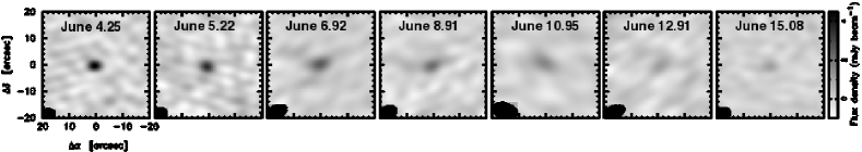
Figure 1.— CARMA image cutouts of SN 2011dh in the 3-mm band. The source at the center is SN 2011dh. The image cutouts are 40” on a side centered around SN 2011dh’s most precise position, based on our EVLA observations, at Right Ascension=13:30:05.104 and Declination =47:10:10.915 (J2000.0). The positional error is +/-0.01 arcsec in each axis (see text).

Observations with the EVLA were undertaken in the framework of our program “PTF Transients in the Local Universe” (PI: Kasliwal) as well as a ToO program to observe Type II Supernovae (PI: C. Stockdale). The array configuration was A. 3C286 served as the flux calibrator. We used the AIPS software to reduce the EVLA data. The first EVLA detection of the SN was in both the K (22.46 GHz) and Q (43.46 GHz) bands at fluxes of 2.6 mJy and 6.95 mJy, respectively. The log of the observations can be found in Table 1.

Table 1Summary of early radio observations of SN 2011dh

Day	Frequency	Flux
	[GHz]	[mJy]
4.21	4.8	$\leq 0.17$
4.21	7.4	0.203 $\pm$ 0.036 $\pm$ 0.01
4.25	22.5	2.6 $\pm$ 0.07 $\pm$ 0.26
4.23	43.2	6.95 $\pm$ 0.17 $\pm$ 0.7
4.08	107	4.55 $\pm$ 0.33 $\pm$ 0.46
4.08	230	$\leq 3$
5.01	8.5	0.455 $\pm$ 0.046 $\pm$ 0.023
5.12	22.5	3.95 $\pm$ 0.07 $\pm$ 0.4
5.10	43.2	6.47 $\pm$ 0.14 $\pm$ 0.65
5.22	107	3.66 $\pm$ 0.35 $\pm$ 0.36
6.92	93	2.52 $\pm$ 0.27 $\pm$ 0.25
7.12	8.5	1.06 $\pm$ 0.03 $\pm$ 0.053
7.20	43.2	6.42 $\pm$ 0.17 $\pm$ 0.64
7.22	22.5	6.89 $\pm$ 0.06 $\pm$ 0.69
8.91	93	1.84 $\pm$ 0.31 $\pm$ 0.18
9.02	22.5	7.46 $\pm$ 0.04 $\pm$ 0.75
9.02	8.5	1.58 $\pm$ 0.03 $\pm$ 0.079
9.06	5.0	0.42 $\pm$ 0.03 $\pm$ 0.021
9.12	33.6	7.49 $\pm$ 0.06 $\pm$ 0.75
10.95	93	1.61 $\pm$ 0.30 $\pm$ 0.16
11.01	43.2	3.19 $\pm$ 0.15 $\pm$ 0.32
11.03	22.5	8.17 $\pm$ 0.05 $\pm$ 0.82
11.98	8.5	3.15 $\pm$ 0.06 $\pm$ 0.158
12.02	5.0	1.22 $\pm$ 0.03 $\pm$ 0.061
12.91	93	1.06 $\pm$ 0.31 $\pm$ 0.106
15.08	93	1.05 $\pm$ 0.17 $\pm$ 0.105

Notes - Day is given in UT days in June 2011. The errors presented in the table represent the rms error from each image and a systematic calibration error ($5\%$ for $\nu<20$ GHz and $10\%$ for $\nu>20$ GHz) that should be combined in quadrature.

3. Standard Synchrotron Analysis

The radio emission arises from relativistic particles, which are accelerated at the shock, gyrating in magnetic fields, generated in the post-shock gas (Chevlaier 1982; Chevalier 1998; Weiler et al. 2002). A large body of work confirms that (for most supernovae) the early radio emission can be described by a synchrotron self-absorption (SSA) model (Chevalier 1998). While internal free-free absorption might also be present at early times, the lack of a steeper spectrum at the optically thick part of the spectrum suggests that SSA is dominant (see also Appendix 1). Hence, throughout this paper we adopt Chevalier (1998) SSA model.

Assuming a simple power law for the energy of the relativistic particles, the synchrotron emission for a self-absorbed source can be described by

$$S_{\nu}\propto\frac{\pi R^{2}}{D^{2}}B^{-1/2}\nu^{5/2}$$ (1)

for frequency, $\nu$ below $\nu_{a}$, where $\nu_{a}$ is the frequency at which the optical depth from synchrotron self-absorption is unity, and

$$S_{\nu}\propto\frac{4\pi fR^{3}}{3D^{2}}N_{0}B^{(p+1)/2}\nu^{-(p-1)/2},$$ (2)

for frequencies above $\nu_{a}$. Here, $B$ is the the strength of the magnetic field, $R$ is the radius of the blast-wave, $D$ is the distance from the observer to the supernova, $f$ is the volume fraction of the radio emitting region, and the energy spectrum of the relativistic particles is given by a power law, $N(E)=N_{0}E^{-p}$.

The SSA model does not attempt to predict the absolute or even the relative fraction of the two key components, the energy in relativistic electrons and the strength of the magnetic field. However, the minimum total energy will be achieved at equipartition, i.e., when the energy in the relativistic electrons is equal to that of the magnetic fields or $f_{\rm eB}=1$ (see Readhead 1994). Here $f_{\rm eB}$ is the ratio of the energy in relativistic electrons to that of the magnetic fields.

The measurement of the single-epoch SSA spectrum (both the optically thick and the optically thin parts) can be inverted to yield the radius and the magnetic field at that epoch (Chevalier 1998). For $p=3$ (which is the relevant case here; see §3.1):

$$R_{p} = 8.8\times 10^{15}f_{\rm eB}^{-1/19}\left(\frac{f}{0.5}\right)^{-1/19}\left(\frac{S_{p}}{\rm Jy}\right)^{9/19}\left(\frac{D}{\rm Mpc}\right)^{18/19}$$ (3)

$$\left(\frac{\nu_{p}}{\rm 5\,GHz}\right)^{-1}{\rm cm}$$

and

$$B_{p} = 0.58f_{\rm eB}^{-4/19}\left(\frac{f}{0.5}\right)^{-4/19}\left(\frac{S_{p}}{\rm Jy}\right)^{-2/19}\left(\frac{D}{\rm Mpc}\right)^{-4/19}$$ (4)

$$\left(\frac{\nu_{p}}{\rm 5\,GHz}\right){\rm G}.$$

Here, $S_{p}$ is the peak flux, and $\nu_{p}$ is the peak frequency. We assume $f=0.5$ (see Chevalier & Fransson 2006).

Equations 1 and 2 are adequate to describe the broad-band spectrum at any given epoch, as long as the emission is SSA. The dynamics of the supernova shell (which in turn depend on the velocity profile of the blast wave and the radial density distribution of the circumstellar medium) determine $R$ and $\nu_{a}$. These dependencies are generalized by allowing for power-law variations in key quantities (Weiler et al. 2002) and leading to the following equations:

$$S=K1\left(\frac{\nu}{{\rm 5\,GHz}}\right)^{\alpha}\left(\frac{t-t_{0}}{\rm 1\,day}\right)^{\beta}\left(\frac{1-e^{-\tau_{SSA}}}{\tau_{SSA}}\right),$$ (5)

where the absorption expression describes an internal absorption by material mixed with the emitting component and assumes planar geometry. The SSA optical depth is described by

$$\tau_{SSA}=K5\left(\frac{\nu}{\rm 5\,GHz}\right)^{\alpha-2.5}\left(\frac{t-t_{0}}{\rm 1\,day}\right)^{\delta^{{}^{\prime\prime}}},$$ (6)

where both $K1$ and $K5$ are proportionality constants that can be determined by fitting the data, and $\delta^{{}^{\prime\prime}}$ describes the time dependence of the optical depth.

3.1. Blast-wave physical parameters at single epochs

We analyze observations from the first five epochs: 2011 June 4, 5, 7, 9, and 11. During the first four epochs, data were obtained within a span of $\approx 4$ hours and thus are considered to be nearly simultaneous such that we assigned a central average time to all flux densities of a given epoch. We note that the last C-, and X-band observation were made on June 12 rather than on June 11 and therefore we obtain the C-, and X-band fluxes for June 11 by interpolation. For each epoch we fit the EVLA-CARMA spectrum to the SSA model characterized by $p$, $S_{p}$ and $\nu_{p}$ (Equations 1 and 2). We assume equipartition. For each epoch, the SSA model is well fitted by the data. The electron energy index, $p$, averaged over the five epochs we analyze is $p=3.00\pm 0.18$. Next, substituting our fitted parameters into Equations 3 and 4 we derive the magnetic field ($B)$ and radius ($R$) at each of our five epochs.

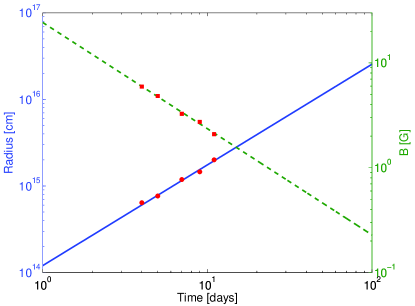
Figure 2.— The blast-wave radius (red circles) and magnetic field (red squares) estimates at 5 epochs. We assume an explosion date of May 31.5, 2011. Relative to this explosion date the epochs are [3.7, 4.6, 6.6, 8.5, 10.5] days. The corresponding values are: ${\rm R}\approx[0.64,0.77,1.19,1.46,2.01]\times 10^{15}{\rm cm}$ and ${\rm B}\approx[5.9,4.8,3.3,2.7,2.1]$G. Given the uncertainty in the peak fluxes, peak frequencies and $p$, we estimate the radius and magnetic field uncertainties to be $11\%$ and $9\%$, respectively. The curves are power law fits with $R\propto t^{1.14\pm 0.24}$ (solid blue line) and $B\propto t^{-1\pm 0.12}$ (dashed green line).

As shown in Figure 2, the blast-wave radius, $R\propto t^{m}$ where $m=1.14\pm 0.24$ while the magnetic field is proportional to $t^{-1\pm 0.12}$. Theoretically, the value of $m$ depends on the density structure of the blast wave. In particular, once the blast-wave decelerates, $m=1-(1/\eta)$ where $\eta$ is the velocity power-law index of the blastwave ($R\propto v^{-\eta}$). $\eta$ can be described as a function of the progenitor star polytropic index, $n$, where $\eta=(n+1)/(0.19\times n)$. For red supergiants (convective stars) $1\leq n\leq 3/2$ leading to $8.7\leq\eta\leq 10$, while for blue supergiants and Wolf-Rayet (radiative) stars $n=3$ leading to $\eta=7$. Unfortunately, our data lack the precision to discriminate between these two possibilities. Since theoretically $m\leq 1$ we conclude that the mean velocity of the shock (computed as $R/t$ where $t$ is the time since explosion) is about 21,000 km s^-1.

Next we can place a lower limit on the total energy. In principle, in addition to the energy in the electrons and in the magnetic field some energy can be carried by protons. We cannot estimate the proton energy. Thus the lowest estimate of the energy is given by the equipartition analysis and excluding that carried by protons (ions):

$$E_{\rm min}=\frac{B_{p}^{2}R_{p}^{3}}{6}\left(1+f_{\rm eB}\right)f$$ (7)

This yields (assuming $f_{\rm eB}=1$ and $f=0.5$) $E_{\rm min}\approx[1.6,1.8,2.9,3.8,5.8]\times 10^{45}$ erg at epochs of June 4, 5, 7, 9, and 11, respectively.

3.2. Time-dependent solution

We now fit the data to a comprehensive multi-epoch SSA model (as described by Equations 5 and 6). The resulting fit parameters are $\alpha=-1.15$, $\beta=-0.96$, $K1=453.43$, $K5=1.9772\times 10^{5}$, and $\delta^{{}^{\prime\prime}}=-3.42$. This implies an electron power law distribution with $p\approx 3$ and $R\propto t^{0.94}$ which is consistent with what we found in the single epoch analysis we performed above.

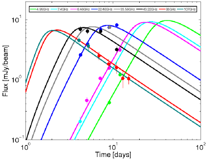
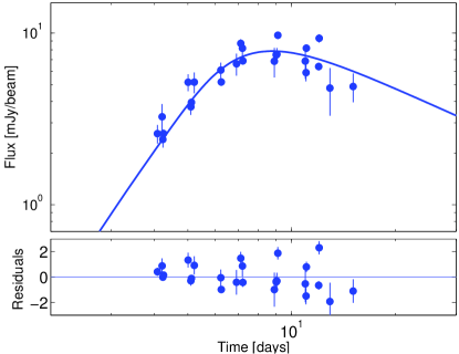
Figure 3.— Radio emission as a function of time. In the upper panel the result of the time-dependent fit (solid curves) is presented separately for each of the following frequencies $\nu=[107,93,43.22,33.56,22.46,8.46,7.4,4.95]$ GHz from left to right, respectively. In the lower panel the time-dependent fit and its residuals for a frequency of $\nu=22.46$ GHz is shown. The measurements presented in the lower panel were shifted to the latter frequency, assuming the fit parameters from §3.2.

Assuming the CSM was formed by a constant wind mass-loss, the CSM density structure will have the form $\rho_{\rm CSM}\propto r^{-2}$. We next calculate the electron number density which is given by $n_{e}=f_{\rm eB}\frac{(p-2)}{(p-1)}\frac{B^{2}}{8\pi\gamma_{m}m_{e}c^{2}}$, where $\gamma_{m}$ is the minimum electron lorentz factor (Soderberg et al. 2006). The resulting electron density is $n_{e}\approx 1.6-2.5\times 10^{5}\left(\frac{R}{10^{15}~{}{\rm cm}}\right)^{-2}{\rm cm}^{-3}$. In order to estimate the mass loss rate of the progenitor via wind prior to the explosion, $\dot{{\rm M}}=4\pi R^{2}n_{e}m_{p}v_{w}$, an assumption about the wind velocity, $v_{w}$, has to be made. Following Chevalier & Fransson (2006), instead of assuming a wind velocity we will scale the mass loss rate by it and define a new parameter, $A={\dot{M}}/{4\pi v_{w}}$. In the case of SN 2011dh, $A\approx 5\times 10^{11}$ g cm^-1, which is a factor of $3$ smaller than the value derived by Soderberg et al. (2011) and Krauss et al. (2012). This value of $A$ corresponds to a mass-loss rate of $10^{-7}\times(v_{w}/10~{}{\rm km~{}s^{-1}})$ M_⊙ yr^-1, consistent with a broad range of massive progenitor stars, from red supergiants to compact Wolf-Rayet stars.

4. X-ray Observations

SN 2011dh was observed with the Swift X-ray telescope (XRT; Burrows et al. 2003) in a series of observations beginning on 3.5 June 2011. We analyzed all observations taken through 23 June 2011 using the pipeline software of the UK Swift Science Data Centre at the University of Leicester, UK SSDC hereafter (Evans et al. 2007). To generate the X-ray light curve (see Figure 4), we fix the source position at the known location of the SN and extract a light curve with half-day binning (43.2 ksec per time bin) using an aperture of 35.4″. For background subtraction, we determine the time-average count rate in this identical aperture, $1.29\pm 0.14$ cts ks^-1 (0.3–10 keV), from pre-SN 2011dh Swift data.

The SN X-ray emission appears to fade rapidly at early times, so we split the observations in two for purposes of X-ray spectral analysis, fitting data from the first three time bins separately from the rest. The data are then fit to X-ray spectral models in XSPEC v 12.7.0 (Arnaud 1996), using a common Hydrogen column density ($N_{\rm H}$) across the full duration of the Swift observations and allowing the power-law photon ($\Gamma$) index and time-average flux to vary between the two data-sets. The resulting fit yields the following spectral parameters, where uncertainties here and below are quoted at 90%-confidence: $\mbox{$N_{\rm H}$}=1.1^{+1.3}_{-1.1}\times 10^{21}$ ${\rm cm}^{-2}$; $\Gamma_{1}=1.1\pm 0.4$; and $\Gamma_{2}=1.9^{+0.3}_{-0.4}$. The results suggests a softening of the X-ray emission over the course of the Swift observations but note that the photon index overlaps for $\Gamma=1.5$ at the 90%-confidence intervals.

Prior to analyzing the resulting X-ray flux light-curve (Fig. 4), we incorporate Chandra X-ray flux measurements from Pooley (2011) and Soderberg et al. (2011); these are converted to our chosen 0.3–10 keV bandpass using the authors’ chosen spectral models and the WebPIMMS tool. Analyzing the resulting X-ray light-curve, we find that it may be adequately characterized (in a $\chi^{2}$ sense) as a monotonic power-law decay emission. The single power-law temporal decay index is $\alpha_{X}=-1.2\pm 0.2$ over the interval of Swift and Chandra observations. The Chandra data confirm the absence of significant contaminating source emission within the Swift XRT aperture (Pooley et al. 2011; Soderberg et al. 2011).

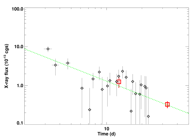
Figure 4.— X-ray light-curve of SN 2011dh (0.3–10 keV) as determined from Swift XRT observations (black diamonds) and the high-level analysis software at the UK Swift Science Data Centre (Evans et al. 2007). Error bars are $1\sigma$. Data have been binned to half-day intervals, with bins having less than 5% coverage dropped from analysis, and converted from counts to flux using the results of our X-ray spectral fits. The two red squares are Chandra measurements converted to (0.3–10 keV) band. A fit to the temporal decay is indicated as a single power-law decay (dotted green line). Counts-to-flux conversion factors (Swift observations) for the two spectral epochs (the first 3 bins and the rest of the bins) are $c_{1,a}=8.3\times 10^{-11}$ erg ${\rm cm}^{-2}$ s^-1 ct^-1 and $c_{2,a}=5.3\times 10^{-11}$ erg ${\rm cm}^{-2}$ s^-1 ct^-1, respectively, with respect to 0.3–10 keV absorbed flux, and $c_{1}=8.8\times 10^{-11}$ erg ${\rm cm}^{-2}$ s^-1 ct^-1 and $c_{2}=6.7\times 10^{-11}$ erg ${\rm cm}^{-2}$ s^-1 ct^-1, respectively, for 0.3–10 keV unabsorbed flux. The latter are the counts-to-flux conversion factors we use to generate the X-ray flux light-curve for SN 2011dh.

5. Combined Radio-X-ray-optical analysis

The X-ray photon index is 1.1 (early times) and 1.9 (late times). The high frequency radio spectral index is $-1$ which corresponds to a photon index of $2$. The X-ray emission is elevated by a factor of 50 relative to extrapolation of the SSA spectrum. Thus we conclude that the X-ray emission is not a result of synchrotron emission. Moreover, as already shown by Soderberg et al. (2012), thermal free-free X-ray emission is ruled out. Another explanation for the X-ray emission is that it arises from inverse Compton (IC) scattering of optical photons.

Assuming that the X-ray emission arises from IC, the SSA and IC formulation of Katz (2011) can be used to infer $R$ and $B$. For $p=3$

$$R\propto D\left(r_{\rm SIC}F_{t}\right)^{1/10}\left(S_{\nu,abs}\right)^{2/5}\left(\nu\right)^{-1}$$ (8)

$$B = 0.48\left(\frac{r_{\rm SIC}F_{t}}{10^{-12}{\rm erg~{}cm}^{-2}{\rm sec}^{-1}}\right)^{2/5}\left(\frac{S_{\nu,abs}}{{\rm mJy}}\right)^{-2/5}$$ (9)

$$\left(\frac{\nu}{10~{}{\rm GHz}}\right)~{}{\rm G},$$

where $r_{\rm SIC}=\nu S_{\nu,syn}/(\nu S_{\nu,IC})$, $S_{\nu,IC}$ is the IC flux, $S_{\nu,syn}$ is the synchrotron flux, $S_{\nu,abs}$ is the SSA flux, and $F_{t}$ is the optical flux.

Applying the Katz (2011) equations to the optical (Arcavi et al. 2011b), X-ray and radio measurements on June 7, 9 and 11 yields $B\approx[0.77,0.68,0.48]\,$G. The estimated error (obtained from application of the rule of error propagations) is $\approx 15\%$. These values of $B$ are $\approx 4.2$ smaller than the corresponding estimates obtained from an equipartition analysis (§3.1). Nominally, by using equation 4 again, $f_{\rm eB}\approx 500$ to 1700 with $10^{3}$ as a reasonable mean (which we adopt). However, as can be seen from Equation 3 this only results in a 30% decrease in the value of $R$, relative to that obtained from equipartition analysis (§3.1). Thus, the mean velocity is $R/t\approx 1.5\times 10^{9}\,$cm s^-1. The electron density is now higher by a factor of $\sim 50$ and therefore the mass-loss rate is higher by a factor of $\sim 20$ (for a fixed wind velocity).

6. Conclusions & Ramifications

In this paper we present the earliest millimeter- and centimeter-wave monitoring observations of the Type IIb supernova SN 2011dh in the galaxy M51, between four days and $12$ days after the event. Using the wide frequency coverage of the EVLA (4 to 43 GHz) and CARMA (100 GHz) we measure the key parameters of the synchrotron self-absorbed spectrum. The radio observations were accompanied by extensive X-ray observations by Swift. The X-ray emission, argued to be inverse Compton scattering of the SN optical photons by the relativistic electrons that produced the radio emission, combined with the radio observations, allow us to relax the equipartition assumption and track the radius and circumstellar density.

We infer a mean velocity of $R/t\approx 1.5\times 10^{9}\,$cm s^-1, for the SN shockwave, with an uncertainty entirely dominated by the limitations of the theoretical framework. Within the framework of the model the velocity is 1.32 to 1.68 $\times 10^{9}\,$cm s^-1. This value range is larger than the $\sim 10^{9}\,$cm s^-1 expected for an extended progenitor (red supergiant) but smaller than the $\sim 3\times 10^{9}\,$cm s^-1 expected for a compact progenitor. This may have important implications for the evolution leading to the formation of the progenitors of SNe IIb: if SNe IIb are split into two distinct, well-separated classes, that would suggest they may arise from two different evolutionary scenarios. On the other hand, if additional intermediate objects are found , that may suggest a continuum of objects between eIIb and cIIb, a single progenitor class may be favored.

We use the joint SSA+IC model analysis to infer the evolution of radius with time, $R\propto t^{m}$. We find $m=1.14\pm 0.24$. The error bars are too large to directly constrain the physical nature of the envelope of the exploding star (radiative versus convective). Assuming no additional systematics the combination of the early measurements with observations over several months may provide the means to determine the deceleration phase of the shock-wave in a more precise way and indirectly may shed more light on the density profile of the outer layers of the progenitor.

Soderberg et al. (2012) infer a much higher shock-wave velocity, $3\times 10^{9}$ cm s^-1, when assuming equipartition. As noted in §1 their analysis primarily rested on the X-ray data and optical data (since the radio data was quite sparse, day 4 and day 17). The limitations naturally propagate to the robustness of their inferences. This caveat notwithstanding, these authors find $f_{\rm eB}\equiv 30$, a factor of $\sim 30$ lower than the value we find, suggesting a shockwave velocity of $2.5\times 10^{9}$ cm s^-1. At least within the framework of the SSA+IC model we believe that our inference is more robust, thanks to our comprehensive radio and X-ray data sets. Moreover, as mentioned above, there is a factor of $3$ difference between the derived equipartition mass-loss rate value in our analysis compared to Soderberg et al. (2012) The origin of this difference is in the way this value is calculated and in the assumptions made. While Soderberg et al. (2012) assume $\epsilon_{e}=0.1$ we do not make such an assumption. Our measurements suggest $\epsilon\sim 0.3$ which accounts for the different mass-loss rate values.

Another set of comprehensive radio data was presented by Krauss et al. (2012) for days $>20$ after explosion. In their analysis they assumed equipartition only and found an average velocity of $\approx 25000$ km/s. Furthermore, assuming $\epsilon_{e}=0.1$, they found a mass-loss rate $3.5$ times greater than what we find. In view of these differences we analysed the data presented in Krauss et al. (2012) in the same manner that we analysed the early data set we present above. Our analysis suggests an average shockwave velocity of $18,500\pm 2000$ km/s at later times. Our derived lower velocity can be explained by a few factors. First, our fitting method allows the electron energy power-law index, $p$, to vary. We find an average value of $p=2.8$, while Krauss et al. (2012) keep the power-law index constant at $p=3$. This leads to slightly different values of the peak flux and frequency which in turn leads to a lower value of the velocity. Another factor that contributes to the difference between Krauss et al. (2012) and our velocity value is the different coefficient used in Equation $3$. While we are using the coefficient from Chevalier et al. (1998), Krauss et al. (2012) use a coefficient which is larger by $20\%$. When using Krauss et al. (2012) values for the peak frequencies and fluxes in Equation $3$ using our coefficient, we find an average shockwave velocity of $21,000$ km/s which is consistent with our results given our errors.

In light of the above uncertainty in the radius coefficient and in the fitting method (constant vs. varying electron power-law index $p$), we note that the uncertainty in derived values of the shockwave properties is greater than the error measurements alone. The different uncertainties, combined, can be as high as $40-50\%$. Therefore, any conclusion based on the absolute derived value of the shockwave properties such as its velocity, is weakened. The time evolution of these properties is less sensitive to the above uncertainties and therefore may provide a more robust diagnostic.

On another matter, thanks to broad banding, improved receivers, and a flexible correlator, the Expanded VLA (EVLA) has sensitivity gains ranging from factor of 2 to 10 in the 1–40 GHz band. Separately, there have been relentless and steady improvements in the continuum sensitivity of millimeter wave arrays (CARMA, PdBI) with the ALMA now offering an order of magnitude increase in sensitivity in the millimeter and sub-millimeter bands.

These great improvements offer powerful diagnostics in two ways. First, both synchrotron self-absorption and free-free absorption (from the circumstellar medium) depends strongly on frequency. High frequency observations can be sensibly undertaken at very early times. (EVLA bands are usually self-absorbed at, say, day 1). Thus, early millimeter wave observations can probe the fastest moving ejecta (since in a homologous flow the fastest moving ejecta is at the greatest radius). Next, the intrinsic SSA spectrum is modified by the external free-free optical absorption. This is best measured by comparing lower frequency measurements to higher frequency measurements. A clear detection of free-free absorption gives a model independent measure of the density of the circumstellar matter.

These two diagnostics motivated our CARMA+EVLA effort. The toy model given in Appendix A shows that a future SN, such as SN 2011dh, if observed at, say, day 1, would allow us to meet at least one of these two goals. Given that surveys such as PTF are now moving to even faster cadence we would expect these two goals to be realized in the very near future.

Appendix A Why early radio (cm and mm) observations of SNe are important

The free-free optical depth is

$$\tau_{\rm ff}=3.3\times 10^{-7}T_{4}^{-1.35}\nu_{\rm GHz}^{-2.1}{\rm EM}$$ (A1)

where $T=10^{4}T_{4}$ is the electron temperature (in degrees Kelvin), $\nu_{\rm GHz}$ is the frequency in GHz and EM is the emission measure, the integral of $n_{e}^{2}$ along the line of sight, and in units of cm^-6 pc.

For a star which has been losing matter at a constant rate, $\dot{M}$, the circumstellar density has the following radial profile:

$$\rho(r)=n(r)\mu=\frac{\dot{M}}{4\pi r^{2}v_{w}}$$ (A2)

where $v_{w}$ is the wind velocity, $r$ is the radial distance from the star, $n$ is the particle density and $\mu$ is the mean atomic weight of the circumstellar matter. Thus $n(r)\propto r^{-2}$. We assume that the circumstellar matter is ionized. This is probably not an issue for blue super giants or Wolf-Rayet progenitors. The strong UV flash for red super giants provide some amount of ionization and so a specific check needs to be done for such progenitors. The emission measure from a radius, say, $r_{1}$ to infinity is

$${\rm EM} = \int_{r_{1}}^{\infty}n_{*}^{2}\Big{(}\frac{r}{r_{*}}\Big{)}^{-4}dr=\frac{1}{3}n_{*}^{2}r_{*}\Big{(}\frac{r_{1}}{r_{*}}\Big{)}^{-3}$$ (A3)

where $n_{*}$ is the density of electrons at radius $r_{*}$. We choose the following normalization for these two quantities: $n=10^{6}n_{6}$ and $r=10^{15}r_{15}$. The corresponding expression for the emission measure is

$${\rm EM}=1.08\times 10^{8}n_{*6}^{2}r_{*15}\Big{(}\frac{r_{15}}{r_{*15}}\Big{)}^{-3}$$ (A4)

Using the above equation for EM and substituting $r_{15}=0.0864\times v_{9}t_{d}$ the free-free optical depth is

$$\tau_{\rm ff}=5.5\times 10^{4}n_{*6}^{2}r_{*15}^{4}v_{9}^{-3}t_{d}^{-3}T_{4}^{-1.35}\nu_{\rm GHz}^{-2.1}$$ (A5)

We use SN 2011dh as an example and set $v_{9}=1.5$, $r_{*15}=1$, and $n_{*6}=0.2$. In this case the free-free optical depth is $\tau_{\rm ff}=6.5\times 10^{2}T_{4}^{-1.35}\nu_{\rm GHz}^{-2.1}$. Setting the LHS to unity and assuming $T_{4}=1$ yield the run of the frequency at which qualitatively the optical depth is unity:

$$\nu_{\rm GHz}({\rm ff})=21.8t_{d}^{-1.43}$$ (A6)

The SSA optical depth is described by

$$\tau_{SSA}=K5\left(\frac{\nu}{\rm 5\,GHz}\right)^{\alpha-2.5}\left(\frac{t-t_{0}}{\rm 1\,day}\right)^{\delta^{{}^{\prime\prime}}},$$ (A7)

where both $K1$ and $K5$ are proportionality constants that can be determined by fitting the data, and $\delta^{{}^{\prime\prime}}$ describes the time dependence of the optical depth. In §3.2 we found the following parameters for SN 2011dh: $\alpha=-1.15$,$K5=1.98\times 10^{5}$, and $\delta^{{}^{\prime\prime}}=-3.42$. The SSA optical depth in this case is

$$\tau_{\rm SSA}=7\times 10^{7}\nu_{\rm GHz}^{-3.65}t_{d}^{-3.42}$$ (A8)

Setting $\tau_{\rm SSA}$ to unity yields the run of the peak SSA frequency as a function of time

$$\nu_{\rm GHz}({\rm SSA})=141t_{d}^{-0.937}$$ (A9)

Armed with equations A5 and A8 with the fitted parameters we found in §3.2, we can now look into the value of even earlier mm-observations (see Figure 5).

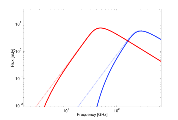
Figure 5.— Theoretical radio spectra of SNe including synchrotron-self absorption and with (solid lines) or without (dashed lines) free-free absorption. Blue and red lines are for days 1 and 4 after explosion, respectively. The above spectra were produced using Equations 5, A5 and A8 with the fitted parameters found in $\S 3.2$ for SN 2011dh.

If had we observed SN 2011dh on day 1 the EVLA observations would have shown clear signature for free-free absorption. We also note that $\tau_{\rm ff}$ is proportional to $n_{*}^{2}r_{*}$ whereas the SSA optical depth is a different function of $n_{*}$ and $r_{*}$. Thus we can, in principle, obtain a different measure of $n_{*}$ and $r_{*}$.

References

- Arcavi et al. (2011) Arcavi, I., et al. 2011a, The Astronomer’s Telegram, 3413, 1
- Arcavi et al. (2011) Arcavi I., et al., 2011b, ApJ, 742, L18
- Arnaud (1996) Arnaud, K. A. 1996, Astronomical Data Analysis Software and Systems V, 101, 17
- Burrows et al. (2003) Burrows, D. N., et al. 2003, Proc. SPIE, 4851, 1320
- Chevalier & Soderberg (2010) Chevalier, R. A., & Soderberg, A. M. 2010, ApJ, 711, L40
- Chevalier & Fransson (2006) Chevalier R. A., Fransson C., 2006, ApJ, 651, 381
- Chevalier (1998) Chevalier, R. A. 1998, ApJ, 499, 810
- Chevalier (1982) Chevalier, R. A. 1982, ApJ, 259, 302
- Chevalier (1981) Chevalier R. A., 1981, ApJ, 251, 259
- Evans et al. (2007) Evans, P. A., et al. 2007, A&A, 469, 379
- Katz (2012) Katz B., 2012, MNRAS, 420, L6
- Krauss et al. (2012) Krauss M. I., et al., 2012, ApJ, 750, L40
- Law et al. (2009) Law, N. M., et al. 2009, PASP, 121, 1395
- Maund et al. (2011) Maund J. R., et al., 2011, ApJ, 739, L37
- Oke et al. (1995) Oke J. B., et al., 1995, PASP, 107, 375
- Perley et al. (2011) Perley R. A., Chandler C. J., Butler B. J., Wrobel J. M., 2011, ApJ, 739, L1
- Pooley (2011) Pooley D., 2011, ATel, 3456, 1
- Readhead (1994) Readhead A. C. S., 1994, ApJ, 426, 51
- Soderberg et al. (2012) Soderberg A. M., et al., 2012, ApJ, 752, 78
- Soderberg et al. (2010) Soderberg, A. M., Brunthaler, A., Nakar, E., Chevalier, R. A., & Bietenholz, M. F. 2010, ApJ, 725, 922
- Soderberg et al. (2006) Soderberg A. M., Chevalier R. A., Kulkarni S. R., Frail D. A., 2006, ApJ, 651, 1005
- Szczygieł et al. (2011) Szczygieł D. M., Gerke J. R., Kochanek C. S., Stanek K. Z., 2011, arXiv, arXiv:1110.2783
- Rau et al. (2009) Rau, A., et al. 2009, PASP, 121, 1334
- Van Dyk et al. (2011) Van Dyk S. D., et al., 2011, ApJ, 741, L28
- Weiler et al. (2002) Weiler, K. W., Panagia, N., Montes, M. J., & Sramek, R. A. 2002, ARA&A, 40, 387
- Weiler et al. (2007) Weiler K. W., Williams C. L., Panagia N., Stockdale C. J., Kelley M. T., Sramek R. A., Van Dyk S. D., Marcaide J. M., 2007, ApJ, 671, 1959