Black Hole Growth to $z=2$ - I: Improved Virial Methods for Measuring $M_{\rm BH}$ & $L/L_{\rm Edd}$

Abstract

We analyze several large samples of Active Galactic Nuclei (AGN) in order to establish the best tools required to study the evolution of black hole mass ($M_{\rm BH}$) and normalized accretion rate ($L/L_{\rm Edd}$). The data include spectra from the SDSS, 2QZ and 2SLAQ public surveys at $z<2$, and a compilation of smaller samples with $0<z<5$. We critically evaluate the usage of the Mg ii $\lambda 2798$ and C iv $\lambda 1549$ lines, and adjacent continuum bands, as estimators of $M_{\rm BH}$ and $L/L_{\rm Edd}$, by focusing on sources where one of these lines is observed together with H$\beta$. We present a new, luminosity-dependent bolometric correction for the monochromatic luminosity at 3000Å, $L_{3000}$, which is lower by a factor of $\sim 1.75$ than those used in previous studies. We also re-calibrate the use of $L_{3000}$ as an indicator for the size of the broad emission line region (${R_{\rm BLR}}$) and find that $\hbox{${R_{\rm BLR}}$}\propto L_{3000}^{0.62}$, in agreement with previous results. We find that ${\rm FWHM}\left({\rm Mg}{\textsc{ii}}\right)\simeq{\rm FWHM}\left({\rm H}\beta\right)$ for all sources with ${\rm FWHM}\left({\rm Mg}{\textsc{ii}}\right)\raisebox{-2.15277pt}{$\;\stackrel{{\scriptstyle<}}{{\sim}}\;$}6000\,{\rm km\,s}^{-1}$. Beyond this FWHM, the Mg ii line width seems to saturate. The spectral region of the Mg ii line can thus be used to reproduce H$\beta$-based estimates of $M_{\rm BH}$ and $L/L_{\rm Edd}$, with negligible systematic differences and a scatter of $\sim$0.3 dex. The width of the C iv line, on the other hand, shows no correlation with either that of the H$\beta$ or the Mg ii lines and we could not identify the reason for this discrepancy. The scatter of $M_{\rm BH}$(C iv), relative to $M_{\rm BH}$(H$\beta$) is of almost 0.5 dex. Moreover, 46% of the sources have ${\rm FWHM}\left({\rm C}\,\textsc{iv}\right)\raisebox{-2.15277pt}{$\;\stackrel{{\scriptstyle<}}{{\sim}}\;$}{\rm FWHM}\left({\rm H}\beta\right)$, in contrast with the basic premise of the virial method, which predicts ${\rm FWHM}\left({\rm C}\,\textsc{iv}\right)/{\rm FWHM}\left({\rm H}\beta\right)\simeq\sqrt{3.7}$, based on reverberation mapping experiments. This fundamental discrepancy cannot be corrected based on the continuum slope or any C iv-related observable. Thus, the C iv line cannot be used to obtain precise estimates of $M_{\rm BH}$. We conclude by presenting the observed evolution of $M_{\rm BH}$ and $L/L_{\rm Edd}$ with cosmic epoch. The steep rise of $L/L_{\rm Edd}$ with redshift up to $z\simeq 1$ flattens towards the expected maximal value of $L/L_{\rm Edd}\simeq 1$, with lower-$M_{\rm BH}$ sources showing higher values of $L/L_{\rm Edd}$ at all redshifts. These trends will be further analyzed in a forthcoming paper.

1 Introduction

The growth of Super-Massive Black Holes (SMBHs), which reside in the centers of most large galaxies, progresses through episodes of radiatively-efficient accretion, during which such systems appear as Active Galactic Nuclei (AGN). Many details of this growth process are still unknown. In the local Universe most AGN are powered by lower-mass BHs, with $M_{\rm BH}\sim 10^{6}-10^{8}\,M_{\odot}$, growing at very slow rates (e.g., Marconi et al., 2004; Hasinger et al., 2005; Netzer & Trakhtenbrot, 2007, hereafter NT07). It is thus clear that the more massive BHs accreted at higher rates in the past. Indeed, several studies suggest that the typical normalized accretion rates ($L/L_{\rm Edd}$) increase with redshift (e.g., Fine et al., 2006, NT07). In contrast, the few luminous $z\sim 6$ QSOs for which $M_{\rm BH}$ was measured show extremely high masses, of about $\sim 10^{9}\,M_{\odot}$, and high accretion rates, near their Eddington limit. These systems could have grown to be the most massive BHs known ($M_{\rm BH}\sim 10^{10}\,M_{\odot}$) as early as $z\sim 4$ (Willott et al., 2010; Kurk et al., 2007; De Rosa et al., 2011; Trakhtenbrot et al., 2011, hereafter T11).

For un-obscured, type-I AGN, $M_{\rm BH}$ can be estimated by so-called “single-epoch” or “virial” estimators. These methods rely on the results of reverberation-mapping (RM) experiments, which provide empirical relations between the emissivity-weighted radius of the Broad Line Region (BLR) and the source luminosity $L$. These $\hbox{${R_{\rm BLR}}$}-L$ relations are parametrized as $\hbox{${R_{\rm BLR}}$}\propto\left(\lambda L_{\lambda}\right)^{\alpha}$. Assuming the motion of the BLR gas is virialized, the single-epoch $M_{\rm BH}$ estimators take the general form

$$M_{\rm BH}=f\,G^{-1}\,\left(\lambda L_{\lambda}\right)^{\alpha}V_{\rm BLR}^{2}\,\,\,,$$ (1)

where $V_{\rm BLR}$ is a probe of the BLR velocity field and $f$ is a factor that depends on the geometrical distribution of the BLR gas. A common estimator of this type is the “H$\beta$ method” (hereafter $M_{\rm BH}$[$L_{5100}$]). Here ${R_{\rm BLR}}$ is estimated from $\lambda L_{\lambda}$ at 5100Å (hereafter $L_{5100}$), FWHM(H$\beta$) is the velocity proxy, and $\alpha=0.6\pm 0.1$ Kaspi et al. (2000, 2005); Bentz et al. (2009). Another method is based on the Mg ii $\lambda 2798$ line and the adjacent continuum luminosity ($L_{3000}$). Although the few Mg ii-dedicated reverberation campaigns have not yet revealed a robust $\hbox{${R_{\rm BLR}}$}-L_{3000}$ relation (e.g., Clavel et al., 1991; Metzroth et al., 2006), several studies calibrated the Mg ii relation by using UV spectra of sources that have H$\beta$ reverberation data. One particular example is the relation presented in McLure & Jarvis (2002), and later refined by McLure & Dunlop (2004, hereafter MD04). The “H$\beta$” and “Mg ii” estimators were used in numerous papers to derive $M_{\rm BH}$ for many thousands of sources. This means focusing on either $z\lesssim 0.75$ or $0.75\lesssim z\lesssim 2$ AGN (e.g., Croom et al., 2004; Fine et al., 2006; Shen et al., 2008; Rafiee & Hall, 2011). Other studies used these estimators for small samples of sources at higher redshifts, where the lines are observed in one of the NIR bands Shemmer et al. (2004); Netzer et al. (2007); Kurk et al. (2007); Marziani et al. (2009); Dietrich et al. (2009); Willott et al. (2010).

In principal, $M_{\rm BH}$ can also be estimated from the broad C iv $\lambda 1549$ line, since ${R_{\rm BLR}}$(C iv) is known from RM experiments (e.g., Kaspi et al., 2007). A specific calibration of this type is given in Vestergaard & Peterson (2006) and several other papers. Such methods would potentially enable the study of large samples of AGN at $1.5\raisebox{-2.15277pt}{$\;\stackrel{{\scriptstyle<}}{{\sim}}\;$}z\raisebox{-2.15277pt}{$\;\stackrel{{\scriptstyle<}}{{\sim}}\;$}5$ for which C iv is observed in large optical surveys (e.g., Vestergaard et al., 2008; Vestergaard & Osmer, 2009). However, there is evidence that such C iv-based estimates are highly uncertain. In particular, Baskin & Laor (2005, hereafter BL05) found that the C iv line is often blue-shifted with respect to the AGN rest-frame, and that FWHM(C iv) is often smaller than FWHM(H$\beta$), both indicating that the dynamics of the C iv-emitting gas may be dominated by non-virial motion A later study by Vestergaard & Peterson (2006) claimed that at least some of these findings may be due to the inclusion of narrow-line objects and low-quality spectra in the BL05 sample. Despite this reservation, several subsequent studies of large, flux-limited samples clearly demonstrated that the relation between the widths of the C iv and Mg ii lines shows considerable scatter and, as a result, the C iv-based estimates of $M_{\rm BH}$ can differ from those deduced from Mg ii by up to an order of magnitude Shen et al. (2008); Fine et al. (2010). Moreover, studies of small samples of $z\sim 2-3.5$ AGN by, e.g., (Netzer et al., 2007, N07 hereafter), (Shemmer et al., 2004, S04 hereafter) and (Dietrich et al., 2009, D09 hereafter), show that the large discrepancies between C iv and H$\beta$ mass estimates persist even in high-quality spectra of broad-line AGN (i.e. where ${\rm FWHM}\left({\rm H}\beta\right)\raisebox{-2.15277pt}{$\;\stackrel{{\scriptstyle>}}{{\sim}}\;$}4000\,{\rm km\,s}^{-1}$). These issues were investigated in a recent study by Assef et al. (2011), which suggested an empirical correction for the C iv-based estimators that is based on the shape of the observed UV-optical spectral energy distribution (SED). This correction, however, may turn impractical for large optical surveys of high redshift AGN, where only the rest-frame UV regime is observed.

In this paper, we re-examine the methods used to derive $M_{\rm BH}$ and $L/L_{\rm Edd}$ of high-redshift type-I AGN. We discuss both large and small samples, including some that were never presented in this context. The various samples are described in §2 and the measurement procedures in §3. We discuss the monochromatic luminosities and bolometric corrections in §4. We briefly discuss the premise of the virial assumption in for estimating $M_{\rm BH}$ in §5. In §6 we examine how the Mg ii emission line complex can be used to measure $M_{\rm BH}$, and in §7 we provide new evidence regarding the fundamental limitations of the C iv method. Finally, in §8 we briefly describe the observed evolution of $M_{\rm BH}$ and $L/L_{\rm Edd}$, as measured with the tools developed in this paper, and summarize our conclusions. A more detailed analysis of the evolutionary trends is deferred to a forthcoming paper. Throughout this work we assume a cosmological model with $\Omega_{\Lambda}=0.7$, $\Omega_{\rm M}=0.3$, and $H_{0}=70\,{\rm km\,s}^{-1}\,{\rm Mpc}^{-1}$.

2 Samples Selection

The main goal of the present work is to test how the Mg ii $\lambda 2798$ and C iv $\lambda 1549$ emission line complexes can be used to estimate $M_{\rm BH}$, $L_{\rm bol}$ and $L/L_{\rm Edd}$, and to apply these methods to probe the evolution of $L/L_{\rm Edd}$ to $z\simeq 2$. While Mg ii can be compared to H$\beta$ or C iv within the same spectroscopic window (at $z\sim 0.6$ or $z\sim 1.7$, respectively), the comparison between C iv and H$\beta$ has to be based on a combination of separate observations. This dictates two distinct types of samples: (1) large samples drawn from the Sloan Digital Sky Survey (SDSS; York et al., 2000), 2dF QSO Redshift survey (2QZ; Croom et al., 2004) and the 2dF SDSS LRG And QSO survey (2SLAQ; Richards et al., 2005; Croom et al., 2008) catalogs; and (2) several smaller AGN samples, with publicly available data. The following details all the samples used in the paper, which are summarized in Table 1. We note that the 2QZ and 2SLAQ surveys provided relatively few high-quality spectra, which are usable for the comparisons between the different lines (see below). All the spectra analyzed in the present work were corrected for galactic extinction using the maps of Schlegel et al. (1998) and the model of Cardelli et al. (1989).

2.1 SDSS DR7

We queried the public catalogs of the seventh data release of the SDSS (DR7; Abazajian et al., 2009) for all sources that are classified as “QSO” and have a high confidence redshift determination (i.e. zconf$>0.7$) in the range of $z<2$. This resulted in 74517 sources. First, we omitted from this sample 7845 objects for which the line fitting procedures resulted in poor-quality fits, similarly to our criteria in NT07 (see more details in §3). Next, we omitted from our analysis all radio-loud sources. The radio loudness of each source, $R_{\rm L}\equiv f_{\nu}\left(5\,\rm{GHz}\right)/f_{\nu}\left(4400\rm{\AA}\right)$ (following Kellermann et al., 1989), was derived from the FIRST data Becker et al. (1995); White et al. (1997) incorporated in the SDSS public archive. For sources at $z>1$, we estimated $f_{\nu}\left(4400\rm{\AA}\right)$ using the continuum flux density near 2200Å and by assuming $f_{\nu}\propto\nu^{-0.44}$ (Vanden Berk et al., 2001, VdB01 hereafter). We removed all sources with $R_{\rm L}>10$ from our sample.

Finally, we omitted 1764 sources that are classified as broad absorption line QSOs (BALQSOs), based on their Mg ii and/or C iv spectral regions. For this, we used the relevant flags in the SDSS/DR7 catalog of Shen et al. (2011, see below) that, in turn, is largely based on the SDSS/DR5 catalog of BALQSOs of Gibson et al. (2009), with further (manual and hence partial) classification of the post-DR5 spectra. Although the Shen et al. (2011) BALQSO classification is probably incomplete, its combination with our fit quality criteria provide a sample which is almost completely BALQSO-free.

The final SDSS sample comprises 20894 for which H$\beta$ is observed ($z<0.75$) and 43995 sources for which only the Mg ii line is observed (i.e. $0.75<z<2$). There are 6731 sources for which both the H$\beta$ and Mg ii lines are observed ($0.5<z<0.75$; the SDSS “H$\beta$$\times$Mg ii” sub-sample hereafter) and 10910 sources where both the Mg ii and C iv lines are observed ($1.5<z<1.95$; the SDSS “Mg ii$\times$C iv” sub-sample hereafter).

The general SDSS sample significantly overlaps with the sample studied by Shen et al. (2011). Virtually all our $z>0.75$ sources are found within the Shen et al. (2011) catalog, in particular about 98% of our SDSS “H$\beta$$\times$Mg ii” and “Mg ii$\times$C iv” sub-samples, which have $M_{\rm BH}$ derived from more than one emission line in that catalog. At lower redshifts the fractions are lower, and only $\sim 68\%$ of our H$\beta$-only SDSS sources can be found within the Shen et al. (2011) catalog. This is due to our choice to include relatively faint sources that were excluded from the Shen et al. (2011) catalog, namely sources with $M_{i}\geq-22$ (see also Schneider et al., 2010). We verified that these faint sources have high-quality H$\beta$ fits, according to our criteria (see §3). In addition, we note that our SDSS “H$\beta$$\times$Mg ii” sub-sample includes 354 of the 495 sources ($\sim 75\%$) analyzed in the study by Wang et al. (2009). The discrepancy is due to the fact that Wang et al. (2009) chose to include in their sample sources with slightly lower redshifts ($0.45<z<0.75$). Our general (H$\beta$) SDSS sample includes 473 of their sources ($\sim 95\%$).

Table 1: Summary of Samples

			Lines useda			Sizes of cross-calibration samples
Name (Acc.)	${\rm N}_{\rm Total}$	$z$	H$\beta$	Mg ii	C iv	H$\beta$$\times$Mg ii	Mg ii$\times$C iv	H$\beta$$\times$C iv
SDSS	66653	$0-2$	$s$	$s$	$s$	6731	10910	$-$
2QZ	9111	$0.35-1.7$	$s$	$s$	$s$	238	489	$-$
2SLAQ	2287	$0.45-1.6$	$s$	$s$	$s$	39	217	$-$
Baskin & Laor (2005, BL05)	59	$0.25-0.5$	$s$	$-$	$t$	$-$	$-$	81
Netzer et al. (2007, N07)b	44	$2.2-3.5$	$s$	$-$	$s$	$-$	$-$	44
Shang et al. (2007, Sh07)	22	$0.1-0.4$	$t$	$t$	$t$	22	22	22
Sulentic et al. (2007, Sul07)	90	$<1$	$t/s$	$s$	$t$	9	11	57
McGill et al. (2008, Mc08)	19	$\sim 0.36$	$t$	$t$	$-$	19	$-$	$-$
Dietrich et al. (2009, D09)	10	$1-2.2$	$t$	$t$	$t$	7	7	9
Marziani et al. (2009, M09)	30	$1-2.4$	$t$	$s$	$s$	16	12	6
Trakhtenbrot et al. (2011, T11)	40	$\sim 4.8$	$-$	$s$	$s$	$-$	40	$-$
a Type of data used: “t” - tabulated data; “s” - spectra fitted by our team (i.e., this work, Shemmer et al., 2004, N07 and T11).
b The majority of sources in this sample were presented in Shemmer et al. (2004).

2.2 2QZ

We used the public 2QZ catalog of Croom et al. (2004), initially choosing all $0.5<z<2$ sources which are classified as “QSO” and have high confidence redshift determination (i.e. ZQUAL flag better than 22). Our query naturally omits BALQSOs, which are classified as such within the 2QZ catalog (based on visual inspection of the spectra, which is incomplete; see Croom et al., 2004). This query provided 20315 sources. After applying the fit quality criteria to this large Mg ii 2QZ sample, it comprises 8873 sources. Generally, spectra obtained as part of the 2QZ and 2SLAQ AAO-based surveys are not flux calibrated. Previous studies used single-band magnitudes, in either the ${\rm B}_{\rm J}$ or the $g$ bands, to derive monochromatic luminosities, assuming all spectra follow a uniform UV-to-optical SED of $f_{\rm\nu}\sim\nu^{-0.5}$ (e.g., Croom et al., 2004; Richards et al., 2005; Fine et al., 2008). Here we employed a more robust flux calibration scheme, which relies on all the photometric data available in the 2QZ and 2SLAQ catalogs. This procedure is discussed in Appendix A.

In order to expand the luminosity range of the “H$\beta$$\times$Mg ii” sample, we preformed a separate query of all $0.35<z<0.55$ 2QZ sources, ignoring their class and ZQUAL. For the selection of “Mg ii$\times$C iv” sources we focused on sources at $1.5<z<1.8$ (within the larger Mg ii sample) These choices were made in order to include sources which might be flagged as problematic due to the proximity of the H$\beta$ line to the telluric features near 7000Å or to the limit of the observed spectral range, and to avoid these problems from affecting the C iv line. The “H$\beta$$\times$Mg ii” sources which passed the fit quality criteria were manually inspected, to omit any non-QSO objects or otherwise unreliable spectra. These procedures resulted in merely 238 sources with reliable H$\beta$ fits and 489 sources with reliable C iv fits.

To summarize, we have 9111 2QZ sources in our final sample, 238 of which have both H$\beta$ and Mg ii, and 489 sources with both Mg ii and C iv. These sources span the magnitude range $b_{\rm J}\sim 18-20.85$, which corresponds to the luminosity range $44\lesssim\log\left(L_{\rm bol}/{\rm erg\,s}^{-1}\right)\lesssim 46$ at $z\simeq 1.5$ (see §4.2). The 2QZ sample thus reaches about a factor $3.75$ deeper than the SDSS sample.

2.3 2SLAQ

Sources from the 2SLAQ survey were selected by using the public 2SLAQ QSO catalog, compiled and presented in Croom et al. (2008), and further analyzed in Fine et al. (2010). Our query focused on $0.5<z<1.8$ sources which are classified as “QSO”, and resulted in 5873 sources. Here too, BALQSOs are largely omitted, due to their separate classification. Low-redshift 2SLAQ sources suffer from the same limitations affecting the 2QZ low-redshift sources. We preformed a separate search to locate “H$\beta$$\times$Mg ii” candidates at $0.4<z<0.6$. Our careful manual inspection resulted in only 39 sources with reasonable fits to both the H$\beta$ and Mg ii lines. We chose not to include any of these sources in the present analysis, due to their poor S/N and small number. Sources with $1.5<z<1.65$ in the large Mg ii sample have both Mg ii and C iv. We have 217 such sources, out of a total of 2287. These sources span the magnitude range $g\sim 18-22$, which corresponds to $44\lesssim\log\left(L_{\rm bol}/{\rm erg\,s}^{-1}\right)\lesssim 46$ at $z\simeq 1.5$. This is almost an order of magnitude deeper than SDSS, and about a factor of 2.5 deeper than 2QZ.

2.4 Additional Samples

There are many smaller samples in the literature with measurements of more than one of the three emission lines discussed here. We choose to focus on samples for which the relevant line measurements are either preformed by procedures very similar to ours and publicly tabulated, or on samples for which such measurements could be preformed on publicly available spectra. In particular, we used the samples of BL05 (59 sources), N07 (and S04; 44 sources), Shang et al. (2007, hereafter Sh07 hereafter; 22 sources), Sulentic et al. (2007, hereafter Sul07; 90 sources), McGill et al. (2008, hereafter Mc08; 19 sources), Dietrich et al. (2009, hereafter D09; 10 sources), Marziani et al. (2009, hereafter M09; 30 sources), and T11 (40 sources). Basic information on these samples is given in Table 1, while Appendix B provides more details regarding the acquisition and contents of the samples. In particular, Appendix B details which line measurements we used cases where sources appeared in more than one sample.

These small samples probe a wide range of redshift and luminosity and most of them have higher S/N than those typically obtained within the large SDSS, 2QZ and 2SLAQ surveys. In many of these samples the different lines were not observed simultaneously. Thus, it is possible that line and/or continuum variability contributes to the scatter in the relationships discussed in this work.

3 Line and Continuum Fitting

We have developed a set of line fitting procedures to derive the physical parameters related to the H$\beta$, Mg ii and C iv lines. These procedures are similar in many ways to those described in previous publications (e.g., S04, N07, NT07, S08, F08). In particular, the H$\beta$ and Mg ii fitting procedures follow those used in NT07 and T11, respectively. In short, a linear continuum model is fitted to the flux densities in two 20Å-wide “bands” on both side of the relevant emission line. The bands are centered around 4435 & 5110Å for H$\beta$, 2655 & 3020Å for Mg ii and 1450 & 1690Å for C iv. For the H$\beta$ and Mg ii lines, we subtract a template of Fe ii and Fe iii emission lines. This is done by choosing the best-fit broadened and shifted template based on data published by Boroson & Green (1992) and Vestergaard (2004). The grid spans a broad range both in the width and (velocity) shift of the iron features. In the case of Mg ii, we add flux in the wavelength range under the emission line itself (see Appendix C.2) The main emission lines are modeled by a combination of two broad and one narrow Gaussians. In the cases of Mg ii and C iv this model is duplicated for each of the doublet components. In Appendix C we discuss several minor but important technical issues concerning the fitting of the lines, including: (1) the ranges of all relevant parameters; (2) the narrow ($\raisebox{-2.15277pt}{$\;\stackrel{{\scriptstyle<}}{{\sim}}\;$}1000\,{\rm km\,s}^{-1}$) components of all lines; (3) the improved iron template for the Mg ii spectral complex and its scaling; (4) the difference between our fitted $L_{3000}$ and the “real” power-law continuum, and (5) the emission features surrounding the C iv line.

All fitting procedures were tested on several hundred spectra, selected from all samples used here. For these, we individually inspected the fitted spectra. In particular, we verified that the simplifications involved in the C iv fitting procedure (Appendix C.3) are justified. After fitting the SDSS, 2QZ and 2SLAQ samples, we filtered out low-quality fits by imposing the criteria $\chi^{2}<5$ and $R^{2}>0.2$. Both these quantities were calculated over a range of $14000\,{\rm km\,s}^{-1}$ centered on the peaks of the relevant emission lines, and adjusted for degrees of freedom. This choice is similar to the one we made in our previous analysis of large samples (NT07). The smaller samples were treated manually, securing high-quality fitting results for all sources where adequate spectral coverage of the various lines was available. We stress that even when two of the three main lines are observed in the same spectrum (i.e. for the “H$\beta$$\times$Mg ii” and “Mg ii$\times$C iv” sub-samples), the fitting procedures are ran separately for each emission line complex. Thus, the parameters of the different models are fully independent, even when it is possible to assume otherwise.

The line fitting procedures provide monochromatic luminosities ($L_{1450}$, $L_{3000}$ and/or $L_{5100}$) and emission lines widths. For the latter, we calculated the FWHM, the line dispersion $\sigma$ (following Peterson et al., 2004) and the inter-percentile velocity (IPV; following Croom et al., 2004). We estimated ${R_{\rm BLR}}$ for all the sources for which the “H$\beta$ method” is applicable, by:

$$\hbox{${R_{\rm BLR}}$}\left({\rm H}\beta\right)=538.2\left(\frac{L_{5100}}{10^{46}\,{\rm erg\,s}^{-1}}\right)^{0.65}\,\,{\rm lt-days}\,.$$ (2)

This is an updated version of the correlation found by Kaspi et al. (2005), taking into account the improved measurements presented in Bentz et al. (2009), but fitting the RM measurements of only the sources with $L_{5100}\raisebox{-2.15277pt}{$\;\stackrel{{\scriptstyle>}}{{\sim}}\;$}10^{44}\,{\rm erg\,s}^{-1}$, typical of the luminosities of high-redshift sources. $M_{\rm BH}$(H$\beta$) is derived by assuming $f=1$ (Netzer & Marziani, 2010, and references therein) and is given by:

$$M_{\rm BH}\left({\rm H}\beta\right)=1.05\times 10^{8}\left(\frac{L_{5100}}{10^{46}\,{\rm erg\,s}^{-1}}\right)^{0.65}\left[\frac{{\rm FWHM}\left({\rm H}\beta\right)}{10^{3}\,{\rm km\,s}^{-1}}\right]^{2}\,\,M_{\odot}\,\,.$$ (3)

We have also experimented with flatter ${R_{\rm BLR}}$-$L_{5100}$ relations, of $\hbox{${R_{\rm BLR}}$}\propto L_{5100}^{0.5}$, as suggested by some studies (e.g. Bentz et al., 2009). We found, as in Kaspi et al. (2005), that these have little effect on our main results, provided that the constant in Eq. 2 is adjusted accordingly. In particular, for the median luminosity of the SDSS “H$\beta$$\times$Mg ii” sub-sample ($L_{5100}=6\times 10^{44}\,{\rm erg\,s}^{-1}$) the ${R_{\rm BLR}}$-$L_{5100}$ relation of Bentz et al. (2009) would have resulted in ${R_{\rm BLR}}$ estimates that are larger by 0.03 dex than the ones obtained by Eq. 2. For the “H$\beta$$\times$C iv” and “Mg ii$\times$C iv” sub-samples we assumed the reverberation-based relation of Kaspi et al. (2007):

$$\hbox{${R_{\rm BLR}}$}\left({\rm C}\,\textsc{iv}\right)=107.2\left(\frac{L_{1450}}{10^{46}\,{\rm erg\,s}^{-1}}\right)^{0.55}\,\,{\rm lt-days}\,\,.$$ (4)

We also experimented with the relation of Vestergaard & Peterson (2006), $\hbox{${R_{\rm BLR}}$}\propto L_{1450}^{0.53}$, and verified that none of the results that follow depend on this choice.

4 Luminosities and Bolometric Corrections

4.1 Monochromatic Luminosities and SED Shapes

The UV-optical continuum emission of type-I AGN, between $\sim$1300 and 5000Å is well described by $f_{\nu}\propto\nu^{-0.5}$ (e.g., VdB01). The typical luminosity scaling values in our SDSS sample are $\left<L_{3000}/L_{5100}\right>=1.62$ and $\left<L_{1450}/L_{3000}\right>=1.39$, with standard deviations of 0.12 and 0.14 dex, respectively. Assuming the average conversion of $L_{3000}$ to the “real” continuum (see Appendix C.2), these ratios become $\left<L_{3000}/L_{5100}\right>=1.41$ and $\left<L_{1450}/L_{3000}\right>=1.59$, respectively. For comparison, the ratios implied by an $\alpha_{\nu}=-0.5$ power law are 1.30 and 1.44, respectively. Figure 1 shows that the smaller “H$\beta$$\times$C iv” sub-samples generally follow the scalings of $\alpha_{\nu}\simeq-0.5$. However, the ratio of $L_{1450}/L_{5100}\simeq 1.95$ provides a somewhat better scaling for these sources, for which both $L_{5100}$ and $L_{1450}$ are directly observed. This ratio is consistent with the VdB01 result, which is based on a composite of sources for which either $L_{5100}$ or $L_{1450}$ were observed. In particular, all the PG quasars that are part of the reverberation-mapped sample of Kaspi et al. (2000) follow these luminosity scalings (these are part of the BL05, Sh07 and Sul07 samples). Thus, we do not expect that SED differences would play a major role in scaling any relation that is consistent with the RM experiments. This is a crucial point in single-epoch $M_{\rm BH}$ determinations and is further discussed in §7.

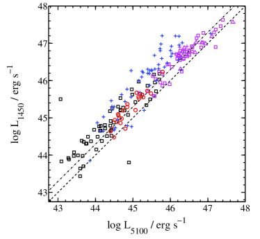
Figure 1: A comparison between $L_{1450}$ and $L_{5100}$ for for the different “H$\beta$$\times$C iv” samples: BL05 (black squares), N07+S04 (magenta squares), Sh07 (red circles), Sul07 (blue crosses) D09 (magenta crosses) and M09 (magenta triangles; see Table 1 for references and details). The dashed line represents the 1:1 relation, and the dot-dashed line represents $L_{1450}=1.97\,L_{5100}$, the median value found for the N07+S04 sample, and typical for other high-luminosity sources. A power-law continuum with $\alpha_{\nu}=-0.5$ (e.g. Vanden Berk et al., 2001) would imply $L_{1450}=1.88\,L_{5100}$.

We note that 87% of the sources in the SDSS “Mg ii$\times$C iv” sub-sample have $L_{1450}>L_{3000}$, and 93% of the sources in the smaller “Mg ii$\times$C iv” sub-samples (Sh07, BL05, N07+S04, M09 & D09) have $L_{1450}>L_{5100}$ (i.e., $\alpha_{\nu,{\rm UVO}}>-1$). In contrast, half of the sources (6/12) presented by Assef et al. (2011) have $L_{1450}\lesssim L_{5100}$. Such extreme UV-optical SEDs may represent AGN with intrinsically different properties or, perhaps, are affected by a higher-than-typical reddening. These issues are further discussed in §7.

4.2 Bolometric Corrections

To determine the bolometric luminosity ($L_{\rm bol}$) one has to assign a bolometric correction factor, $f_{\rm bol}\left(\lambda\right)=L_{\rm bol}/\lambda L_{\lambda}$. Here we focus on $f_{\rm bol}\left(3000{\rm\AA}\right)$. Several earlier studies assumed a constant $f_{\rm bol}\left(3000{\rm\AA}\right)$, e.g., $\sim 5.9$ Elvis et al. (1994), or $\sim 5.15$ Richards et al. (2006a). There are two problems with this approach: (1) The constant $f_{\rm bol}\left(3000{\rm\AA}\right)$ was based on the total, observed X-ray to mid-IR (MIR) SED of AGN. As such, it includes double-counting of part of the AGN radiation (the MIR flux originates from re-processing of the UV-optical radiation). This results in overestimation of $L_{\rm bol}$ and thus $f_{\rm bol}$ (e.g., Marconi et al., 2004). (2) The shape of the SED is known to be luminosity-dependent. This dependence is most significant at the X-ray regime, and perhaps also at UV wavelengths (e.g., Vignali et al., 2003). The general trend is of a decreasing $L_{\rm X}$ with increasing $L_{\rm UV-opt}$. Thus, $f_{\rm bol}$ should decrease with increasing UV luminosity. Marconi et al. (2004) provides a luminosity-dependent prescription for estimating $f_{\rm bol}$(4400Å) that addresses these two issues. The prescription can be modified to other wavelengths, by assuming a certain UV-optical SED.

We derived a new prescription for $f_{\rm bol}\left(3000{\rm\AA}\right)$ by using the SDSS “H$\beta$$\times$Mg ii” sub-sample. First, we converted the measured $L_{5100}$ of each source to $L_{\rm bol}$ using the prescription of Marconi et al. (2004) and assuming $f_{\nu}\propto\nu^{-0.5}$. This provides, for each of the 6731 sources, $L_{3000}$ and $L_{\rm bol}$/$L_{3000}$, which are presented in Figure 2. The derived bolometric corrections are systematically lower than the aforementioned fixed values. For example, the typical correction is just 3.4 for sources with $\log\left(L_{3000}/{\rm erg\,s}^{-1}\right)\simeq 3\times 10^{45}\,{\rm erg\,s}^{-1}$, which is the median luminosity of the SDSS sources at $z\simeq 1.2$. This is a factor of 1.5 lower than the value of 5.15 used in several other studies of $L/L_{\rm Edd}$ at $z\sim 1-2$ (e.g., Fine et al., 2008). Fig. 2 further reveals that, despite the large scatter at low $L_{3000}$, there is a clear trend of decreasing $f_{\rm bol}\left(3000{\rm\AA}\right)$ with increasing $L_{3000}$, as expected. To quantify this trend, we grouped the data in bins of 0.2 dex in $L_{3000}$ and assumed that the error on $f_{\rm bol}\left(3000{\rm\AA}\right)$ is $\sigma_{\rm i}/\sqrt{N_{\rm i}}$, for the i-th bin in $L_{3000}$. An ordinary least squares (OLS) fit to the binned data points gives:

f_bol(3000Å)$$=4.12-2.13{\cal L}_{3000,45}$$ (5)

$$+1.76{\cal L}_{3000,45}^{2}-0.54{\cal L}_{3000,45}^{3}\,,$$

where ${\cal L}_{3000,45}\equiv\log\left(L_{3000}/10^{45}\,{\rm erg\,s}^{-1}\right)$. As Fig. 2 clearly shows, this relation predicts relatively large bolometric corrections for low-luminosity sources, to the extreme of $f_{\rm bol}\left(3000{\rm\AA}\right)\raisebox{-2.15277pt}{$\;\stackrel{{\scriptstyle>}}{{\sim}}\;$}9.5$ for $L_{3000}\lesssim 10^{44}\,{\rm erg\,s}^{-1}$. Similarly high values were reported in the past, for a small minority of sources (e.g., Richards et al., 2006a). We suspect that the high values predicted by Eq. 5 are the result of unrealistic extrapolation of the Marconi et al. (2004) $L_{\rm B}-L_{\rm bol}$ relation towards low luminosities, where the number of measured points is small. Moreover, we note that low-luminosity sources may suffer from more significant host-galaxy contamination, which results in a systematic over-estimation of $L_{5100}$ and $L_{\rm bol}$. We thus caution that the bolometric corrections we provide here should not be used for sources with $L_{3000}\lesssim 10^{44}\,{\rm erg\,s}^{-1}$, where the emission from the host galaxy is comparable to that of the AGN and in particular in cases where the spectroscopic aperture affects the determination of the host emission (see, e.g., the analysis in Stern & Laor, 2012).

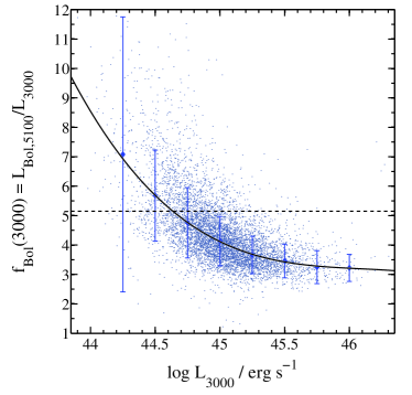
Figure 2: The relation between the empirically derived bolometric corrections ($f_{\rm bol}\left(3000{\rm\AA}\right)\equiv L_{\rm bol}/L_{3000}$) and $L_{3000}$, for the SDSS “H$\beta$$\times$Mg ii” sub-sample. Large symbols and error bars represent the binned data and the corresponding scatter (standard deviations). The solid black line represents the best-fit cubic polynomial to the binned data, given in Eq. 5. The dashed horizontal line represents $f_{\rm bol}\left(3000{\rm\AA}\right)=5.15$, the value used in several earlier studies (e.g., Richards et al., 2006a).

Figure 3 compares the bolometric luminosities derived from $L_{3000}$ by using Eq. 5 to those calculated from $L_{5100}$. The two methods provide consistent estimates of $L_{\rm bol}$ with a scatter of less than 0.09 dex (standard deviation of residuals). The small scatter is probably dominated by the range of UV-to-optical slopes of individual sources.

We finally note that the real uncertainties on such estimates of $L_{\rm bol}$ are actually governed by the range of global SED variations between sources, as well as the assumed physical (or empirical) model for the UV SED. For example, the assumed exponent of the X-ray model and the $L_{\rm X}-L_{\rm UV}$ relation may amount up to $\sim$0.2 dex in $L_{\rm X}$, and thus in the calculated $L_{\rm bol}$ (see, e.g., Vignali et al., 2003; Bianchi et al., 2009). Two very recent studies further demonstrated these complications. The study by Runnoe et al. (2012) showed that even the uniform Elvis et al. (1994) and Richards et al. (2006a) SEDs may provide $f_{\rm bol}\left(3000{\rm\AA}\right)$ as low as $\sim 3$, given that the integration is limited to $\lambda<1\,\mu{\rm m}$ (thus neglecting re-processed emission. However, the best-fit trends of Runnoe et al. (2012) predict $f_{\rm bol}\left(3000{\rm\AA}\right)\simeq 5.3$ for sources with $L_{3000}\simeq 10^{45}$, consistent with the commonly used value of 5.15. Jin et al. (2012) used an accretion disk fitting method that results in a much higher (unobserved) far-UV luminosity for a given optical and/or near-UV luminosity. Naturally, this model produced very high bolometric corrections, with $f_{\rm bol}\left(5100{\rm\AA}\right)\raisebox{-2.15277pt}{$\;\stackrel{{\scriptstyle>}}{{\sim}}\;$}12$ (and as high as $\sim$20-30) for several sources with $L_{5100}\simeq 3\times 10^{44}\,{\rm erg\,s}^{-1}$, compared to the Marconi et al. (2004) prediction of $f_{\rm bol}\left(5100{\rm\AA}\right)\simeq 7$. This completely new approach to the estimate of $L_{\rm bol}$ in AGN will not be further discussed in the present paper. Instead, we advice the usage of the corrections given by Eq. 5, which supplement the optical corrections of Marconi et al. (2004).

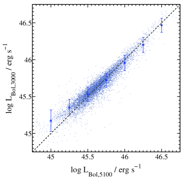
Figure 3: A comparison of estimates of $L_{\rm bol}$ based on $L_{3000}$ and $L_{5100}$, for the SDSS “H$\beta$$\times$Mg ii” sample. Large symbols and error bars represent the binned data and the corresponding scatter (standard deviations). The dashed line represents the the 1:1 relation.

5 Virial $M_{\rm BH}$ Estimates: Basic Considerations

A main goal of this paper is to present a critical evaluation of the various ways to measure $M_{\rm BH}$ by using the RM-based “virial” method. It is therefore important to review the basic premise of the method and the justifications for its use.

Four critical points should be considered:

1. The emissivity weighted radius of the BLR, ${R_{\rm BLR}}$, is known from direct RM-measurements almost exclusively for only the H$\beta$ and C iv emission lines, and to a much lesser extent for Mg ii (see §1). The expressions chosen for the present work are given in Eqs. 2 and 4. They depend on the measured $L_{5100}$ and $L_{1450}$, and involve the assumption that the derived luminosities require no reddening-related, or other, corrections. The slope $\alpha$ of these correlations ($\hbox{${R_{\rm BLR}}$}\propto L^{\alpha}$) is empirically determined to be in the range 0.5–0.7, by a simple regression analysis of the observational results. It is not known whether the fundamental dependence is on $L_{5100}$, $L_{1450}$, the ionizing luminosity or perhaps $L_{\rm bol}$, although there are theoretical justifications for all these cases. It is also not clear whether the slope itself depends on luminosity (i.e. whether the same relation holds for all luminosities, see, e.g., Bentz et al., 2009; Netzer & Marziani, 2010). Thus, the approach adopted here is to use all quantities as measured.

2. The mean ratio of the RM-based H$\beta$ and C iv radii, assuming the $\hbox{${R_{\rm BLR}}$}-L$ relations, is about 3.7. The number depends on the measured lags and the mean luminosities of the objects in the RM samples used to derive the relations, and may significantly vary for individual sources (see, e.g., the range of ratios in Peterson et al. 2004). The mean ratio of the two involved luminosities in the two RM samples is $L_{1450}/L_{5100}\sim 1.9$. This is similar to the mean ratio in several much larger samples where the two wavelength regions are observed (e.g., S04, BL05, N07; see §4.1) and is also similar to the SDSS-based composite spectrum of VdB01. The working assumption, therefore, is that this ratio represents the population of un-reddened type-I AGN well. Given this, the virial method cannot be applied directly to sources where $L_{1450}/L_{5100}$ deviates significantly from this typical value, since in such sources ${R_{\rm BLR}}$ may not scale with the luminosity in the same way as in the two RM samples used to derive the equations. For example, $L_{1450}/L_{5100}<<1.9$ may indicate significant continuum reddening, which will result in a systematic underestimation of ${R_{\rm BLR}}$, if one uses Eq. 4 or similar relations. Correcting for such reddening must be performed prior to the estimation of ${R_{\rm BLR}}$ or $M_{\rm BH}$.

3. The virial motion of the BLR, combined with the adoption of line FWHMs as the gas velocity indicator, and the assumption that the global geometry of the H$\beta$ and C iv parts of the BLR are similar (e.g. two spheres of different radii) lead to the prediction that ${\rm FWHM}\left({\rm C}\,\textsc{iv}\right)/{\rm FWHM}\left({\rm H}\beta\right)\simeq\sqrt{3.7}$. This is confirmed in a small number of intermediate luminosity objects showing the expected $L_{1450}/L_{5100}$ (e.g., Peterson et al., 2004). Given this, the simplest way to proceed to measure $M_{\rm BH}$ in large samples, which lack any additional information regarding the $L_{1450}/L_{5100}$ or ${\rm FWHM}\left({\rm C}\,\textsc{iv}\right)/{\rm FWHM}\left({\rm H}\beta\right)$ ratios, is to assume the same is true for all sources.

4. The best value of the geometrical factor $f$ in the mass equation (Eq. 1) is 1.0. This is an average value obtained from the comparison of RM-based “virial products” and the $M_{\rm BH}-\sigma_{*}$ relation, for about 30 low redshift type-I AGN (e.g., Onken et al., 2004; Woo et al., 2010; Graham et al., 2011). None of these sources show a large deviation from this value. These calibrations rely predominantly on H$\beta$, while C iv-related observables contribute to the estimation of virial products in only 5 sources. Unfortunately, there are no direct estimates of $f$ that are based solely on C iv.

   Given points (ii) and (iii) above, the value of $f$ used in $M_{\rm BH}$ estimates must be the same for the two emission lines. This is not meant to imply that certain sources cannot have two different virialized regions, for H$\beta$ and C iv, with different geometries and values of $f$. It only means that the method is based on certain samples with certain properties and hence should not be applied to objects with different properties. In objects where $f$ is not directly measured and the line width ratio deviate significantly from the above, e.g. objects with ${\rm FWHM}\left({\rm H}\beta\right)>{\rm FWHM}\left({\rm C}\,\textsc{iv}\right)$, at least one of the lines should not be used as a $M_{\rm BH}$ indicator within the framework of the virial method. Since estimates of $f$ based on FWHM(H$\beta$) are known to be correct in most of the H$\beta$-RM sample, we prefer to adopt in such cases the assumption that FWHM(H$\beta$) provides the more reliable mass indicator.

The above considerations suggest that a single epoch mass determination based on H$\beta$ and $L_{5100}$ is a reliable mass estimate provided there is no significant continuum reddening. In case the amount of reddening is known, it should be taken into account prior to the application of the method. In the absence of direct mass calibration based on lines other than H$\beta$, there are only two alternatives: use theoretical conjectures, or a-priori knowledge about the line width. The first can be used for the Mg ii line that is thought to originate from the same part of the BLR as H$\beta$. If ${\rm FWHM}\left({\rm Mg}{\textsc{ii}}\right)\simeq{\rm FWHM}\left({\rm H}\beta\right)$, then the line can be used for estimating $M_{\rm BH}$. The second can be used for the C iv line since $\hbox{${R_{\rm BLR}}$}({\rm C}\,\textsc{iv})/\hbox{${R_{\rm BLR}}$}({\rm H}\beta)$ is known. As explained, the requirement is ${\rm FWHM}\left({\rm H}\beta\right)/{\rm FWHM}\left({\rm C}\,\textsc{iv}\right)\simeq\sqrt{\hbox{${R_{\rm BLR}}$}\left({\rm C}\,\textsc{iv}\right)/\hbox{${R_{\rm BLR}}$}\left({\rm H}\beta\right)}$. If this ratio is indeed found in the majority of objects with measured FWHM(H$\beta$) and FWHM(C iv), then a single epoch mass estimate based on C iv can be safely used. In the following sections we use such considerations to assess the validity of the use of the Mg ii and C iv lines as mass indicators in type-I AGN.

6 Estimating $M_{\rm BH}$ with Mg ii $\lambda 2798$

As discussed in §5, the fact that there is no RM-based determination of ${R_{\rm BLR}}$(Mg ii) means that the only way to obtain a Mg ii-based estimator for $M_{\rm BH}$ is to calibrate it against $M_{\rm BH}$(H$\beta$), based on the the assumption that $\hbox{${R_{\rm BLR}}$}({\rm Mg}{\textsc{ii}})=\hbox{${R_{\rm BLR}}$}({\rm H}\beta)$ (verified by photoionization calculations). We therefore have to show that $L_{3000}$ can be used to estimate ${R_{\rm BLR}}$(H$\beta$), and that ${\rm FWHM}\left({\rm Mg}{\textsc{ii}}\right)\simeq{\rm FWHM}\left({\rm H}\beta\right)$. In what follows, we discuss these relations separately, and evaluate the ability of the (combined) virial product to reproduce $M_{\rm BH}$(H$\beta$).

6.1 Using $L_{3000}$ to Estimate ${R_{\rm BLR}}$

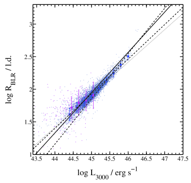
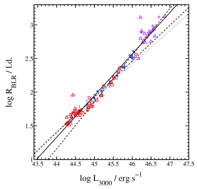
Figure 4: The relations between ${R_{\rm BLR}}$, estimated from $L_{5100}$, and $L_{3000}$, for the different “H$\beta$$\times$Mg ii” sub-samples under study. Left - large samples: blue and magenta points represent the SDSS and 2QZ “H$\beta$$\times$Mg ii” sub-samples, respectively. Larger symbols and error bars represent the binned data and the corresponding scatter (standard deviations). Right - small samples: the Sh07 (red circles), Mc08 (red triangles), D09 (magenta crosses) and M09 (magenta triangles) samples. The binned SDSS dataset is also included (blue diamonds and error bars). In both panels, the solid lines represent our best-fit relations (Eq. 7). Other lines provide reference for alternative relations: dashed lines represent our best-fit relations for either high- or low-luminosity sources (slopes of 0.695 and 0.531, respectively), while the dotted line represents a relation with a slope of 0.5 (normalized to match the median ${R_{\rm BLR}}$ of the SDSS “H$\beta$$\times$Mg ii” sub-sample at $L_{3000}=10^{45}\,{\rm erg\,s}^{-1}$). See the text and Table 2 for more details.

In Figure 4 we present the relation between the calculated values of ${R_{\rm BLR}}$(H$\beta$) and $L_{3000}$, for all the sources in the different “H$\beta$$\times$Mg ii” sub-samples. There is a clear and highly significant correlation between these two quantities. Since ${R_{\rm BLR}}$ is calculated directly from $L_{5100}$, this relation reflects the narrow distribution of UV-optical continuum slopes. To quantify the $\hbox{${R_{\rm BLR}}$}-L_{3000}$ relation, we bin the SDSS and 2QZ “H$\beta$$\times$Mg ii” sub-samples (separately) in bins of 0.2 dex in $L_{3000}$. The uncertainties on each binned data-point are assumed to be the standard deviations of the values included in the respective bin. The typical uncertainty is of 0.13 dex . This is a conservative choice, which attempts to account for the entire scatter in the data. All other “H$\beta$$\times$Mg ii” sub-samples remain un-binned. For these, we assume uncertainties of 0.1 dex on ${R_{\rm BLR}}$ and 0.05 dex on $L_{3000}$. These choices reflect the absolute flux calibration uncertainties and the uncertainties related to the continuum and line fitting processes. Since the uncertainties in both axes are comparable, we use the BCES Akritas & Bershady (1996) and FITEXY Press (2002) fitting methods, both designed to also take into account the scatter in the data. All the BCES correlations are tested by a bootstrapping procedure with 1000 realizations of the data under study. We used the more sophisticated version of the FITEXY method, as presented by Tremaine et al. (2002), where the error uncertainties on the data are scaled in order to account for the scatter. Thus, all our FITEXY correlations resulted in $\chi^{2}_{\nu}\simeq 1$. The best-fit linear relations (also shown in Fig. 4), parametrized as

$$\log\hbox{${R_{\rm BLR}}$}=\alpha\,\log\left(\frac{L_{3000}}{10^{44}\,{\rm erg\,s}^{-1}}\right)\,+\beta\,\,,$$ (6)

resulted in $\alpha\simeq 0.615$ and $\beta\simeq 1.33$ for both the BCES and FITEXY methods, The exact values and associated uncertainties are given in Table 2. The standard deviation of the residuals is about 0.1 dex. We note that some of the few low luminosity sources in Fig. 4 ($z<0.5$ sources from the Sh07 & Mc08 samples) appear to lie above our best-fit relation. This might be due to the contamination of their optical spectra by host light, which would cause their $L_{5100}$ (and hence ${R_{\rm BLR}}$) to be slightly overestimated, although effect should be very small ($<0.05$ dex; see, e.g., Sh07 and Bentz et al. (2009)). In addition, the few extremely high luminosity sources ($z>1.5$ sources from the D09 & M09 samples) also lie slightly above the best-fit relation of the combined dataset. Thus, the slope of the $\hbox{${R_{\rm BLR}}$}-L_{3000}$ relation may be somewhat shallower or steeper, in the low- or high-luminosity regimes, respectively. We tested these scenarios by re-fitting the data after omitting data points either above $L_{3000}=10^{46}\,{\rm erg\,s}^{-1}$ or below $L_{3000}=10^{45}\,{\rm erg\,s}^{-1}$, that is keeping most of the (binned) SDSS data but omitting the extreme sources from the “small” samples, on either side of the luminosity range. The results of this analysis are also presented in Table 2. In particular, we find that for sources with $L_{3000}\geq 10^{45}\,{\rm erg\,s}^{-1}$ the best-fit slope is $\alpha\simeq 0.7$, while for sources with $L_{3000}\leq 10^{46}\,{\rm erg\,s}^{-1}$ it is $\alpha\simeq 0.5$. Table 2 also lists best-fit parameters for other choices of sub-samples. In most of these cases, the derived slopes for the $\hbox{${R_{\rm BLR}}$}-L_{3000}$ relations are between those reported by McLure & Jarvis (2002) ($\alpha=0.47$) and by MD04 ($\alpha=0.62$). The intercepts are also very similar to those of McLure & Jarvis (2002), and the intercept derived from the entire dataset (1.33) differs from the one derived in MD04 by only 0.06 dex, in the sense that our best-fit relation predicts higher ${R_{\rm BLR}}$ values for a given value of $L_{3000}$. The MD04 study relation was derived using only sources with $L_{3000}>10^{44}\,{\rm erg\,s}^{-1}$, as is the case for most of the sources used here. Therefore, the differences between the MD04 relation and our results are not due to different luminosity regimes.

Table 2: Coefficients for ${R_{\rm BLR}}$-$L$ Correlations

	BCES bisector				FITEXY
Luminosity & sub-samples used	$\alpha$	$\beta$	$\sigma$ a	$M_{0}$ b	$\alpha$	$\beta$	$\sigma$ a
$x=\log\left(L_{3000}/10^{44}\,{\rm erg\,s}^{-1}\right)$
SDSS	$0.482\pm 0.004$	$1.440\pm 0.004$	$0.066$	$7.81$	$0.531\pm 0.004$	$1.388\pm 0.004$	$0.064$
SDSS+2QZ	$0.473\pm 0.005$	$1.450\pm 0.005$	$0.077$	$7.98$	$0.508\pm 0.003$	$1.415\pm 0.004$	$0.076$
“Small” b	$0.619\pm 0.014$	$1.340\pm 0.022$	$0.098$	$5.61$	$0.620\pm 0.015$	$1.334\pm 0.025$	$0.098$
SDSS (binned) + “Small” c	$0.618\pm 0.014$	$1.330\pm 0.020$	$0.094$	$5.62$	$0.619\pm 0.014$	$1.333\pm 0.023$	$0.094$
………$L_{3000}\leq 10^{46}\,{\rm erg\,s}^{-1}$	$0.531\pm 0.015$	$1.400\pm 0.019$	$0.071$	$6.93$	$0.544\pm 0.025$	$1.389\pm 0.029$	$0.071$
………$L_{3000}\geq 10^{45}\,{\rm erg\,s}^{-1}$	$0.695\pm 0.022$	$1.170\pm 0.037$	$0.087$	$4.67$	$0.701\pm 0.029$	$1.158\pm 0.059$	$0.087$
SDSS+2QZ (binned) + “Small” c	$0.615\pm 0.014$	$1.340\pm 0.019$	$0.093$	$5.66$	$0.618\pm 0.014$	$1.330\pm 0.023$	$0.093$
$x=\log\left(L\left({\rm Mg}{\textsc{ii}}\right)/10^{42}\,{\rm erg\,s}^{-1}\right)$
SDSS	$0.499\pm 0.006$	$1.38\pm 0.007$	$0.124$		$0.450\pm 0.005$	$1.428\pm 0.005$	$0.123$
SDSS+2QZ	$0.508\pm 0.007$	$1.36\pm 0.008$	$0.125$		$0.440\pm 0.005$	$1.436\pm 0.005$	$0.123$
“Small” d	$0.713\pm 0.034$	$1.13\pm 0.056$	$0.151$		$0.692\pm 0.036$	$1.166\pm 0.066$	$0.151$
SDSS (binned) + “Small” d	$0.684\pm 0.032$	$1.18\pm 0.051$	$0.146$		$0.677\pm 0.031$	$1.190\pm 0.057$	$0.146$
a Standard deviation of residuals, in dex.
b The scaling factor associated with the final $M_{\rm BH}$ estimator, i.e. the equivalents of the factor 5.6 in Eq. 12
c The Sh07, Sul07, Mc08, M09 and D09 “H$\beta$$\times$Mg ii” sub-samples.
d The Sh07, Sul07 and M09 “H$\beta$$\times$Mg ii” sub-samples.

As Table 2 and Fig. 4 demonstrate, the range of slopes and intercepts that describe the $\hbox{${R_{\rm BLR}}$}-L_{3000}$ relation is relatively broad, and probably somewhat luminosity-dependent. This situation is present in virtually all previous attempts to calibrate $\hbox{${R_{\rm BLR}}$}-L$ relations (see discussion in, e.g. Kaspi et al., 2000, 2005; Vestergaard & Peterson, 2006). Notwithstanding this issue, in what follows we chose to estimate ${R_{\rm BLR}}$ by using the relation:

$$\hbox{${R_{\rm BLR}}$}\left(L_{3000}\right)=21.38\left(\frac{L_{3000}}{10^{44}\,{\rm erg\,s}^{-1}}\right)^{0.62}\,\,{\rm lt-days}\,.$$ (7)

We caution that this relation may not be suitable for low-luminosity sources ($L_{3000}<10^{45}\,{\rm erg\,s}^{-1}$), where a shallower slope should be used.

6.2 Using $L\left({\rm Mg}{\textsc{ii}}\right)$ to Estimate ${R_{\rm BLR}}$

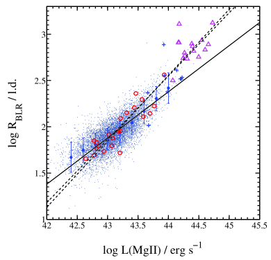
Figure 5: The relation between ${R_{\rm BLR}}$, estimated from $L_{5100}$, and $L\left({\rm Mg}{\textsc{ii}}\right)$, for several “H$\beta$$\times$Mg ii” sub-samples under study. Symbols are identical to Fig. 4. The solid black line represent the best-fit relation for the SDSS “H$\beta$$\times$Mg ii” sub-sample, which follows $\hbox{${R_{\rm BLR}}$}\propto L\left({\rm Mg}{\textsc{ii}}\right)^{0.5}$. The dashed lines alternative relations, derived by including the small, high-luminosity and high-redshift sample of M09. These relations follow $\hbox{${R_{\rm BLR}}$}\propto L\left({\rm Mg}{\textsc{ii}}\right)^{0.7}$. See the text and Table 2 for more details.

The line luminosity $L\left({\rm Mg}{\textsc{ii}}\right)$ can also be used to estimate ${R_{\rm BLR}}$. Such an approach may be used to overcome the difficulties in determining $L_{3000}$ in NIR spectra of high-redshift sources. The relation between ${R_{\rm BLR}}$, as determined from $L_{5100}$, and $L\left({\rm Mg}{\textsc{ii}}\right)$, is presented in Figure 5. The scatter in this relation is larger than that of the ${R_{\rm BLR}}$-$L_{3000}$ relation. In particular, the 2QZ “H$\beta$$\times$Mg ii” sub-sample shows considerable scatter and almost no correlation between ${R_{\rm BLR}}$ and $L\left({\rm Mg}{\textsc{ii}}\right)$, probably due to the low-quality of the data at this extreme redshift range (see §2.2). Fitting the data with a linear relation of the form

$$\log\hbox{${R_{\rm BLR}}$}=\alpha\,\log\left(\frac{L\left({\rm Mg}{\textsc{ii}}\right)}{10^{42}\,{\rm erg\,s}^{-1}}\right)\,+\beta\,\,$$ (8)

gives the values of $\alpha$ and $\beta$ presented in Table 2. We get $\alpha\left[L\left({\rm Mg}{\textsc{ii}}\right)\right]\simeq 0.5$ for the SDSS and 2QZ “H$\beta$$\times$Mg ii” sub-samples, but a considerably steeper slope (or a higher intercept) in the case we include the high-luminosity sources from the “small” samples. The scatter between the resulting (best-fit) estimates of ${R_{\rm BLR}}$ and those based on $L_{5100}$ (Eq. 2), for the SDSS and 2QZ sub-samples, is about 0.13 dex, only slightly higher than that of the ${R_{\rm BLR}}$-$L_{3000}$ relations. Despite the advantages of using this ${R_{\rm BLR}}$-$L\left({\rm Mg}{\textsc{ii}}\right)$ relation, we draw attention to the significant differences in the best-fit parameters that were derived from the different sub-samples, as well as by the two fitting methods, and caution that this relation is not as robust as the ${R_{\rm BLR}}$-$L_{3000}$ one. In addition, an accurate determination of $L\left({\rm Mg}{\textsc{ii}}\right)$ requires a reasonable determination of the Fe ii and Fe iii features adjacent to the Mg ii line, and thus still depends on the determination of the continuum.

6.3 The Width of the Mg ii $\lambda 2798$ Line

Our measure of FWHM(Mg ii) is different from the ones used in several earlier studies that measured the width of the total (doublet) profile. At large widths (${\rm FWHM}\left({\rm Mg}{\textsc{ii}}\right)\raisebox{-2.15277pt}{$\;\stackrel{{\scriptstyle>}}{{\sim}}\;$}4000\,{\rm km\,s}^{-1}$), the two widths are basically identical, since the width of the line is much larger than the separation between the two components. For relatively narrow lines (${\rm FWHM}\left({\rm Mg}{\textsc{ii}}\right)\lesssim 4000\,{\rm km\,s}^{-1}$) the two measures differ significantly, and ${\rm FWHM}\left({\rm Mg}{\textsc{ii}},{\rm single}\right)<{\rm FWHM}\left({\rm Mg}{\textsc{ii}},{\rm total}\right)$. For example, the typical profiles with (total) ${\rm FWHM}\left({\rm Mg}{\textsc{ii}}\right)\simeq 2000\,{\rm km\,s}^{-1}$ in our SDSS sample correspond to a single-component width of only $\sim 1500\,{\rm km\,s}^{-1}$. This implies that $M_{\rm BH}$ can be systematically overestimated by a factor of $\sim 1.8$ for such narrow-line objects. This issue is crucial for studies of sources with high accretion rates. To correct earlier results that used the entire profile, we suggest the following simple relation, which is based on a fit to the SDSS data:

$$FWHM\left({\rm Mg}{\textsc{ii}},{\rm single}\right)=1.01\times{\rm FWHM}\left({\rm Mg}{\textsc{ii}},{\rm total}\right)$$ (9)

$$-304\,{\rm km\,s}^{-1}.$$

We used this prescription to correct the relevant tabulated values of FWHM(Mg ii) published in earlier papers (see Table 1).

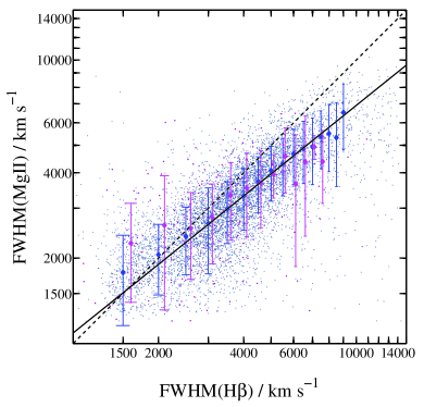
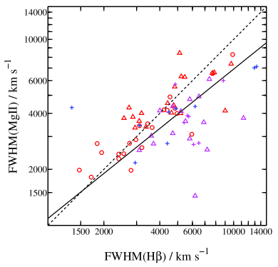
Figure 6: A comparison of FWHM(Mg ii) and FWHM(H$\beta$), for the large (left) and small (right) “H$\beta$$\times$Mg ii” sub-samples. In both panels, symbols are identical to Fig. 4, and the dashed lines represent the 1:1 relations. Solid lines represent the best-fit power-law relation, given in Eq. 10.

Several studies showed that FWHM(Mg ii) is very similar to FWHM(H$\beta$) (e.g. Shen et al., 2008, and references therein). This justifies the use of FWHM(Mg ii) as a tracer of virial BLR cloud motion. Indeed, the distribution of ${\rm FWHM}\left({\rm Mg}{\textsc{ii}}\right)/{\rm FWHM}\left({\rm H}\beta\right)$ for our SDSS “H$\beta$$\times$Mg ii” sub-sample peaks at -0.05 dex and the standard deviation is 0.15 dex. A similar comparison of the IPV line widths results in an almost identical distribution. In order to further test this issue, we present in Figure 6 a direct comparison between FWHM(Mg ii) and FWHM(H$\beta$), for all the “H$\beta$$\times$Mg ii” sub-samples. As expected, there is a strong correlation between the widths of the two lines. However, in most of the cases with ${\rm FWHM}\left({\rm H}\beta\right)\raisebox{-2.15277pt}{$\;\stackrel{{\scriptstyle>}}{{\sim}}\;$}4000\,{\rm km\,s}^{-1}$, the Mg ii line is narrower. This trend is also reflected in the binned data shown in Fig. 6. For example, for sources with ${\rm FWHM}\left({\rm H}\beta\right)\simeq 9000\,{\rm km\,s}^{-1}$, the typical value for the Mg ii line is merely ${\rm FWHM}\left({\rm Mg}{\textsc{ii}}\right)\simeq 6000\,{\rm km\,s}^{-1}$. We find that the best-fit relation between these line widths is

$$\log\,{\rm FWHM}\left({\rm Mg}{\textsc{ii}}\right)=\left(0.803\pm 0.007\right)\log{\rm FWHM}\left({\rm H}\beta\right)\,$$ (10)

$$+\,\left(0.628\pm 0.027\right)\,,$$

based on the BCES bisector. This relation is also shown in Fig. 6. Our result is in excellent agreement, both in terms of slope and intercept, with that of Wang et al. (2009), which is based on a subset of our SDSS “H$\beta$$\times$Mg ii” sub-sample (about 10% of the sources; see §2.1). The general trend we find between FWHM(Mg ii) and FWHM(H$\beta$) is captured, in essence, by the statistical correction factors suggested by Onken & Kollmeier (2008), which are useful for large samples. However, it is not at all clear whether the fit reflects a real, global trend. The alternative is that ${\rm FWHM}\left({\rm Mg}{\textsc{ii}}\right)\simeq{\rm FWHM}\left({\rm H}\beta\right)$ up to $\sim 6000\,{\rm km\,s}^{-1}$, beyond which there are some differences in the mean location of the strongest line emitting gas.

6.4 Determination of $M_{\rm BH}\left({\rm Mg}{\textsc{ii}}\right)$

For each source in the “H$\beta$$\times$Mg ii” sub-samples we calculated an “empirical scaling factor”:

$$\mu\left({\rm Mg}{\textsc{ii}}\right)\equiv\frac{1}{G}\,\hbox{${R_{\rm BLR}}$}\left(L_{3000}\right)\,{\rm FWHM}\left({\rm Mg}{\textsc{ii}}\right)^{2}\,,$$ (11)

where $\hbox{${R_{\rm BLR}}$}\left(L_{3000}\right)$ is calculated through Eq. 7. In Figure 7 we show the distribution of the relevant normalization factor, defined as $f\left({\rm Mg}{\textsc{ii}}\right)=M_{\rm BH}\left({\rm H}\beta\right)/\mu\left({\rm Mg}{\textsc{ii}}\right)$, for the SDSS “H$\beta$$\times$Mg ii” sub-sample. The distribution has a clear peak at a median (mean) value is $f\left({\rm Mg}{\textsc{ii}}\right)=1.33$ (1.42), and a standard deviation of 0.32 dex. This is in agreement with the expected value of $f\left({\rm Mg}{\textsc{ii}}\right)=1$. For comparison, the McLure & Dunlop (2004) $M_{\rm BH}$ estimator was derived assuming $f\left({\rm Mg}{\textsc{ii}}\right)=0.89$. We further investigated whether $f\left({\rm Mg}{\textsc{ii}}\right)$ depends on other observables, such as source luminosity, SED shape or EW(Mg ii). However, we find no significant correlations of this type. The only exception, a marginal anti-correlation with $L/L_{\rm Edd}$ (see §4.2) is most probably driven by the strong dependence of both $L/L_{\rm Edd}$ and $f\left({\rm Mg}{\textsc{ii}}\right)$ on FWHM(H$\beta$). In addition, the small scatter in the $\hbox{${R_{\rm BLR}}$}-L_{3000}$ relation, in comparison with that of the ${\rm FWHM}\left({\rm H}\beta\right)-{\rm FWHM}\left({\rm Mg}{\textsc{ii}}\right)$ relation, suggests that the range of derived $f\left({\rm Mg}{\textsc{ii}}\right)$ values is driven solely by the scatter in ${\rm FWHM}\left({\rm H}\beta\right)/{\rm FWHM}\left({\rm Mg}{\textsc{ii}}\right)$. This is supported by the fact that we find no correlation between $f\left({\rm Mg}{\textsc{ii}}\right)$ and $L_{3000}/L_{5100}$ while the significant correlation with ${\rm FWHM}\left({\rm H}\beta\right)/{\rm FWHM}\left({\rm Mg}{\textsc{ii}}\right)$ (not shown here) tightly follows a power-law with the expected slope of about 2.

Next, we combine our best-fit $\hbox{${R_{\rm BLR}}$}-L_{3000}$ relation (Eq. 7) with FWHM(Mg ii) and the median value of $f\left({\rm Mg}{\textsc{ii}}\right)$ to obtain the final form of the Mg ii-based $M_{\rm BH}$ estimator,

$$M_{\rm BH}=5.6\times 10^{6}\left[\frac{L_{3000}}{10^{44}\,{\rm erg\,s}^{-1}}\right]^{0.62}\left[\frac{{\rm FWHM}({\rm Mg}{\textsc{ii}})}{10^{3}\,{\rm km\,s}^{-1}\,}\right]^{2}\,\,M_{\odot}\ .$$ (12)

This estimator differs from the one given in MD04 in its overall normalization, which is higher by a factor of about 1.75 than the MD04 one. Thus, we find that the MD04 $M_{\rm BH}$ estimator causes an underestimation of $M_{\rm BH}$ by $\sim 0.25$ dex. This result is consistent with the findings of Shen et al. (2011), where the slope of the $\hbox{${R_{\rm BLR}}$}-L_{3000}$ relation was forced to be 0.62. Naturally, the choice of a different $\hbox{${R_{\rm BLR}}$}-L_{3000}$ relation, according to the parameters listed in Table 2, would result in subtle luminosity-dependent differences between our $M_{\rm BH}$ estimates and those of MD04. We repeated the above steps for several other choices of parameters ($\alpha$ and $\beta$ in Eq. 6), and list in Table 2 the resulting scaling of the final $M_{\rm BH}$ estimator (i.e. the equivalents of 5.6 in Eq. 12 above). Thus, one can use a different $L_{3000}$-based virial $M_{\rm BH}$ estimator, fully described by $\alpha$ and $M_{0}$ in Table 2, according to the required luminosity range (see discussion in §6.1).

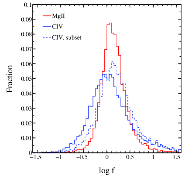
Figure 7: The distributions of empirically derived normalization factors $\left(f\right)$, for different emission lines and sub-samples. The solid red line represents the distribution of $f\left({\rm Mg}{\textsc{ii}}\right)$ (see §6.4), for the SDSS “H$\beta$$\times$Mg ii” sub-sample. The solid blue line represents the distribution of $f\left({\rm C}\,\textsc{iv}\right)$ for the entire SDSS “Mg ii$\times$C iv” sub-sample, while the dashed blue line represents the subset of sources which show $|v_{\rm off}({\rm C}\,\textsc{iv})|<500\,\,{\rm km\,s}^{-1}$.

To evaluate the improvement we obtained in estimating $M_{\rm BH}$(Mg ii), we compare in Figure 8 the masses obtained with the H$\beta$ (following Eq. 3) and the MD04 methods, for all the “H$\beta$$\times$Mg ii” sub-samples. Clearly, there is a systematic offset between the two estimators, in the sense that $M_{\rm BH}$(Mg ii,MD04) is typically lower than $M_{\rm BH}$(H$\beta$). The median offset within the SDSS “H$\beta$$\times$Mg ii” sub-sample is, indeed, $\sim 0.25$ dex. In Figure 9 we preform a similar comparison, but this time using the new Mg ii-based $M_{\rm BH}$ estimates (Eq. 12). The systematic shift seen in Fig. 8, particularly at the high mass end, has completely disappeared. The median difference between the two estimates is negligible, although the scatter (standard deviation of residuals) remains about 0.32 dex.

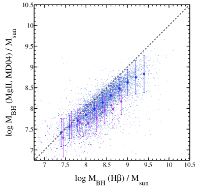
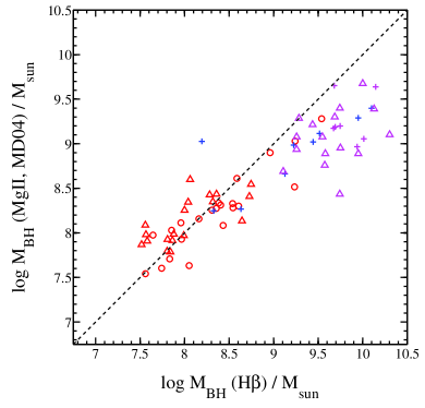
Figure 8: A comparison of estimates of $M_{\rm BH}$ based on the H$\beta$ line and the McLure & Dunlop (2004) prescription, for the large (left) and small (right) “H$\beta$$\times$Mg ii” sub-samples. In both panels, symbols are identical to Fig. 4, and the dashed lines represent the the 1:1 relations.

Several studies suggested to use $M_{\rm BH}$ estimators where the exponent of the velocity term differs from 2 (e.g., Greene & Ho, 2005; Wang et al., 2009). Like any additional degree of freedom, it is expected that this approach may reduce the scatter between H$\beta$- and Mg ii-based estimates of $M_{\rm BH}$. The usage of this empirical approach abandons the fundamental assumption of virialized BLR dynamics, which is the basis for all mass determinations considered here. For the sake of completeness, we derived a relation by combining Eqs 7 and 10 and minimizing the systematic offset with respect to the the H$\beta$-based $M_{\rm BH}$ estimators. This process resulted in the relation $M_{\rm BH}=3.62\times 10^{6}\left[\frac{L_{3000}}{10^{44}\,{\rm erg\,s}^{-1}}\right]^{0.62}\left[\frac{{\rm FWHM}({\rm Mg}{\textsc{ii}})}{10^{3}\,{\rm km\,s}^{-1}\,}\right]^{2.5}\,\,M_{\odot}$ . The scatter between this estimator and the one based on H$\beta$, for the SDSS “H$\beta$$\times$Mg ii” sub-sample, is of 0.34 dex, almost identical to the one obtained following Eq. 12 above. Since this relation departs from the simple virial assumption, we chose not to use in what follows.

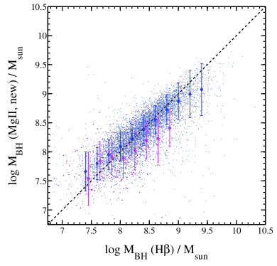
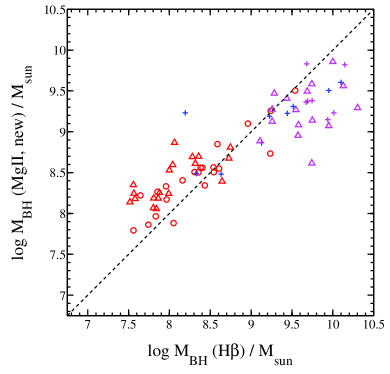
Figure 9: A comparison of H$\beta$-based estimates of $M_{\rm BH}$, and the new calibration of a Mg ii-based $M_{\rm BH}$ estimator, for the large (left) and small (right) “H$\beta$$\times$Mg ii” sub-samples. The H$\beta$- and Mg ii-based $M_{\rm BH}$ estimates are obtained through Eqs. 3 and 12, respectively. In both panels, symbols are identical to Fig. 4, and the dashed lines represent the the 1:1 relations.

$M_{\rm BH}$ can also be obtained by using the ${R_{\rm BLR}}$-$L\left({\rm Mg}{\textsc{ii}}\right)$ relation presented in §6.2. We have repeated the steps described above, assuming $\left(\hbox{${R_{\rm BLR}}$}/\rm{l.d.}\right)=24\left(L\left({\rm Mg}{\textsc{ii}}\right)/10^{42}\,{\rm erg\,s}^{-1}\right)^{0.5}$ (see Table 2), and obtained

$$M_{\rm BH}=6.79\times 10^{6}\left[\frac{L\left({\rm Mg}{\textsc{ii}}\right)}{10^{42}\,{\rm erg\,s}^{-1}}\right]^{0.5}\left[\frac{{\rm FWHM}({\rm Mg}{\textsc{ii}})}{10^{3}\,{\rm km\,s}^{-1}\,}\right]^{2}\,\,M_{\odot}\ .$$ (13)

$M_{\rm BH}$ estimates based on this relation are also consistent with those based on H$\beta$, and the scatter for the SDSS “H$\beta$$\times$Mg ii” sub-sample is of 0.33 dex, indistinguishable from the one achieved by using $L_{3000}$. We note that the Mg ii line presents a clear “Baldwin effect”, i.e. an anti-correlation between EW(Mg ii) and $L_{3000}$ (e.g. Baldwin, 1977, BL05). Therefore, the usage of $L\left({\rm Mg}{\textsc{ii}}\right)$ probably incorporates some other, yet-unknown properties of the BLR.

We tested the consistency of our improved $L_{3000}$-based determinations of $L/L_{\rm Edd}$ with those based on $L_{5100}$ (and H$\beta$). For this, we calculated $L/L_{\rm Edd}$ for the SDSS “H$\beta$$\times$Mg ii” sub-sample based on the two available approaches: either using the bolometric corrections given by Eq. 5 and $M_{\rm BH}$ estimates given by Eq. 12, or using the bolometric corrections of Marconi et al. (2004) and $M_{\rm BH}$ estimates given by Eq. 3. In all cases we assume $L_{\rm Edd}=1.5\times 10^{38}\left(M_{\rm BH}/M_{\odot}\right)\,{\rm erg\,s}^{-1}$, appropriate for solar metallicity gas. The comparison of the two estimates of $L/L_{\rm Edd}$ clearly shows that the two agree well, with a scatter of about 0.31 dex, and negligible systematic difference. On the other hand, using the bolometric correction of Richards et al. (2006a, 5.15) and the MD04 estimates of $M_{\rm BH}$ results in a systematic overestimation of $L/L_{\rm Edd}$ by a factor of about 2.2.

7 C iv $\lambda 1549$-based estimates of $M_{\rm BH}$

As discussed in §5, under the virial assumption, and the known ratio of FWHM(C iv)/FWHM(H$\beta$) in a small number of sources with RM-based ${R_{\rm BLR}}$ measurements, it is possible to use a reliable estimator for the size of the C iv-emitting region (Eq. 4) to calibrate a C iv-based estimator for $M_{\rm BH}$, by combining ${R_{\rm BLR}}$($L_{1450}$), FWHM(C iv) and a known $f$-factor ($f=1$ in our case). Since for the samples where ${R_{\rm BLR}}$(C iv) is directly measured it is smaller than ${R_{\rm BLR}}$(H$\beta$), by a factor of $\sim$3.7, we expect $\left({\rm FWHM}\left({\rm C}\,\textsc{iv}\right)/{\rm FWHM}\left({\rm H}\beta\right)\right)\simeq\sqrt{3.7}=1.9$. In what follows, we address the different ingredients of a virial C iv-based estimator, and show that for a large number of the type-I AGN studied here the C iv measurements are not consistent with the virial assumption.

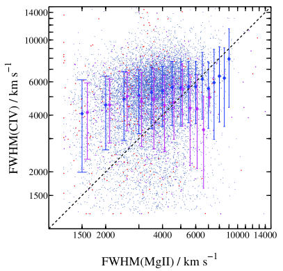
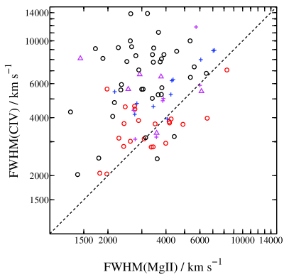
Figure 10: A comparison of FWHM(C iv) and FWHM(Mg ii) for the different “Mg ii$\times$C iv” sub-samples. Left - large samples: blue, magenta and red points represent the SDSS, 2QZ and 2SLAQ , respectively. Larger symbols and error bars represent the binned data and the corresponding scatter (standard deviations). Right - small samples: black circles represent the T11 sample (at $z\simeq 4.8$), while all other symbols are identical to previous figures. In both panels, the dashed lines represent the the 1:1 relations.

Figures 10 and 11 compare FWHM(C iv) with FWHM(Mg ii) and FWHM(H$\beta$), respectively. The scatter in both figures is much larger than the scatter in the Mg ii-H$\beta$ comparison diagram (Fig. 6), and the line widths do not follow each other. In practical terms, for any observed (single) value of FWHM(C iv), the corresponding values of FWHM(H$\beta$) covers almost the entire range of $\sim 2,000-10,000\,{\rm km\,s}^{-1}$, in contrast with the value expected from the assumption of virialized motion and an identical $f$. We verified that alternative measures of the line width, such as the IPV, do not reduce the scatter or present any more significant relations between the different lines. Most importantly, a significant fraction of the sources under study ($\sim 45\%$) exhibit ${\rm FWHM}\left({\rm C}\,\textsc{iv}\right)\leq{\rm FWHM}\left({\rm H}\beta\right)$ (Fig. 11), and 26% of the sources in the SDSS, 2QZ & 2SLAQ “Mg ii$\times$C iv” sub-samples have ${\rm FWHM}\left({\rm C}\,\textsc{iv}\right)\leq{\rm FWHM}\left({\rm Mg}{\textsc{ii}}\right)$ (Fig. 10), in contrast to the expectations of the virial method. The large scatter, and the lack of any correlation between FWHM(C iv) and either FWHM(H$\beta$) or FWHM(Mg ii), were identified in several earlier studies of local (e.g. Corbin & Boroson, 1996, BL05), intermediate- (e.g., S08, F08) and high-redshift (S04, N07, T11) samples. We note that the high fraction of sources where FWHM(C iv) seems to defy the expectations is not due to a specific population of narrow-line sources (i.e., NLSy1s), and/or low-quality UV spectra, as was suggested by Vestergaard & Peterson (2006). In particular, we find that 55% of the “H$\beta$$\times$C iv” sources with ${\rm FWHM}\left({\rm H}\beta\right)>3000\,{\rm km\,s}^{-1}$ (i.e., 88 out of 155 broad-line sources) present ${\rm FWHM}\left({\rm C}\,\textsc{iv}\right)\leq{\rm FWHM}\left({\rm H}\beta\right)$. In addition, 51% of the sources in the N07+S04, D09 & M09 samples (33 out of 65 sources), where the C iv line was measured in high-quality optical spectra, also show ${\rm FWHM}\left({\rm C}\,\textsc{iv}\right)\leq{\rm FWHM}\left({\rm H}\beta\right)$.

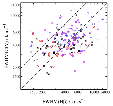
Figure 11: A comparison of FWHM(C iv) and FWHM(H$\beta$) for all the “H$\beta$$\times$C iv” sub-samples. Symbols are identical to Fig. 1. The dashed line represents the 1:1 relation, while the dot-dashed line represents ${\rm FWHM}\left({\rm C}\,\textsc{iv}\right)=\sqrt{3.7}{\rm FWHM}\left({\rm H}\beta\right)$, as predicted by the virial assumption (see §5 for details). Note the large fraction of sources with ${\rm FWHM}\left({\rm C}\,\textsc{iv}\right)\lesssim{\rm FWHM}\left({\rm H}\beta\right)$, in sharp contrast with the virial assumption, and the very large scatter.

To further understand the large scatter in Figs. 10 and 11, we tried to look for correlations between either ${\rm FWHM}\left({\rm C}\,\textsc{iv}\right)/{\rm FWHM}\left({\rm Mg}{\textsc{ii}}\right)$ or ${\rm FWHM}\left({\rm C}\,\textsc{iv}\right)/{\rm FWHM}\left({\rm H}\beta\right)$ and other AGN properties. The different panels in Figure 12 compare ${\rm FWHM}\left({\rm C}\,\textsc{iv}\right)/{\rm FWHM}\left({\rm Mg}{\textsc{ii}}\right)$ with $L_{\rm bol}$, $M_{\rm BH}$, $L/L_{\rm Edd}$, and the shape of the optical-UV SED, $\alpha_{\nu,{\rm UVO}}$. In this comparison, $L_{\rm bol}$, $M_{\rm BH}$, $L/L_{\rm Edd}$ and $\alpha_{\nu,{\rm UVO}}$ were calculated from H$\beta$-related observables whenever possible (i.e. the M09, Mc08 and Sh07 samples), and using Eq. 3 and the Marconi et al. (2004) bolometric corrections. In all other cases these quantities were calculated from the Mg ii-related observables and Eqs. 12 & 5. The shape of the SED is calculated following $\alpha_{\nu,{\rm UVO}}=-\left[\log\left(L_{5100}/L_{1450}\right)/\left(5100/1450\right)\right]-1$, or $\alpha_{\nu,{\rm UVO}}=-\left[\log\left(L_{3000}/L_{1450}\right)/\left(3000/1450\right)\right]-1$, for the “Mg ii$\times$C iv” sub-samples that lack $L_{5100}$ measurements. Most panels show considerable scatter, and a lack of any significant correlations. Although the SDSS sub-sample shows some systematic trends of ${\rm FWHM}\left({\rm C}\,\textsc{iv}\right)/{\rm FWHM}\left({\rm Mg}{\textsc{ii}}\right)$ with $M_{\rm BH}$ and $L/L_{\rm Edd}$ (see also Wang et al., 2011), these trends completely disappear once the smaller samples are taken into account. These trends are thus a result of the very limited range in luminosity of the SDSS “Mg ii$\times$C iv” sub-sample, and the dependence of $M_{\rm BH}$ (and $L/L_{\rm Edd}$) on FWHM(Mg ii). In particular, we draw attention to the lack of a significant (anti-)correlation between ${\rm FWHM}\left({\rm C}\,\textsc{iv}\right)/{\rm FWHM}\left({\rm Mg}{\textsc{ii}}\right)$ and $\alpha_{\nu,{\rm UVO}}$. Such an anti-correlation is expected due to the similar forms of the $\hbox{${R_{\rm BLR}}$}-L$ relations (Eqs. 2 & 4), the uniformity of UV-optical SEDs (§4.1), and the virial assumption. We will return to this point below. The different panels in Fig. 12 also demonstrate that the population of sources that do not comply with the basic expectations (i.e. sources with ${\rm FWHM}\left({\rm C}\,\textsc{iv}\right)<{\rm FWHM}\left({\rm Mg}{\textsc{ii}}\right)$) cannot be distinguished from the general population.

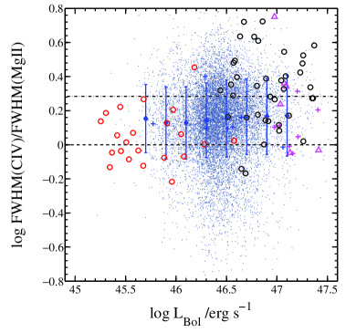
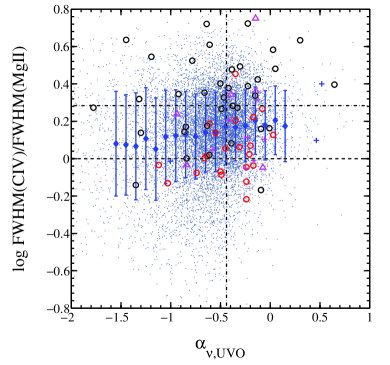
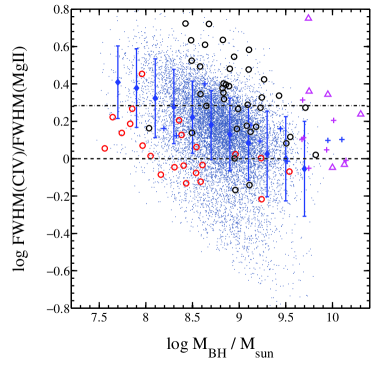
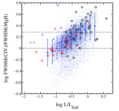
Figure 12: The relations between the difference in the Mg ii and C iv line width, $\log\left({\rm FWHM}\left({\rm C}\,\textsc{iv}\right)/{\rm FWHM}\left({\rm Mg}{\textsc{ii}}\right)\right)$, and several AGN properties (left to right, top to bottom): $L_{\rm bol}$, $\alpha_{\nu,{\rm UVO}}$, $M_{\rm BH}$ and $L/L_{\rm Edd}$. In all panels, small blue dots represent the SDSS “Mg ii$\times$C iv” sub-sample, while larger blue diamond symbols and error bars represent the binned data and the corresponding scatter (standard deviations). Symbols for several of the small samples are identical to previous figures. The dashed lines represent ${\rm FWHM}\left({\rm C}\,\textsc{iv}\right)={\rm FWHM}\left({\rm Mg}{\textsc{ii}}\right)$, while the dot-dashed lines represent ${\rm FWHM}\left({\rm C}\,\textsc{iv}\right)=\sqrt{3.7}{\rm FWHM}\left({\rm Mg}{\textsc{ii}}\right)$, as expected from the virial assumption. Note the large scatter in all panels, as well as the lack of significant correlations among samples of different luminosities. The apparent trends within the SDSS “Mg ii$\times$C iv”sub-sample (in the lower panels) are due to its limited luminosity range and the dependence of $M_{\rm BH}$ and $L/L_{\rm Edd}$ on FWHM(Mg ii).

An alternative way to examine this issue is to drop the assumption that $f$ is the same for all lines, and consider empirical estimates of the $f$-factors associated with a C iv-based estimator of $M_{\rm BH}$. This can be done by combining the $\hbox{${R_{\rm BLR}}$}-L_{1450}$ relation (given by Kaspi et al., 2007, Eq. 4) and FWHM(C iv), for all the “H$\beta$$\times$C iv” and “Mg ii$\times$C iv” sub-samples, into a “virial product” of the form

$$\mu\left({\rm C}\,\textsc{iv}\right)=2.09\times 10^{8}\left[\frac{L_{1450}}{10^{46}\,{\rm erg\,s}^{-1}}\right]^{0.55}\left[\frac{{\rm FWHM}\left({\rm C}\,\textsc{iv}\right)}{10^{3}\,{\rm km\,s}^{-1}}\right]^{2}\,\,M_{\odot}\,.$$ (14)

We can then calculate the C iv-related $f$-factors ($f\left({\rm C}\,\textsc{iv}\right)\equiv M_{\rm BH}/\mu\left({\rm C}\,\textsc{iv}\right)$), where $M_{\rm BH}$ is determined either from $L_{5100}$ & FWHM(H$\beta$) (Eq. 3) or $L_{3000}$ & FWHM(Mg ii) (Eq. 12). As mentioned above, we expect $f\left({\rm C}\,\textsc{iv}\right)=f\left({\rm H}\beta\right)=1$.

The distribution of $f\left({\rm C}\,\textsc{iv}\right)$ for the SDSS “Mg ii$\times$C iv” sub-sample is shown in Figure 7. It shows a very broad distribution with a peak at about $f\left({\rm C}\,\textsc{iv}\right)=1.1$, in agreement with the expected value. Thus, formally, the usage of $L_{1450}$ and FWHM(C iv) can reproduce the correct typical $M_{\rm BH}$ for a large sample of sources. The recent study of Croom (2011) showed that, indeed, for large samples with narrow ranges of redshift and luminosities, the typical (average) $M_{\rm BH}$ can be determined solely based on the distribution of luminosities, regardless of FWHM. However, the scatter in $f\left({\rm C}\,\textsc{iv}\right)$ (the standard deviation), for the SDSS “Mg ii$\times$C iv” sub-sample, is about 0.46 dex. Moreover, 25% of the sources show $f\left({\rm C}\,\textsc{iv}\right)>2.1$ and an additional 25% show $f\left({\rm C}\,\textsc{iv}\right)<0.6$. This practically prohibits the usage of a single scaling factor to determine $M_{\rm BH}$ in individual sources. Since the scatter in $L_{1450}/L_{3000}$ and $L_{1450}/L_{5100}$ is rather small (see §4.1), and since the slopes in the different $\hbox{${R_{\rm BLR}}$}-L$ relations are similar, most of the scatter in $f\left({\rm C}\,\textsc{iv}\right)$ is probably due to the scatter in ${\rm FWHM}\left({\rm C}\,\textsc{iv}\right)/{\rm FWHM}\left({\rm Mg}{\textsc{ii}}\right)$ and ${\rm FWHM}\left({\rm C}\,\textsc{iv}\right)/{\rm FWHM}\left({\rm H}\beta\right)$. We investigate this point further by plotting, in Figure 13, the $f$-factor against several observed properties. The large scatter, and lack of correlation among samples of different luminosities, is evident in all the panels, and in particular in the comparison with $\alpha_{\nu,{\rm UVO}}$. In contrast, a comparison of $f\left({\rm C}\,\textsc{iv}\right)$ with ${\rm FWHM}\left({\rm C}\,\textsc{iv}\right)/{\rm FWHM}\left({\rm Mg}{\textsc{ii}}\right)$ exhibits a very prominent correlation, which closely follows a $f\left({\rm C}\,\textsc{iv}\right)\propto\left({\rm FWHM}\left({\rm C}\,\textsc{iv}\right)/{\rm FWHM}\left({\rm Mg}{\textsc{ii}}\right)\right)^{2}$ trend. This clearly demonstrates that the main source for differences between the different virial $M_{\rm BH}$ estimators are the large and unsystematic differences between FWHM(C iv) and FWHM(Mg ii) (or other velocity measures).

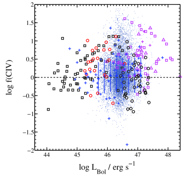
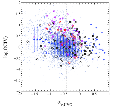
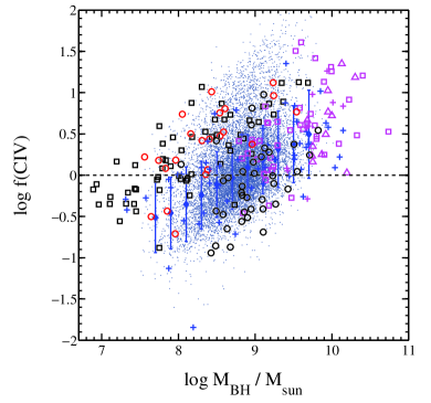
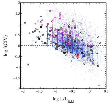
Figure 13: The relations between the scaling factor $f\left({\rm C}\,\textsc{iv}\right)$ and several AGN properties (left to right, top to bottom): $L_{\rm bol}$, $\alpha_{\nu,{\rm UVO}}$, $M_{\rm BH}$ and $L/L_{\rm Edd}$. Symbols are identical to previous figures. The dashed lines mark $f\left({\rm C}\,\textsc{iv}\right)=1$, as expected from the virial assumption and $f\left({\rm H}\beta\right)=1$ . Note the large scatter in all panels, as well as the lack of significant correlations among samples of different luminosities. Here too, the apparent trends within the SDSS “Mg ii$\times$C iv” sub-sample (in the lower panels) are due to its limited luminosity range and the dependence of $M_{\rm BH}$ and $L/L_{\rm Edd}$ on FWHM(Mg ii).

The recent study by Assef et al. (2011) presented detailed measurements of H$\beta$ and C iv for 12 lensed QSOs at $z=1.5-3.6$, drawn from the CASTLES survey. These authors suggest that the differences between $M_{\rm BH}$(H$\beta$) and $M_{\rm BH}$(C iv) (estimated using the calibration of Vestergaard & Peterson, 2006) are mainly driven by the shape of the UV-optical SED (i.e., $L_{1450}$/$L_{5100}$), and provide empirical correction terms to account for these differences. As noted in §4.1, the (small) sample of Assef et al. (2011) includes heavily reddened sources, with about a half of their sources having $L_{5100}>L_{1450}$ (corresponding to $\alpha_{\nu,{\rm UVO}}<-1$). Less than 15% of our SDSS sources show such red SEDs. The corrections provided by Assef et al. (2011) thus minimize the effect of the SED shape, or reddening, on $M_{\rm BH}$ estimates. However, as we showed above, the main driver for the discrepancy between $M_{\rm BH}$(H$\beta$) and $M_{\rm BH}$(C iv) is most probably related to FWHM(C iv), and not to the SED shape. Indeed, almost half of sources in the Assef et al. (2011) sample have ${\rm FWHM}\left({\rm C}\,\textsc{iv}\right)\raisebox{-2.15277pt}{$\;\stackrel{{\scriptstyle<}}{{\sim}}\;$}{\rm FWHM}\left({\rm H}\beta\right)$, in contrast with the virial assumption, and in agreement with the fraction of such sources in our “H$\beta$$\times$C iv” sub-samples. Moreover, Assef et al. (2011) report a large scatter between FWHM(C iv) and FWHM(H$\beta$), similarly to our findings. We also note that the usage of correction terms which are based on $L_{5100}$ (or FWHM(H$\beta$)) is impractical for large samples of $z\raisebox{-2.15277pt}{$\;\stackrel{{\scriptstyle>}}{{\sim}}\;$}0.8$ sources. On the other hand, if the H$\beta$ line for such sources is available (through NIR spectroscopy), it can be used to determine $M_{\rm BH}$ directly (e.g., by using Eq. 3), and we see no point in using it solely to correct systematics in $M_{\rm BH}$(C iv).

Figs. 12 and 13 demonstrate that the discrepancies associated with a C iv-based virial product cannot be accounted for even if other basic AGN properties are known. Moreover, some of these properties cannot be reliably determined a-priori, given a single spectrum that contains only the C iv line. We therefore tested the possibility of correcting the discrepancy described above by using only C iv-related observables, namely the shift ($v_{\rm off}$[C iv]) of the line center and the equivalent width of the line (EW[C iv]). Previous studies suggested that the large blue-shifts often observed in C iv indicate that the emission originates from non-virialized gas motion (e.g., BL05, Richards et al., 2011). Such a scenario may explain why a simple virial product (Eq. 14) fails to scale with $M_{\rm BH}$. A trend with EW(C iv) might be expected if, for example, there was a common origin for the difference in FWHM and the well-known Baldwin Effect.

We first verified that there is no clear trend of neither ${\rm FWHM}\left({\rm C}\,\textsc{iv}\right)/{\rm FWHM}\left({\rm Mg}{\textsc{ii}}\right)$ nor $f\left({\rm C}\,\textsc{iv}\right)$ with EW(C iv). In particular, the population of sources with ${\rm FWHM}\left({\rm C}\,\textsc{iv}\right)<{\rm FWHM}\left({\rm Mg}{\textsc{ii}}\right)$ cannot be distinguished from the rest of the sources based on their EW(C iv). Next, We calculated the shifts of the C iv line relative to the Mg ii for the “Mg ii$\times$C iv” sub-samples under study. We assumed that the rest-frame center of the Mg ii doublet is at 2799.11Å, and that the C iv profile is centered at 1549.48Å. Our fitting procedures calculate the observed line centers as the peaks of the entire best-fit BLR profile. Figure 14 presents the resulting $v_{\rm off}$(C iv) against ${\rm FWHM}\left({\rm C}\,\textsc{iv}\right)/{\rm FWHM}\left({\rm Mg}{\textsc{ii}}\right)$. As is the case in Fig. 12, the scatter is very large and covers more than a factor of 5 in ${\rm FWHM}\left({\rm C}\,\textsc{iv}\right)/{\rm FWHM}\left({\rm Mg}{\textsc{ii}}\right)$. However, there appears to be a clear trend of an increasing ${\rm FWHM}\left({\rm C}\,\textsc{iv}\right)/{\rm FWHM}\left({\rm Mg}{\textsc{ii}}\right)$ with increasing C iv blue-shift (negative velocities).

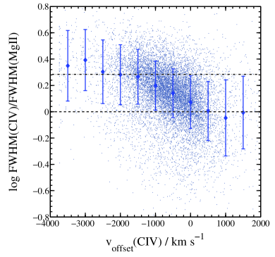
Figure 14: The relation between the difference in the Mg ii and C iv line width, and the offset of the C iv line with respect to the Mg ii line, for the SDSS “Mg ii$\times$C iv” sub-sample. Larger symbols and error bars represent the binned data and the corresponding scatter (standard deviations). The dashed line represents ${\rm FWHM}\left({\rm C}\,\textsc{iv}\right)={\rm FWHM}\left({\rm Mg}{\textsc{ii}}\right)$, while the dot-dashed line represents ${\rm FWHM}\left({\rm C}\,\textsc{iv}\right)=\sqrt{3.7}{\rm FWHM}\left({\rm Mg}{\textsc{ii}}\right)$, as expected from the virial assumption.

Figure 14 draws attention to two particular types of sources which may, in principle, be used to overcome the problems associated with FWHM(C iv). First, C iv lines in sources with small offsets may be dominated by virialized gas. To test this, we selected a subset of about 4500 sources from the SDSS “Mg ii$\times$C iv” sub-sample that have $|v_{\rm off}({\rm C}\,\textsc{iv})|<500\,{\rm km\,s}^{-1}$. The distribution of $f\left({\rm C}\,\textsc{iv}\right)$ for this subset is shown in Fig. 7. Clearly, the large scatter in ${\rm FWHM}\left({\rm C}\,\textsc{iv}\right)/{\rm FWHM}\left({\rm Mg}{\textsc{ii}}\right)$, of more than 0.2 dex, propagated to the virial products of these sources. Moreover, the typical $f\left({\rm C}\,\textsc{iv}\right)$ for this subset is 1.49 - considerably higher than the expected value (of unity). Second, sources with blueshifts of about $1500-2500\,{\rm km\,s}^{-1}$ appear to match the expected value of ${\rm FWHM}\left({\rm C}\,\textsc{iv}\right)/{\rm FWHM}\left({\rm Mg}{\textsc{ii}}\right)\simeq 1.9$. Here too, the scatter in ${\rm FWHM}\left({\rm C}\,\textsc{iv}\right)/{\rm FWHM}\left({\rm Mg}{\textsc{ii}}\right)$ for the relevant sources is larger than 0.2 dex, and the scatter in $f\left({\rm C}\,\textsc{iv}\right)$ is 0.5 dex. Moreover, there is no physical motivation for focusing on lines with such particular offset velocities, which are probably produced by non-virialized gas. Thus, C iv cannot be used to precisely estimate $M_{\rm BH}$ even for these specific sources. We also note the great difficulty in robustly determining $v_{\rm off}$(C iv) in optical spectra of high redshift sources, where the systemic redshift determination heavily relies on a few UV lines, including C iv itself and the complex, often partially absorbed Ly$\alpha$ spectral region.

We conclude that the C iv line is an unreliable probe of the kinematics of the BLR gas. There is a significant population of type-I AGN, indistinguishable from the general population, for which the width of the C iv line contradicts the basic virial expectation. A single-epoch $M_{\rm BH}$ estimator which relies on the width of the C iv line provides results that deviate by $\pm$0.46 dex from the more reliable H$\beta$-based estimator. This scatter is due to $f\left({\rm C}\,\textsc{iv}\right)$ only and was estimated assuming a constant $f\left({\rm H}\beta\right)$ and negligible uncertainties in the $\hbox{${R_{\rm BLR}}$}-L$ relations and in the measurements of all relevant observables. The uncertainty in individual C iv-based estimates of $M_{\rm BH}$ can be considerably larger (see Woo et al. (2010) for the case of $f\left[{\rm H}\beta\right]$).

8 Discussion and Conclusions

The reliable estimators of $M_{\rm BH}$ and $L/L_{\rm Edd}$ obtained in the present work should enable us to examine the observed distributions of these quantities, and their evolution over cosmic epochs. However, since both $M_{\rm BH}$ and $L/L_{\rm Edd}$ depend on the source luminosity, their observed distributions, at any given redshift, would suffer from selection effects due to the flux limit of the respective survey. The treatment of this issue requires the application of dedicated statistical methods (e.g., Kelly et al., 2010, NT07), which is beyond the scope of this paper. We thus only briefly present here the preliminary results that concern the upper envelope of the $M_{\rm BH}$ and $L/L_{\rm Edd}$ distributions, and defer the full analysis of the observed SMBH evolution to a forthcoming paper.

We apply the H$\beta$- and Mg ii-based prescriptions to all the samples listed in Table 1. For sources with reliable H$\beta$ measurements (mainly SDSS sources at $z\leq 0.75$), the bolometric luminosities are estimated using the Marconi et al. (2004) corrections and $M_{\rm BH}$ is calculated through Eq. 3. For sources with reliable Mg ii measurements (mainly SDSS sources at $0.75\raisebox{-2.15277pt}{$\;\stackrel{{\scriptstyle<}}{{\sim}}\;$}z\raisebox{-2.15277pt}{$\;\stackrel{{\scriptstyle<}}{{\sim}}\;$}2$) we use the bolometric corrections given by Eq. 5, while $M_{\rm BH}$ is calculated by Eq. 12. In all cases where more than one line is observed, we prefer H$\beta$-based measurements on other measurements.

Figure 15 describes the evolution of $M_{\rm BH}$ with the age of the Universe, for the SDSS, 2QZ & 2SLAQ samples (at $z\raisebox{-2.15277pt}{$\;\stackrel{{\scriptstyle<}}{{\sim}}\;$}2$), as well as several of the $z>2$ samples (N07+S04, M09, D09 and T11). For completeness, we also include a small sample of $z\simeq 6.2$ sources, taken from the studies of Kurk et al. (2007) and Willott et al. (2010). Fig. 15 suggests that the most massive BHs grow at the fastest rates at $z\raisebox{-2.15277pt}{$\;\stackrel{{\scriptstyle>}}{{\sim}}\;$}4.5$, reach their final masses ($M_{\rm BH}\raisebox{-2.15277pt}{$\;\stackrel{{\scriptstyle>}}{{\sim}}\;$}10^{10}\,M_{\odot}$) before $z\sim 2$, and remain mostly inactive thereafter (see discussion in T11). These objects are probably the progenitors of the most massive relic SMBHs found in the centers of giant elliptical galaxies (M87 and several other BCGs, see, e.g. McConnell et al., 2011). The most luminous (SDSS) AGN at $z\sim 1$ are considerably less massive, and are probably the descendants of the less luminous AGN at $z\sim 2$, which may be fainter that the 2SLAQ flux limit. Such a scenario should be tested critically, by comparing the number densities of the different populations of AGN, which trace a sequence of increasing $M_{\rm BH}$ with cosmic time. Finally, Fig. 15 indicates that the shut-down of accretion onto SMBHs, at $z\sim 1-2$, cannot be associated with a certain “maximal” value of $M_{\rm BH}$.

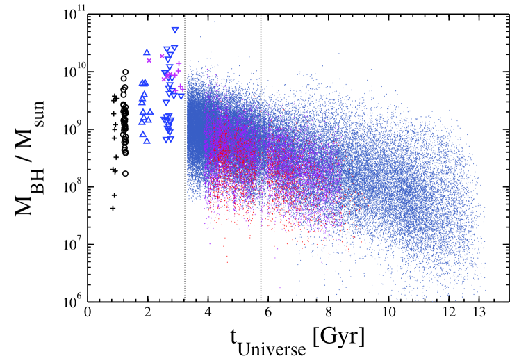
Figure 15: The evolution of $M_{\rm BH}$ along the age of the Universe for several of the samples studied here: the SDSS, 2QZ and 2SLAQ samples at $z<2$ (small blue, magenta and red points, respectively); the combined N07+S04 sample at $z\simeq 2.4$ and $\simeq 3.3$ (blue triangles); the $z>2$ sources from the M09 (magenta x-signs) and D09 (magenta crosses) samples; the T11 sources at $z\simeq 4.8$ (black circles); and a sample of $z\simeq 6.2$ sources, taken from the studies of Kurk et al. (2007) and Willott et al. (2010, black crosses). The $M_{\rm BH}$ estimates are based on H$\beta$ (for the N07+S04, D09, M09 and $z<0.75$ SDSS sources) or Mg ii (for the T11, $z\simeq 6.2$ and $z>0.75$ SDSS sources), following Eqs. 3 or 12, respectively. Dotted vertical lines mark $z=1$ and $2$.

Figure 16 shows the evolution of $L/L_{\rm Edd}$ with redshift for the SDSS sample studied here. We draw attention to the smooth transition seen in Fig. 16 at $z=0.75$. This region marks the transition from $M_{\rm BH}$ and $L/L_{\rm Edd}$ estimates that are based on H$\beta$ and $L_{5100}$, to those based on Mg ii and $L_{3000}$. As explained in §6.4, this transition wouldn’t appear as smooth if these quantities were obtained using the methods of McLure & Dunlop (2004) and Richards et al. (2006a). The steep rise of the upper envelope of the $L/L_{\rm Edd}$ distribution with redshift (see also NT07) flattens at $z\sim 1$, so that the highest-$L/L_{\rm Edd}$ sources approach the expected limit of $L/L_{\rm Edd}\simeq 1$. We stress that the upper envelope of the $L/L_{\rm Edd}$ distribution is not affected by selection effects related to the flux limits of the various samples. For example, an un-obscured AGN at $z=1.5$, powered by a SMBH with $M_{\rm BH}=10^{9}\,M_{\odot}$ and accreting at the Eddington limit could have easily been observed within the SDSS, since its observed $i$-band magnitude would be $\sim$16.4. Such a source would appear as a green point, at $z=1.5$ and $L/L_{\rm Edd}=1$ in Fig. 16 - a region in parameter space which is clearly dominated by sources with much lower $M_{\rm BH}$. Thus, Fig. 16 suggests that the vast majority of very massive BHs, with $M_{\rm BH}\raisebox{-2.15277pt}{$\;\stackrel{{\scriptstyle>}}{{\sim}}\;$}10^{9}\,M_{\odot}$, do not accrete close to their Eddington limit even at $z\sim 2$, which is often considered as “the epoch of peak Quasar activity”. Such SMBHs have probably experienced periods of faster mass accumulation at $z>3$ (Willott et al., 2010; De Rosa et al., 2011, T11). This scenario is supported by the extreme rareness of AGNs with $L_{\rm bol}>10^{47}$ at $z\sim 1-2$ (see, e.g., Croom et al., 2004; Hasinger et al., 2005; Richards et al., 2006b; Hopkins et al., 2007, and references therein). As mentioned above, the flux limits have a considerable influence on the faintest sources, and practically determine the low-end of theobserved distributions we present, at all accessible redshifts. Indeed, deeper surveys (e.g., zCOSMOS, VVDS) have revealed populations of $z\sim 1-2$ AGN with $L/L_{\rm Edd}\simeq 0.05$ (e.g. Gavignaud et al., 2008; Trump et al., 2009; Merloni et al., 2010).

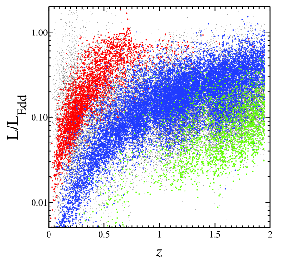
Figure 16: The evolution of $L/L_{\rm Edd}$ with redshift, for the entire SDSS sample studied here. Red, blue and green points highlight sub-samples of sources, with $M_{\rm BH}$ is in the range of $10^{7.5-7.8}$, $10^{8.5-8.8}$ and $10^{9.5-9.8}\,M_{\odot}$, respectively. Note the lack of very massive BHs that accrete at high rates (i.e. sources with $M_{\rm BH}>3\times 10^{9}\,M_{\odot}$ and $L/L_{\rm Edd}>0.2$) at $z<2$.

To conclude, in this first of two papers we presented a systematic study of the methods we use to measure $M_{\rm BH}$ and $L/L_{\rm Edd}$ in type-I AGN at $z\raisebox{-2.15277pt}{$\;\stackrel{{\scriptstyle>}}{{\sim}}\;$}1$. This was done through a combination of larger samples, spanning a broader range in redshift and luminosity, in comparison to previous works. We focused on the observables associated with the H$\beta$, Mg ii $\lambda 2798$ and C iv $\lambda 1549$ emission lines, as these are typically available for single epoch spectra of high-redshift sources. Our main findings are:

1. We provide a luminosity-dependent prescription for obtaining $L_{\rm bol}$ from $L_{3000}$. The resulting $L_{\rm bol}$ is consistent with the one obtained from $L_{5100}$ and differs by a factor of $\sim 1.5$ from previous estimates of this correction, for luminous sources.

2. The width of the Mg ii line was shown to follow closely the width of the H$\beta$ line up to ${\rm FWHM}\simeq 6000\,{\rm km\,s}^{-1}$, beyond which the Mg ii line width appears to saturate (§6.3).

3. We obtained an improved $\hbox{${R_{\rm BLR}}$}-L_{3000}$ relation, with a best-fit slope of 0.62, consistent with previous studies (e.g., McLure & Dunlop, 2004). We further find that the relation is probably luminosity-dependent and provide several alternative slopes and scalings. Combining this with point (ii) above, we obtained an $M_{\rm BH}$ estimator that is highly consistent with the H$\beta$-based one (Eq. 12). The scatter between the two is 0.32 dex (§6.4). This relation provides $M_{\rm BH}$ estimates that are systematically higher, by a factor of 1.75, than those of the McLure & Dunlop (2004) $M_{\rm BH}$ estimator.

4. The combination of points (i) and (iii) above produces Mg ii-based estimates of $L/L_{\rm Edd}$ that are systematically lower, by a factor of about 2.2, than those derived by previously published prescriptions.

5. The width of the C iv line shows no correlation with either H$\beta$ or Mg ii, and for most sources is substantially different from the what is expected from the virial assumption. The large scatter in the ratios of line widths ($\sim$0.5 dex) does not correlate with any other observable AGN property, and thus cannot be corrected for (§7). The problematic behavior of FWHM(C iv) dominates the associated virial products and practically prohibits any reliable measurements of $M_{\rm BH}$ using the C iv line.

6. We do not find a significant population of excessively massive BHs ($M_{\rm BH}>10^{9}\,M_{\odot}$) that accrete close to their Eddington limit. Such high mass BHs are observed as slowly accreting sources ($L/L_{\rm Edd}\sim 0.05-0.1$), as early as $z\simeq 2$ (Fig. 16), and might be observable in yet deeper surveys.

A full analysis of the evolutionary trends mentioned here, and others, will be presented in a forthcoming paper.

Two new relevant papers were published after the submission of the present paper to the journal. The study of Shen & Liu (2012) presented a new sample of 60 luminous SDSS AGN at $z\sim 1.5-2.2$, for which the C iv, Mg ii, H$\beta$ and H$\alpha$ lines were measured, using high quality NIR spectroscopy. The conclusions of the Shen & Liu (2012) study regarding the problematic usage of C iv as an $M_{\rm BH}$ estimator are in excellent agreement with our findings. In particular, Shen & Liu (2012) find a large discrepancy between FWHM(C iv) and FWHM(H$\beta$), and almost half of their sources show ${\rm FWHM}\left({\rm H}\beta\right)>{\rm FWHM}\left({\rm C}\,\textsc{iv}\right)$. The study of Ho et al. (2012) presented simultaneous rest-frame UV-to-optical spectra of 7 luminous AGN at $z\simeq 1.5$, which include the C iv, Mg ii, C iii] $\lambda 1909$ and H$\alpha$ lines. All Mg ii-based estimates of $M_{\rm BH}$ were shown to be consistent with those based on H$\alpha$, while C iv-based estimates of $M_{\rm BH}$ showed large discrepancies, of up to a factor of $\sim$5 (compared with $M_{\rm BH}$[H$\alpha$]). Thus, both the Shen & Liu (2012) and Ho et al. (2012) studies strengthen our conclusions, using additional high quality, high redshift samples.

9 Acknowledgments

We thank the anonymous referee for his/her careful reading of the manuscript and detailed comments, which allowed us to improve the paper. We thank Paola Marziani and Lutz Wisotzki for providing spectra and ancillary data for the HES sources; Gary Ferland for providing his Iron emission model; and Stephen Fine for providing 2SLAQ-related data and useful comments on the analysis of 2QZ and 2SLAQ sources. We also thank Yue Shen for useful comments. This study makes use of data from the SDSS (http://www.sdss.org/collaboration/credits.html). Funding for this work has been provided by the Israel Science Foundation grant 364/07 and by the Jack Adler Chair for Extragalactic Astronomy.

Appendix A Photometry-Based Flux Calibration for 2QZ and 2SLAQ Spectra

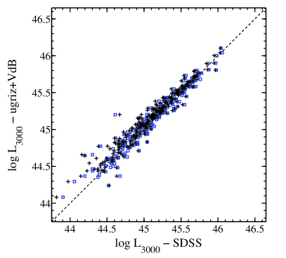
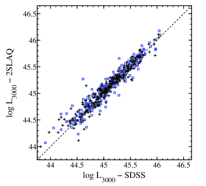
Figure 17: Comparison of $L_{3000}$, as measured from SDSS spectra and from our calibrated 2SLAQ spectra, for the 262 sources that have duplicate high-S/N spectroscopy of the Mg ii spectral region. Left: calibration obtained by the nearest photometric band and assuming the SED follows the uniform composite spectrum of Vanden Berk et al. (2001). Right: calibration obtained by fitting a power law to all the available SDSS ($ugriz$) magnitudes. In both panels, blue squares indicate luminosities measured directly from the observed spectra, while black crosses represent the results of our Mg ii-fitting procedure. The dashed lines represent the 1:1 relations.

Spectra obtained as part of the 2QZ and 2SLAQ surveys, using the AAT, are not flux calibrated. Previous studies used single-band magnitudes, in either the $b_{\rm J}$- or $g$ bands, to derive monochromatic luminosities, assuming all spectra follow a uniform UV-to-optical SED of $f_{\rm\nu}\propto\nu^{-0.5}$ (e.g., Croom et al., 2004; Richards et al., 2005; Fine et al., 2008). Here we employed a more robust flux calibration scheme, which relies on all the photometric data available in the 2QZ and 2SLAQ catalogs. All sources within the 2QZ catalog have tabulated $u$, $b_{\rm J}$ and $r$ band magnitudes, and all sources within the 2SLAQ catalog have the full set of $ugriz$ magnitudes. The following two procedures were tested using a unique sample of sources, which have duplicate spectroscopy from both the SDSS and 2SLAQ surveys, kindly provided by S. Fine. Although the original sample had 639 sources, here we focus only on the 262 sources that passed basic quality criteria, and that have $z<1.3$, in order to avoid the effects of the telluric features on the estimation of $L_{3000}$. The (fully calibrated) SDSS spectra of these sources were fitted using our Mg ii-fitting procedure (see §3).

First, we test how can the determination of monochromatic luminosities be improved if one uses the photometric band which is as close as possible to the (observed-frame) spectral region under question. In the case of $L_{3000}$, for sources at $z\simeq 1$, 1.5 or 2, the relevant bands are $r$, $i$ or $z$, respectively. To test this method for the 262 sources, we shifted the composite of VdB01 to the appropriate redshift and then scaled to the observed SDSS (AB) magnitude in the nearest available band. We used the full composite, including emission lines, and the scaling was done through synthetic photometry, using the entire passband of the relevant filter. Next, we measured the continuum flux density of the shifted and scaled template in a narrow band around (rest-frame) 3000Å, similarly to the main Mg ii fitting procedure. The left panel in Figure 17 compares $L_{3000}$ obtained through this method to the one measured from the SDSS spectra. The luminosity estimates are highly consistent with those derived from our Mg ii fits of the SDSS spectra - , the mean difference is 0.06 dex and the scatter around the 1:1 relation is 0.11 dex.

Since the method described above assumes a uniform SED, it necessarily results in calibrated spectra where ratios of $\lambda L_{\lambda}$ estimated at any two wavelength bands remain constant. In such a situation, there is no justification for re-calibrating any specific $\hbox{${R_{\rm BLR}}$}-\lambda L_{\lambda}$ relation, since all slopes will remain those of the initial relation ($\hbox{${R_{\rm BLR}}$}-L_{5100}$ in our case), and the change in scaling factors would only reflect the assumed (uniform) SED. Thus, we devised an additional method that attempts to overcome this issue.

We assume that each AAO-observed source can be described as a combination of a power-law continuum and an emission (and absorption) line spectrum. The power-law component is provided by a grid of spectra of the form $f_{\nu}\propto\nu^{\alpha}$, with $\alpha$ varying between -2 and 0 in steps of 0.05. Each uncalibrated spectrum is first smoothed using very broad boxcar averaging (251 pixels, i.e. $\sim$1080Å). Next, the input spectrum is divided by its smoothed version, to establish a (relative) emission line spectrum. The emission line spectrum is then multiplied by each of the power-law spectra in our grid. All such “combined” spectra are scaled to match the observed $r$ band magnitude of the source. Finally, the best combined spectrum is chosen, such that it best matches the observed $g$ or $b_{\rm J}$ magnitudes, for sources from the 2SLAQ or 2QZ catalogs, respectively. Figure 18 illustrates the resultant pseudo-calibrated spectrum of J003844.86-004404.5 ($z=0.6074$), observed as part of the 2SLAQ survey, compared with its SDSS spectrum. The right panel of Figure 17 compares $L_{3000}$ obtained through the power-law fitting method to the one measured from the SDSS spectra. The mean difference between the estimates if now merely 0.03 dex, and the scatter around the 1:1 relation is 0.10 dex, indistinguishable from the scatter found for the “uniform SED” method outlined above.

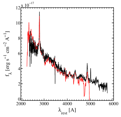
Figure 18: Example of a 2SLAQ spectrum, calibrated using our procedure, for object J003844.86-004404.5 ($z=0.6074$). The SDSS spectrum is shown in black (smoothed by a boxcar filter of 11 pixels). The 2SLAQ spectrum, calibrated using all the available SDSS photometry and a best-fit power law, is shown in red (smoothed over 9 pixels).

In conclusion, since the two methods provide consistent estimates of $L_{3000}$, both can be used in future studies that rely on 2QZ and 2SLAQ spectra of type-I AGN. However, only the full power-law fitting method allows for a non-uniform UV-optical continuum SED, and thus we adopt it in this paper.

Appendix B Additional Information on Small Samples

The following provides additional information on the literature samples used in this work.

• 59 PG quasars at $0.25\lesssim z\lesssim 0.5$, from the study of Baskin & Laor (2005, BL05 in the present paper). For these sources, the H$\beta$ line was observed as part of the survey of Boroson & Green (1992), and fitted using the procedure detailed in §3. From the original sample of 81 sources, we omit the 22 sources that were also studied in Shang et al. (2007, see below). The C iv line was observed as part of several HST and IUE campaigns, and the archival spectra were fitted by BL05. We adopt their C iv measurements (Table 1 of BL05) but use our own H$\beta$ fits.

• 44 sources at $z\simeq 2.4$ and $z\simeq 3.3$ from the study of (Netzer et al., 2007, N07 in the present paper), which incorporates also the sample presented in (Shemmer et al., 2004, S04 in the present paper). The C iv line was observed in a variety of optical surveys and the H$\beta$ line was observed in a dedicated H- and K-band campaign. All line measurements for this sample were carried out using the procedures detailed in §3.

• 22 PG quasars at $0.1\lesssim z\lesssim 0.4$ from the study of (Shang et al., 2007, Sh07 in the present paper). The C iv line was observed by the HST and the Mg ii and H$\beta$ lines were observed in a dedicated, almost-simultaneous ground-based optical campaign. This dataset is exceptionally useful for our analysis, due to the high quality of the observations & related calibrations, and the detailed measurements of H$\beta$, Mg ii and C iv for all 22 sources. We thus preferred the usage of these measurements over those reported in BL05 (see above), for all the Sh07 sources. We used the tabulated parameters of the Sh07 study for all lines, as well as the tabulated continuum parameters. However, since the Sh07 study fits a power law continuum over the entire (rest-frame) UV-optical range, the tabulated parameters underestimate $L_{3000}$ as defined here (see §3). We correct for this by applying the typical correction factor derived in §3.

• 90 sources at $z\lesssim 0.3$ from the study of (Sulentic et al., 2007, Sul07 in the present paper). This study presents a compilation of C iv measurements that are based on archival HST spectra of 130 sources, many of which overlap with the BL05 or Sh07 samples. We chose 90 sources for which H$\beta$ was reliably measured, by applying our fitting procedure to spectra obtained either from the SDSS or from the catalog of Marziani et al. (2003). We omitted all sources with $z<0.05$, to avoid severe host galaxy contamination. For the sake of consistency, we prefer our own fits over the H$\beta$ line measurements published within Marziani et al. (2003). For 11 sources, the SDSS spectra also cover the Mg ii line. These sources are thus part of the small subset of sources with measurements of all three emission lines. The SDSS counterparts are removed from the large SDSS sample.

• 19 SDSS sources at $z\simeq 0.36$ from the study of (McGill et al., 2008, Mc08 in the present paper) for which the Mg ii and H$\beta$ lines were observed in a dedicated Keck/LRIS campaign Woo et al. (2006). The SDSS spectra of these sources were removed from our SDSS sample.

• 10 sources at $z\sim 1-2.2$ from the study of (Dietrich et al., 2009, D09 in the present paper) for which the C iv (9 sources) and Mg ii (7 sources) lines were observed as part of several optical surveys. The H$\beta$ line was observed in a dedicated campaign in the $J$ and $H$ bands.

• 30 sources at $z\sim 1-2.4$ from the study of (Marziani et al., 2009, M09 in the present paper) for which the C iv line was observed as part of the Hamburg-ESO survey Wisotzki et al. (2000) and the H$\beta$ line was observed in the $sZ$, $J$ and $H$ bands.

• 40 sources at $z\simeq 4.8$ from the study of (Trakhtenbrot et al., 2011, T11 in the present paper) for which the C iv line was observed as part of the SDSS and the Mg ii lines were observed by a dedicated H- and K-band campaign. All line measurements for this sample were carried out using the procedures detailed in §3.

Appendix C Line Fitting

C.1 The H$\beta$ complex

We fitted the H$\beta$ line complex in a very similar manner to the one described in NT07. The linear continuum is fitted between two bands around either 4435Å or 4730Å and 5110Å. The continuum is subtracted from the observed spectrum and an initial fit of the narrow [O iii]$\lambda\lambda 4959,5007$Å lines is used in order to determine the systematic redshift and the velocity dispersion of the narrow line region (NLR) gas, so to assist with the full H$\beta$-[O iii] fit (see below). The two [O iii] lines are forced to have the same systematic shift and width, in the range $300<{\rm FWHM}<1200\,{\rm km\,s}^{-1}$, and a flux ratio of 1:3.

The grid of Fe ii templates is constructed by broadening and shifting the original template of Boroson & Green (1992). The convolution is preformed with a single Gaussian profile with a width that increases in steps of $25\,{\rm km\,s}^{-1}$, in the range of 1200 to 20000 km s^-1 . The templates are shifted in steps of 69 km s^-1 ($\sim$1Å), in the range of -1000 to +1000 km s^-1 . Our Fe ii grid thus consists of 23343 different, normalized, templates. The best-fit template is chosen through a standard $\chi^{2}$ minimization scheme, which focuses on the flux density in the 4400-4650Å range and provides the best-fitting scaling factor. The scaled best-fit template is then subtracted from the spectra so that the continuum can be re-measured. The process is repeated until we receive continuum- and iron-free spectra. Several of the samples considered here (N07; Sh07; M09; D09) were originally fitted by codes that neglected the possible shift of the Fe ii template. However, the differences in the main derived parameters ($L_{5100}$ and FWHM(H$\beta$)) are negligible (see Hu et al., 2008; Marziani & Sulentic, 2012).

Finally, we fit an emission line model which consists of 5 Gaussians: two broad and one narrow components for the H$\beta$ line and a single narrow component for each of the [O iii] lines. Each of the broad components is allowed to have a width in the range $1200<{\rm FWHM}<20000\,{\rm km\,s}^{-1}$, and to be shifted by as much as 1000 km s^-1 , relative to the redshift determined by the initial [O iii] fit. All three narrow components are forced to have the systemic shift and line widths. These are further constrained to differ only by as much as 200 km s^-1 (shift) and 30% (width), from the parameters determined in the initial [O iii] fit, but not to exceed the allowed range of $300<{\rm FWHM}<1200\,{\rm km\,s}^{-1}$. The flux ratio of the two [O iii] features is again fixed at 1:3, while the ratio between the narrow H$\beta$ component and the [O iii] $\lambda 5007$ line is free to take any value in the range of $0.05-1$ (i.e. the presence of any significant [O iii] signal dictates the presence of a narrow H$\beta$ component).

C.2 The Mg ii $\lambda 2798$ complex

We fit a linear pseudo-continuum is to the flux around 2655 and 3020Å. This component completely ignores the Balmer continuum emission and thus does not represent the “real” (accretion originated) underlying continuum emission. The typical difference between the “real” $F_{3000}$ and the one we measure here is, however, small. For example, combining the composite spectrum of VdB01 and the best-fit UV-optical power law continuum ($f_{\nu}\propto\nu^{-0.44}$) implies that the measured $F_{3000}$ is larger by a factor of 1.16. As a second test, we used the SDSS sample under study. The “real” 3000Å continuum was estimated by fitting a power law between narrow bands at 2200 and 4200Å. This limits the test to sources with $0.75<z<1.2$. The observed $F_{3000}$ was measured by applying the full-scale Mg ii-fitting procedure. The resulting median factor for these 14532 sources is 1.15 with a standard deviation of 0.06 dex ($10\%$). We use this factor to convert the “real” $L_{3000}$ measurements of the Sh07 samples, to match our $L_{3000}$ measurements.

We use a Fe ii & Fe iii template made of the composite prepared by Vestergaard & Wilkes (2001) and several additional Fe ii lines in the region not covered by the above composite, kindly provided by G. Ferland (private communication). The new lines are similar to the ones presented in Sigut & Pradhan (2003, Fig. 13) and in Baldwin et al. (2004, Fig. 5). The Fe ii flux under the Mg ii line is dominated by the red extension of the $\sim$2750Å emission complex. The additional flux tends to flatten in sources with very broad Fe ii lines, but the overall effect on the Mg ii fitting is very small. We consider this template to be more reliable than the addition of constant flux under the Mg ii line, as done by, e.g., Kurk et al. (2007) and Fine et al. (2008). Other studies, such as Salviander et al. (2007) and Shen et al. (2008), use templates that are very similar to ours, following the models in Sigut & Pradhan (2003). A visual inspection of the spectra suggests that the iron lines blueward and redward of Mg ii must not share a common scale factor. Instead, our procedure finds the template which best fits the spectrum in the range of 2600-2700Å, in terms of shift and width of the Iron features. The scaling in the 2900-3030Å region is allowed to vary by up to 15%. We then combine the two templates, characterized by the same shift and width, so that they join at 2810Å.

Each of the two doublet profiles consists of two broad and one narrow emission Gaussians, and a single (narrow) absorption Gaussian. We have fixed the intensity ratio of the two broad Mg ii doublet components to 1:1, suitable for optically-thick lines, while for the narrow components the ration is 1:2. Since the narrow emission component of Mg ii is difficult to disentangle, we have experimented with an alternative procedure in which the width of the narrow Mg ii line was bound to match the one measured from the [O iii] $\lambda 5007$ line, in sources where both are observed (the SDSS “H$\beta$$\times$Mg ii” sub-sample). This technique resulted in either a width which is similar to the one achieved by the free-fitting version, or in a fit of inferior quality. Our preferred procedure is, therefore, to freely fit the narrow Mg ii doublet components with the additional constraints of $300<{\rm FWHM}<1200\,{\rm km\,s}^{-1}$, and a shift of no more than 200 km s^-1 , relative to the systemic redshift. The broad components are allowed to have $1200<{\rm FWHM}<15000\,{\rm km\,s}^{-1}$, and to be shifted by as much as 1000 km s^-1 . The (narrow) absorption feature is set to have a doublet Gaussian profile with and is allowed to have $150<{\rm FWHM}<2000\,{\rm km\,s}^{-1}$, and a center which is blue-shifted by as much as 5000 km s^-1 , with respect to the expected (laboratory) wavelengths of the Mg ii doublet, assuming the systemic redshift. As with the other line-fitting parameters, we verified that these choices capture the properties of the vast majority of sources that show such absorption features, while not affecting the quality of the broad Mg ii profile fit.

C.3 The C iv $\lambda 1549$ complex

Our procedure closely follows the one presented in Fine et al. (2010) and we refer the reader to the very thorough discussion in their Appendix A. In particular, we do not fit the weak Fe ii features around the C iv line.

The components of our C iv line model are very similar to those of the Mg ii line model (see  C.2 above). Each of the two doublet profiles consists of two broad and one narrow emission Gaussians, and a single (narrow) absorption Gaussian, with the intensity ratios following the same scaling as for Mg ii. The broad components are allowed to have line widths in the range $1200<{\rm FWHM}<15000\,{\rm km\,s}^{-1}$, and to have shifts in the range of -3000 to +1500 km s^-1 , thus taking into account significantly blueshited C iv profiles, which are often observed in type-I AGN (Richards et al., 2011, and references therein). The narrow components are allowed to have $300<{\rm FWHM}<1200\,{\rm km\,s}^{-1}$, and to be shifted by as much as 200 km s^-1 . We note that our choice to include a narrow emission component does not mean that such a component contributed significantly to the line profile. Indeed, several studies claimed that the narrow emission component in C iv is very weak, or non-existent altogether (see, e.g., Wills et al. 1993, BL05 and the discussion in Vestergaard & Peterson, 2006). Although our code allowed the peak intensity of the narrow component to reach 0.5 that of the broad components, its actual contribution to the overall fitted C iv line profile is indeed found to be insignificant. For the SDSS “Mg ii$\times$C iv”sub-sample, the median of the EW(C iv,NLR)/EW(C iv,BLR) ratio is only$\sim 0.007$, while for 99% of the sources this ratio is smaller than about 0.05 and for 25% of the sources it is completely negligible (i.e., $<0.001$). Thus, the inclusion of a narrow C iv component is not expected to significantly affect measurements of the broad component of the line, which we use throughout the present work. This also justifies our usage of broad-C iv measurements that include (e.g., BL05) or don’t include (e.g., Sh07) a narrow C iv component. The narrow absorption feature is set in the same manner as in the case of the Mg ii line (see C.2 above).

We also assigned a single broad Gaussian component to each of the He ii $\lambda 1640$, O iii] $\lambda 1663$ and N iv] $\lambda 1486$ lines, which are forced to have a common line width, in the rage of $1200<{\rm FWHM}<8200\,{\rm km\,s}^{-1}$, and a common shift, in the range of -1500 to +750 km s^-1 . As mentioned in Fine et al. (2010), these features may in practice account for emission which originates either from Fe ii or other, unresolved, lines (e.g., Al ii $\lambda 1671$). The derived properties of these lines are not used to infer the physical parameters of the BLR gas.

References

- Abazajian et al. (2009) Abazajian, K. N., et al. 2009, The Astrophysical Journal Supplement Series, 182, 543
- Akritas & Bershady (1996) Akritas, M. G., & Bershady, M. A. 1996, The Astrophysical Journal, 470, 706
- Assef et al. (2011) Assef, R. J., et al. 2011, The Astrophysical Journal, 742, 93
- Baldwin (1977) Baldwin, J. A. 1977, The Astrophysical Journal, 214, 679
- Baldwin et al. (2004) Baldwin, J. A., Ferland, G. J., Korista, K. T., Hamann, F., & LaCluyze, A. 2004, The Astrophysical Journal, 615, 610
- Baskin & Laor (2005) Baskin, A., & Laor, A. 2005, Monthly Notices of the Royal Astronomical Society, 356, 1029 (BL05)
- Becker et al. (1995) Becker, R. H., White, R. L., & Helfand, D. J. 1995, The Astrophysical Journal, 450, 559
- Bentz et al. (2009) Bentz, M. C., Peterson, B. M., Netzer, H., Pogge, R. W., & Vestergaard, M. 2009, The Astrophysical Journal, 697, 160
- Bianchi et al. (2009) Bianchi, S., Guainazzi, M., Matt, G., Fonseca Bonilla, N., & Ponti, G. 2009, Astronomy and Astrophysics, 495, 421
- Boroson & Green (1992) Boroson, T. A., & Green, R. F. 1992, The Astrophysical Journal Supplement Series, 80, 109
- Cardelli et al. (1989) Cardelli, J. A., Clayton, G. C., & Mathis, J. S. 1989, The Astrophysical Journal, 345, 245
- Clavel et al. (1991) Clavel, J., et al. 1991, The Astrophysical Journal, 366, 64
- Corbin & Boroson (1996) Corbin, M. R., & Boroson, T. A. 1996, The Astrophysical Journal Supplement Series, 107, 69
- Croom et al. (2004) Croom, S. M., Smith, R. J., Boyle, B. J., Shanks, T., Miller, L., Outram, P. J., & Loaring, N. 2004, Monthly Notices of the Royal Astronomical Society, 349, 1397
- Croom et al. (2008) Croom, S. M., et al. 2008, Monthly Notices of the Royal Astronomical Society, 392, 19
- Croom (2011) Croom, S. M. 2011, The Astrophysical Journal, 736, 161
- De Rosa et al. (2011) De Rosa, G., Decarli, R., Walter, F., Fan, X., Jiang, L., Kurk, J. D., Pasquali, A., & Rix, H. W. 2011, The Astrophysical Journal, 739, 56
- Dietrich et al. (2009) Dietrich, M., Mathur, S., Grupe, D., & Komossa, S. 2009, The Astrophysical Journal, 696, 1998 (D09)
- Elvis et al. (1994) Elvis, M., et al. 1994, The Astrophysical Journal Supplement Series, 95, 1
- Fine et al. (2010) Fine, S., Croom, S. M., Bland-Hawthorn, J., Pimbblet, K. A., Ross, N. P., Schneider, D. P., & Shanks, T. 2010, Monthly Notices of the Royal Astronomical Society, 409, 591
- Fine et al. (2006) Fine, S., et al. 2006, Monthly Notices of the Royal Astronomical Society, 373, 613
- Fine et al. (2008) —. 2008, Monthly Notices of the Royal Astronomical Society, 390, 1413
- Gavignaud et al. (2008) Gavignaud, I., et al. 2008, Astronomy and Astrophysics, 492, 637
- Gibson et al. (2009) Gibson, R. R., et al. 2009, The Astrophysical Journal, 692, 758
- Graham et al. (2011) Graham, A. W., Onken, C. a., Athanassoula, E., & Combes, F. 2011, Monthly Notices of the Royal Astronomical Society, 412, 2211
- Greene & Ho (2005) Greene, J. E., & Ho, L. C. 2005, The Astrophysical Journal, 630, 122
- Hasinger et al. (2005) Hasinger, G., Miyaji, T., & Schmidt, M. 2005, Astronomy and Astrophysics, 441, 417
- Ho et al. (2012) Ho, L. C., Goldoni, P., Dong, X.-B., Greene, J. E., & Ponti, G. 2012, The Astrophysical Journal, 754, 11
- Hopkins et al. (2007) Hopkins, P. F., Richards, G. T., & Hernquist, L. 2007, The Astrophysical Journal, 654, 731
- Hu et al. (2008) Hu, C., Wang, J., Ho, L. C., Chen, Y., Zhang, H.-T., Bian, W., & Xue, S.-J. 2008, The Astrophysical Journal, 687, 78
- Jin et al. (2012) Jin, C., Ward, M., Done, C., & Gelbord, J. 2012, Monthly Notices of the Royal Astronomical Society, 420, 1825
- Kaspi et al. (2007) Kaspi, S., Brandt, W. N., Maoz, D., Netzer, H., Schneider, D. P., & Shemmer, O. 2007, The Astrophysical Journal, 659, 997
- Kaspi et al. (2005) Kaspi, S., Maoz, D., Netzer, H., Peterson, B. M., Vestergaard, M., & Jannuzi, B. T. 2005, The Astrophysical Journal, 629, 61
- Kaspi et al. (2000) Kaspi, S., Smith, P. S., Netzer, H., Maoz, D., Jannuzi, B. T., & Giveon, U. 2000, The Astrophysical Journal, 533, 631
- Kellermann et al. (1989) Kellermann, K. I., Sramek, R., Schmidt, M., Shaffer, D. B., & Green, R. F. 1989, The Astronomical Journal, 98, 1195
- Kelly et al. (2010) Kelly, B. C., Vestergaard, M., Fan, X., Hopkins, P. F., Hernquist, L., & Siemiginowska, A. 2010, The Astrophysical Journal, 719, 1315
- Kurk et al. (2007) Kurk, J. D., et al. 2007, The Astrophysical Journal, 669, 32
- Marconi et al. (2004) Marconi, A., Risaliti, G., Gilli, R., Hunt, L. K., Maiolino, R., & Salvati, M. 2004, Monthly Notices of the Royal Astronomical Society, 351, 169
- Marziani & Sulentic (2012) Marziani, P., & Sulentic, J. W. 2012, New Astronomy Reviews, 56, 49
- Marziani et al. (2009) Marziani, P., Sulentic, J. W., Stirpe, G. M., Zamfir, S., & Calvani, M. 2009, Astronomy and Astrophysics, 495, 83 (M09)
- Marziani et al. (2003) Marziani, P., Sulentic, J. W., Zamanov, R., Calvani, M., Dultzin, D., Bachev, R., & Zwitter, T. 2003, The Astrophysical Journal Supplement Series, 145, 199
- McConnell et al. (2011) McConnell, N. J., Ma, C.-p., Gebhardt, K., Wright, S. A., Murphy, J. D., Lauer, T. R., Graham, J. R., & Richstone, D. O. 2011, Nature, 480, 215
- McGill et al. (2008) McGill, K. L., Woo, J., Treu, T., & Malkan, M. A. 2008, The Astrophysical Journal, 673, 703 (Mc08)
- McLure & Dunlop (2004) McLure, R. J., & Dunlop, J. S. 2004, Monthly Notices of the Royal Astronomical Society, 352, 1390 (MD04)
- McLure & Jarvis (2002) McLure, R. J., & Jarvis, M. J. 2002, Monthly Notices of the Royal Astronomical Society, 337, 109
- Merloni et al. (2010) Merloni, A., et al. 2010, The Astrophysical Journal, 708, 137
- Metzroth et al. (2006) Metzroth, K. G., Onken, C. A., & Peterson, B. M. 2006, The Astrophysical Journal, 647, 901
- Netzer et al. (2007) Netzer, H., Lira, P., Trakhtenbrot, B., Shemmer, O., & Cury, I. 2007, The Astrophysical Journal, 671, 1256 (N07)
- Netzer & Marziani (2010) Netzer, H., & Marziani, P. 2010, The Astrophysical Journal, 724, 318
- Netzer & Trakhtenbrot (2007) Netzer, H., & Trakhtenbrot, B. 2007, The Astrophysical Journal, 654, 754 (NT07)
- Onken et al. (2004) Onken, C. a., Ferrarese, L., Merritt, D., Peterson, B. M., Pogge, R. W., Vestergaard, M., & Wandel, A. 2004, The Astrophysical Journal, 615, 645
- Onken & Kollmeier (2008) Onken, C. A., & Kollmeier, J. A. 2008, The Astrophysical Journal, 689, L13
- Peterson et al. (2004) Peterson, B. M., et al. 2004, The Astrophysical Journal, 613, 682
- Press (2002) Press, W. H. 2002, Numerical recipes in C++ : the art of scientific computing
- Rafiee & Hall (2011) Rafiee, A., & Hall, P. B. 2011, The Astrophysical Journal Supplement Series, 194, 42
- Richards et al. (2005) Richards, G. T., et al. 2005, Monthly Notices of the Royal Astronomical Society, 360, 839
- Richards et al. (2006a) —. 2006a, The Astrophysical Journal Supplement Series, 166, 470
- Richards et al. (2006b) —. 2006b, The Astronomical Journal, 131, 2766
- Richards et al. (2011) —. 2011, The Astronomical Journal, 141, 167
- Runnoe et al. (2012) Runnoe, J. C., Brotherton, M. S., & Shang, Z. 2012, Monthly Notices of the Royal Astronomical Society, 422, 478
- Salviander et al. (2007) Salviander, S., Shields, Gregory A., Gebhardt, K., & Bonning, E. W. 2007, The Astrophysical Journal, 662, 131
- Schlegel et al. (1998) Schlegel, D. J., Finkbeiner, D. P., & Davis, M. 1998, The Astrophysical Journal, 500, 525
- Schneider et al. (2010) Schneider, D. P., et al. 2010, The Astronomical Journal, 139, 2360
- Shang et al. (2007) Shang, Z., Wills, B. J., Wills, D., & Brotherton, M. S. 2007, The Astronomical Journal, 134, 294 (Sh07)
- Shemmer et al. (2004) Shemmer, O., Netzer, H., Maiolino, R., Oliva, E., Croom, S. M., Corbett, E., & di Fabrizio, L. 2004, The Astrophysical Journal, 614, 547 (S04)
- Shen et al. (2008) Shen, Y., Greene, J. E., Strauss, M. A., Richards, G. T., & Schneider, D. P. 2008, The Astrophysical Journal, 680, 169
- Shen & Liu (2012) Shen, Y., & Liu, X. 2012, The Astrophysical Journal, 753, 125
- Shen et al. (2011) Shen, Y., et al. 2011, The Astrophysical Journal Supplement Series, 194, 45
- Sigut & Pradhan (2003) Sigut, T. a. a., & Pradhan, A. K. 2003, The Astrophysical Journal Supplement Series, 145, 15
- Stern & Laor (2012) Stern, J., & Laor, A. 2012, Monthly Notices of the Royal Astronomical Society, 423, 600
- Sulentic et al. (2007) Sulentic, J. W., Bachev, R., Marziani, P., Negrete, C. A., & Dultzin, D. 2007, The Astrophysical Journal, 666, 757 (Sul07)