First-order convex feasibility algorithms for X-ray CT

Abstract

PURPOSE: Iterative image reconstruction (IIR) algorithms in Computed Tomography (CT) are based on algorithms for solving a particular optimization problem. Design of the IIR algorithm, therefore, is aided by knowledge of the solution to the optimization problem on which it is based. Often times, however, it is impractical to achieve accurate solution to the optimization problem of interest, which complicates design of IIR algorithms. This issue is particularly acute for CT with a limited angular-range scan, which leads to poorly conditioned system matrices and difficult to solve optimization problems. In this article, we develop IIR algorithms which solve a certain type of optimization called convex feasibility. The convex feasibility approach can provide alternatives to unconstrained optimization approaches and at the same time allow for rapidly convergent algorithms for their solution – thereby facilitating the IIR algorithm design process.

METHOD: An accelerated version of the Chambolle-Pock (CP) algorithm is adapted to various convex feasibility problems of potential interest to IIR in CT. One of the proposed problems is seen to be equivalent to least-squares minimization, and two other problems provide alternatives to penalized, least-squares minimization.

RESULTS: The accelerated CP algorithms are demonstrated on a simulation of circular fan-beam CT with a limited scanning arc of 144^∘. The CP algorithms are seen in the empirical results to converge to the solution of their respective convex feasibility problems.

CONCLUSION: Formulation of convex feasibility problems can provide a useful alternative to unconstrained optimization when designing IIR algorithms for CT. The approach is amenable to recent methods for accelerating first-order algorithms which may be particularly useful for CT with limited angular-range scanning. The present article demonstrates the methodology, and future work will illustrate its utility in actual CT application.

I Introduction

Iterative image reconstruction (IIR) algorithms in computed tomography (CT) are designed based on some form of optimization. When designing IIR algorithms to account for various factors in the CT model, the actual designing occurs usually at the optimization problem and not the individual processing steps of the IIR algorithm. Once the optimization problem is established, algorithms are developed to solve it. Achieving convergent algorithms is important, because they yield access to the designed solution of the optimization problem and allow for direct assessment of what factors to include in a particular optimization problem. Convergent algorithms can also aid in determining at what iteration number to truncate an IIR algorithm. With access to the designed solution, the difference between it and previous iterates can be quantitatively evaluated to see whether this difference is significant with respect to a given CT imaging task.

It can be challenging to develop convergent algorithms for some optimization problems of interest. This issue is particularly acute for CT, which involves large-scale optimization. In using the term “large-scale”, we are specifically referring to optimization problems based on a linear data model, and the dimension of the linear system is so large that the system matrix cannot be explicitly computed and stored in memory. Such systems only allow for algorithms which employ operations of a similar computational expense to matrix-vector products. Large-scale optimization algorithms are generally restricted to first-order methods, where only gradient information on the objective function is used, or row-action algorithms such as the algebraic reconstruction technique (ART) Gordon:70 ; Herman . Recently, there has been renewed interest in developing convergent algorithms for optimization problems involving $\ell_{1}$-based image norms, and only in the last couple of years have practical, convergent algorithms been developed to solve these optimization problems for IIR in CT Jensen2011 ; Defrise:11 ; fessler:2012 ; SidkyCP:2012 . Despite the progress in algorithms, there are still CT configurations of practical interest, which can lead to optimization problems that can be quite challenging to solve accurately. Of particular interest in this work is CT with a limited angular-range scanning arc. Such a configuration is relevant to many C-arm CT and tomosynthesis applications. Modeling limited angular-range scanning, leads to system matrices with unfavorable singular value spectra and optimization problems for which many algorithms converge slowly.

In this article, we consider application of convex feasibility combettes1996convex ; combettes1993foundations to IIR for CT. In convex feasibility, various constraints on properties of the image are formulated so that each of these constraints specifies a convex set. Taking the intersection of all of the convex sets yields a single convex set, and the idea is to simply choose one of these images in the intersection set. We have found convex feasibility to be useful for CT IIR algorithm design Han:2012 , and it is of particular interest here for limited angular-range CT, because convex feasibility is amenable to recent accelerated first-order algorithms proposed by Chambolle and Pock (CP) chambolle2011first . In Sec. II, we specify the limited angular-range CT system, discuss unconstrained optimization approaches, and then list three useful convex feasibility problems along with a corresponding accelerated CP algorithm. In Sec. III, the accelerated convex feasibility CP algorithms are demonstrated with simulated CT projection data.

II Methods: Chambolle-Pock algorithms for convex feasibility

For this article, we focus on modeling circular, fan-beam CT with a limited scanning angular range. As with most work on IIR, the data model is discrete-to-discrete (DD) and can be written as a linear equation

$$\mathbf{g}=\mathit{X}\mathbf{f},$$ (1)

where $\mathbf{f}$ is the image vector comprised of pixel coefficients, $\mathit{X}$ is the system matrix generated by computing the ray-integrals with the line-intersection method, and $\mathbf{g}$ is the data vector containing the estimated projection samples. For the present investigation on IIR algorithms, we consider a single configuration for limited angular range scanning where the system matrix $\mathit{X}$ has a left-inverse ($\mathit{X}^{T}\mathit{X}$ is invertible) but is numerically unstable in the sense that it has a large condition number. The vector $\mathbf{f}$ consists of the pixels within a circle inscribed in a 256$\times$256 pixel array; the total number of pixels is 51,468. The sinogram contains 128 views spanning a 144^∘ scanning arc, and the projections are taken on a 512-bin linear detector array. The modeled source-to-isocenter and source-to-detector distances are 40 and 80 cm, respectively. The total number of transmission measurements is 65,536, and as a result the system matrix $\mathit{X}$ has about 25% more rows than columns. The condition of $\mathit{X}$, however, is poor, which can be understood by considering the corresponding continuous-to-continuous (CC) fan-beam transform. A sufficient angular range for stable inversion of the CC fan-beam transform requires a 208^∘ scanning arc (180^∘ plus the fan-angle, see for example Sec. 3.5 of Ref. Kak ). By using the inverse power method, as described in Ref. jakob:2011 , the condition number, the ratio of the largest to smallest singular value, for $\mathit{X}$ is determined to be $2.55\times 10^{4}$. One effect of the large condition number is to amplify noise present in the data, but it also can cause slow convergence for optimization-based IIR.

II.1 Unconstrained optimization for IIR in CT

Image reconstruction using this DD data model is usually performed with some form of optimization, because physical factors and inaccuracy of the model render Eq. (1) inconsistent – namely, no $\mathbf{f}$ exists satisfying this equation. Typically in using this model, quadratic optimization problems are formulated, the simplest of which is the least-squares problem

$$\mathbf{f}^{\circ}=\operatorname*{arg\,min}_{\mathbf{f}}\left\{\frac{1}{2}\|\mathbf{g}-\mathit{X}\mathbf{f}\|^{2}_{2}\right\},$$ (2)

where $\mathbf{f}^{\circ}$ is the image which minimizes the Euclidean distance between the available data $\mathbf{g}$ and the estimated data $\mathit{X}\mathbf{f}$. In the remainder of the article, we use the superscript “^∘” to indicate a solution to an optimization problem. Taking the gradient of this objective function, and setting it to zero component-wise, leads to the following consistent linear equation

$$\mathit{X}^{T}\mathit{X}\mathbf{f}=\mathit{X}^{T}\mathbf{g},$$ (3)

where the superscript $T$ denotes the matrix transpose. This linear equation is particularly useful for setting up the linear conjugate gradients (CG) algorithm, see for example Ref. Nocedal:06 , which has been used as the gold standard algorithm for large-scale quadratic optimization problems in IIR. The reader is also referred to conjugate gradients least-squares (CGLS) and LSQR (an algorithm for sparse linear equations and sparse least squares), which solve Eq. (2) for non-symmetric $\mathit{X}$ Paige:1982 .

The solution to Eq. (2) or (3) can be undesirable because of inconsistency in the data. Particularly for the present case, the poor conditioning of $\mathit{X}$ can yield tremendously amplified artifacts in the reconstructed image. As is well-known, artifacts due to data inconsistency can be controlled in optimization-based IIR by adding a penalty term to discourage large variations between neighboring pixels

$$\mathbf{f}^{\circ}=\operatorname*{arg\,min}_{\mathbf{f}}\left\{\frac{1}{2}\|\mathbf{g}-\mathit{X}\mathbf{f}\|^{2}_{2}+\alpha R(\mathbf{f})\right\},$$ (4)

where $R(\mathbf{f})$ is a generic roughness term which usually is a convex function of the difference between neighboring pixels in the image. The parameter $\alpha$ controls the strength of the penalty with larger values leading to smoother images. When $R(\mathbf{f})$ is chosen to be quadratic in the pixel values, the optimization problem can be solved by a host of standard algorithms including CG. Of recent interest have been convex regularizers based on the $\ell_{1}$-norm, which is more difficult to treat and, accordingly, for which many new, convergent algorithms have been proposed and applied to image reconstruction in CT Jensen2011 ; Defrise:11 ; fessler:2012 ; SidkyCP:2012 .

II.2 Convex feasibility

In this article, we consider convex feasibility problems which provide alternatives to the above-mentioned optimization problems. For convex feasibility problems, convex sets resulting from constraints on various properties of the image are formulated, and a single image which satisfies all the imposed constraints is sought. Most algorithms for such problems are based on projection onto convex sets (POCS) combettes1993foundations , where the image estimate is sequentially projected onto each constraint set. Convex feasibility problems can be: inconsistent, no image satisfies all the constraints; or consistent, at least one image satisfies all the constraints. In either case, POCS algorithms can yield a useful solution. In the inconsistent case, POCS algorithms can be designed to yield an image “close” to satisfying all the constraints. In the consistent case, a POCS algorithm can be designed to find an image obeying all the constraints. In either case, the issue of uniqueness is secondary, as an image “in the middle” of many inconsistent constraints or in the intersection set of consistent constraints is considered to be equally valid. Accordingly, the POCS result often depends on starting image, relaxation schemes, and projection order.

For our purposes we write a general convex feasibility as the following optimization problem

$$\mathbf{f}^{\circ}=\operatorname*{arg\,min}_{\mathbf{f}}\left\{\sum_{i}\delta_{S_{i}}(\mathit{K}_{i}(\mathbf{f}))\right\},$$ (5)

$\mathit{K}_{i}(\cdot)$ is the $i$th affine transform of the image $\mathbf{f}$; $S_{i}$ is the $i$th convex set to which $\mathit{K}_{i}(\mathbf{f})$ belongs; and the indicator function $\delta$ is defined

$$\delta_{S}(\mathbf{x})=\begin{cases}0&\mathbf{x}\in S\\ \infty&\mathbf{x}\not\in S\end{cases}.$$ (6)

The use of indicator functions in convex analysis provides a means to turn convex sets into convex functions rockafellar1970convex , and in this case, they allow convex feasibility problems to be written as a minimization of a single objective function. The objective function in Eq. (5) is zero for any image $\mathbf{f}$ satisfying all the constraints, i.e. $\mathit{K}_{i}(\mathbf{f})\in S_{i}$ for all $i$, and it is infinity if any of the constraints are violated. For a consistent convex feasibility problem, the objective minimum is zero, and for an inconsistent convex feasibility problem, the objective minimum is infinity.

II.3 Modified convex feasibility optimization and the Chambolle-Pock primal-dual algorithm

To solve the generic convex feasibility problem in Eq. (5), we modify this optimization problem by adding a quadratic term

$$\mathbf{f}^{\circ}=\operatorname*{arg\,min}_{\mathbf{f}}\left\{\frac{1}{2}\|\mathbf{f}-\mathbf{f}_{\text{prior}}\|^{2}_{2}+\sum_{i}\delta_{S_{i}}(\mathit{K}_{i}(\mathbf{f}))\right\},$$ (7)

where $\mathbf{f}_{\text{prior}}$ is a prior image estimate that can be set to zero if no prior image is available. With this optimization problem, we actually specify a unique solution to our generic convex feasibility problem in the consistent case – namely the image satisfying all constraints and closest to $\mathbf{f}_{\text{prior}}$. As we will demonstrate the algorithm we propose to use for solving Eq. (7) appears to yield useful solutions for the inconsistent case. This latter property can be important for IIR in CT because the data model in Eq. (1) is often inconsistent with the available projection data.

The reason for recasting the optimization problem in the form shown in Eq. (7) is that this optimization problem can be solved by an accelerated algorithm described in Ref. chambolle2011first . Recently, we have been interested in a convex optimization framework and algorithms derived by Chambolle and Pock (CP) chambolle2011first ; Pock2011 . This framework centers on the generic convex optimization problem

$$p^{\circ}=\min_{\mathbf{x}}\;\left\{G(\mathbf{x})+F(\mathit{H}\mathbf{x})\right\},$$ (8)

where $G(\cdot)$ and $F(\cdot)$ are convex functions, and $\mathit{H}$ is a linear transform. The objective function

$$p=G(\mathbf{x})+F(\mathit{H}\mathbf{x})$$

is referred to as the primal objective. This generic problem encompasses many optimization problems of interest to IIR in CT, because non-smooth convex functions such as the indicator and $\ell_{1}$-norm can be incorporated into $F$ or $G$. Also, the linear transform $\mathit{H}$ can model projection, for a data fidelity term, or a finite-difference-based gradient, for an image total variation (TV) term. The CP framework, as presented in Ref. chambolle2011first , comes with four algorithms that have different worst-case convergence rates depending on convexity properties of $F$ and $G$. Let $N$ be the number of iterations, the algorithm summaries are:

CP Algorithm 1

This basic CP algorithm forms the basis of the subsequent algorithms and it only requires $F$ and $G$ to be convex. The worst-case convergence rate is $O(1/N)$.

CP Algorithm 2

Can be used if either $F$ or $G$ are uniformly convex. Modifies CP Algorithm 1 using a step-size formula developed by Nesterov nesterov1983method ; beck:09 . The worst-case convergence rate is $O(1/N^{2})$. Because the convergence rate is faster than the previous case, this algorithm is an accelerated version of CP Algorithm 1.

CP Algorithm 3

Can be used if both $F$ and $G$ are uniformly convex. This algorithm is the same as CP Algorithm 1, except that there is a specific choice of algorithm parameters, depending on constants related to the uniform convexity of $F$ and $G$. The worst-case convergence is linear, i.e. $O(1/c^{N})$, where $c>1$ is a constant.

CP Algorithm 4

A simpler version of CP Algorithm 2, which also requires $F$ or $G$ to be uniformly convex. The convergence rate is slightly worse than $O(1/N^{2})$.

In a previous publication SidkyCP:2012 , we illustrated how to use CP Algorithm 1 from Ref. chambolle2011first to prototype many optimization problems of potential interest to image reconstruction in CT. We were restricted to CP Algorithm 1, because we considered mainly problem where $G$ was 0, and $F$ contained indicator functions, the $\ell_{1}$-norm, or TV terms and accordingly $F$ was not uniformly convex. In the present work, we narrow the class of optimization problems to those which can be written in the form of Eq. (7), where the sets $S_{i}$ are simple enough that direct Euclidean projections to the sets $S_{i}$ are analytically available. In matching up Eq. (7) to the generic optimization problem in Eq. (8) the function $G$ is assigned the uniformly convex quadratic term and $F$ gets the sum of indicator functions. As such, Eq. (7) fills the requirements of CP Algorithms 2 and 4. In the particular case of Eq. (7) the uniformly convex term, $0.5\|\mathbf{f}-\mathbf{f}_{\text{prior}}\|^{2}_{2}$, is simple enough that CP Algorithm 2 can be derived without any difficulty. Because this algorithm is an accelerated version of CP Algorithm 1, we refer to it, here, as the accelerated CP algorithm. This algorithm acceleration is particularly important for IIR involving an ill-conditioned data model such as Eq. (1) in the case of limited angular range scanning.

II.4 The primal-dual gap and convergence criteria

The CP algorithms are primal-dual in that they solve the primal minimization problem Eq. (8) together with a dual maximization problem

$$d^{\circ}=\max_{\mathbf{y}}\;\left\{-F^{*}(\mathbf{y})-G^{*}(-\mathit{H}^{T}\mathbf{y})\right\},$$ (9)

and,

$$d=-F^{*}(\mathbf{y})-G^{*}(-\mathit{H}^{T}\mathbf{y})$$

is the dual objective function, and the superscript ^∗ represents convex conjugation through the Legendre transform

$$P^{*}(\mathbf{z})=\max_{\mathbf{z}^{\prime}}\;\left\{\mathbf{z}^{T}\mathbf{z}^{\prime}-P(\mathbf{z}^{\prime})\right\}.$$ (10)

That the CP algorithms obtain the dual solution, also, is useful for obtaining a robust convergence criterion that applies for non-smooth convex optimization. As long as the primal objective function $p$ is convex, we have $p^{\circ}=d^{\circ}$. While a solution for a smooth optimization problem can be checked by observing that the gradient of the primal objective function in Eq. (8) is zero, this test may not be applicable to non-smooth optimization problems, where the primal objective function may not be differentiable at its minimum. Instead, we can use the primal-dual gap $p-d$, because the primal objective function for any $\mathbf{x}$ is larger than the dual objective function in Eq. (9) for any $\mathbf{y}$ except when $\mathbf{x}$ and $\mathbf{y}$ are at their respective extrema, where these objective functions are equal. Checking the primal-dual gap is complicated slightly when indicator functions are included in one of the objective functions, because indicators take on infinite values when their corresponding constraint is not satisfied. As a result, we have found it convenient in SidkyCP:2012 to define a conditional primal-dual gap which is the primal-dual gap with indicator functions removed from both objective functions. This convergence check then involves observing that the conditional primal-dual gap is tending to zero and that the iterates are tending toward satisfying each of the constraints corresponding to the indicator functions. By dividing up the convergence check in this way, we give up non-negativity of the gap. The conditional primal-dual gap can be negative, but it will approach zero as the iterates approach the solution to their respective optimization problems. Use of this convergence check will become more clear in the results section where it is applied to various convex feasibility problems related to IIR in CT.

With respect to numerical convergence, it is certainly useful to have mathematical convergence criteria such as the gradient of the objective function or the primal-dual gap, but it is also important to consider metrics of interest. By a metric, we mean some function of the image pixel values pertaining to a particular purpose or imaging task. For numerical convergence, we need to check, both, that the convergence metrics are approaching zero and that other metrics of interest are leveling off so that they do not change with further iterations. Rarely are IIR algorithms run to the point where the convergence criterion are met exactly, in the numerical sense. This means, that the image estimates are still evolving up until the last computed iteration, and one cannot say a priori whether the small changes in the image estimates are important to the metrics of interest or not. For the present theoretical work, where we have access to the true underlying image, we employ the image root mean square error (RMSE) as an image quality metric. But we point out that other metrics may be more sensitive and potentially alter the iteration number where the specific problem can be considered as converged Nonuniform_MIC .

II.5 Convex feasibility instances

In the following, we write various imaging problems in the form of Eq. (7). We consider the following three convex feasibility problems: EC, one set specifying a data equality constraint; IC, one set specifying a data inequality constraint; and ICTV, two sets specifying data and TV inequality constraints. The derived accelerated CP algorithms for each problem are labeled CP2-EC, CP2-IC, and CP2-ICTV, respectively. Using simulated fan-beam CT data with a limited angular-range scanning arc, Sec. III presents results for all three problems in the consistent case and problems EC and ICTV in the inconsistent case. Of particular importance, CP2-EC applied to the inconsistent case appears to solve the ubiquitous least-squares optimization problem with a convergence rate competitive with CG.

II.5.1 CP2-EC: an accelerated CP algorithm instance for a data equality constraint

The data model in Eq. (1) cannot be used directly as an implicit imaging model for real CT data, because inconsistencies inherent in the data prevent a solution. But treating this equation as an implicit imaging model for ideal simulation can be useful for algorithm comparison and testing implementations of the system matrix $\mathit{X}$; we use it for the former purpose. We write this ideal imaging problem into an instance of Eq. (7)

$$\mathbf{f}^{\circ}=\operatorname*{arg\,min}_{\mathbf{f}}\left\{\frac{1}{2}\|\mathbf{f}-\mathbf{f}_{\text{prior}}\|^{2}_{2}+\delta_{0}(\mathit{X}\mathbf{f}-\mathbf{g})\right\},$$ (11)

where the indicator $\delta_{0}(\cdot)$ is zero only when all components of the argument vector are zero, and otherwise it is infinity. The corresponding dual maximization problem needed for computing the conditional primal-dual gap is

$$\mathbf{y}^{\circ}=\operatorname*{arg\,max}_{\mathbf{y}}\left\{-\frac{1}{2}\|X^{T}\mathbf{y}\|^{2}_{2}-\mathbf{g}^{T}\mathbf{y}+\mathbf{f}^{T}_{\text{prior}}(X^{T}\mathbf{y})\right\}.$$ (12)

In matching Eq. (11) with Eq. (7), there is only one convex constraint where $\mathit{K}_{1}(\mathbf{f})=\mathit{X}\mathbf{f}-\mathbf{g}$ and $S_{1}$ is the 0-vector with size, $\text{size}(\mathbf{g})$. In considering ideal data and a left-invertible system matrix $\mathit{X}$, there is only one image for which the indicator is not infinite. In this situation, the first quadratic has no effect on the solution and accordingly the solution is independent of the prior image estimate $\mathbf{f}_{\text{prior}}$. If the system matrix is not left-invertible, the solution to Eq. (11) is the image satisfying Eq. (1) closest to $\mathbf{f}_{\text{prior}}$.

1:$L\leftarrow\|\mathit{X}\|_{2};\;\tau\leftarrow 1;\;\sigma\leftarrow 1/L^{2};\;n\leftarrow 0$

2:initialize $\mathbf{f}_{0}$ and $\mathbf{y}_{0}$ to zero vectors

3:$\bar{\mathbf{f}}_{0}\leftarrow\mathbf{f}_{0}$

4:repeat

5:     $\mathbf{y}_{n+1}\leftarrow\mathbf{y}_{n}+\sigma(\mathit{X}\bar{\mathbf{f}}_{n}-\mathbf{g})$

6:     $\mathbf{f}_{n+1}\leftarrow\left[\mathbf{f}_{n}-\tau(\mathit{X}^{T}\mathbf{y}_{n+1}-\mathbf{f}_{\text{prior}})\right]/(1+\tau)$

7:     $\theta\leftarrow 1/\sqrt{1+2\tau}$; $\tau\leftarrow\tau\theta$; $\sigma\leftarrow\sigma/\theta$

8:     $\bar{\mathbf{f}}_{n+1}\leftarrow\mathbf{f}_{n+1}+\theta(\mathbf{f}_{n+1}-\mathbf{f}_{n})$

9:     $n\leftarrow n+1$

10:until $n\geq N$

Figure 1: Pseudocode for $N$ steps of the accelerated CP algorithm instance for solving Eq. (11). Variables are defined in the text.

Following the formalism of Ref. chambolle2011first , we write an accelerated CP algorithm instance for solving Eq. (11) and its dual Eq. (12) in Fig. 1. We define the pseudocode variables and operations starting from the first line. The variable $L$ is assigned the matrix $\ell_{2}$-norm of $\mathit{X}$, which is its largest singular value. This quantity can be computed by the standard power method, see SidkyCP:2012 for its application in the present context. The parameters $\tau$ and $\sigma$ control the step sizes in the primal and dual problems respectively, and they are initialized so that their product yields $1/L^{2}$. Other choices on how to balance the starting values of $\tau$ and $\sigma$ can be made, but we have found that the convergence of our examples does not depend strongly on the choice of these parameters. Line 5 shows the update of the dual variable $\mathbf{y}_{n+1}$; this variable has the same dimension as the data vector $\mathbf{g}$. Line 6 updates the image, and Line 7 adjusts the step-sizes in a way that accelerates the CP algorithm chambolle2011first .

II.5.2 CP2-IC: an accelerated CP algorithm instance for inequality constrained data-error

Performing IIR with projection data containing inconsistency, requires some form of image regularization. One common strategy is to employ Tikhonov regularization, see for example Chapter 2 of Ref. vogel2002computational . Tikhonov regularization fits into the form of Eq. (4) by writing $R(\mathbf{f})=(1/2)\|\mathbf{f}\|^{2}_{2}$. One small inconvenience with this approach, however, is that the physical units of the two terms in the objective function of Eq. (4) are different, and therefore it can be difficult to physically interpret the regularization parameter $\alpha$. An equivalent optimization problem can be formulated as a special case of Eq. (7)

$$\mathbf{f}^{\circ}=\operatorname*{arg\,min}_{\mathbf{f}}\left\{\frac{1}{2}\|\mathbf{f}-\mathbf{f}_{\text{prior}}\|^{2}_{2}+\delta_{\text{Ball}(\epsilon^{\prime})}(\mathit{X}\mathbf{f}-\mathbf{g})\right\},$$ (13)

which differs from Eq. (11) only in that the set $S_{1}$ is widened from a 0-vector to $\text{Ball}(\epsilon^{\prime})$, where we use the term $\text{Ball}(\epsilon^{\prime})$ to denote a multi-dimensional solid sphere of radius $\epsilon^{\prime}$ and the dimension of the solid sphere is taken to be the same as $\text{size}(\mathbf{g})$. We also define the parameter $\epsilon$, which is a constraint on the data RMSE

$$\epsilon=\epsilon^{\prime}/\sqrt{\text{size}(\mathbf{g})}.$$

The corresponding dual maximization problem is

$$\mathbf{y}^{\circ}=\operatorname*{arg\,max}_{\mathbf{y}}\left\{-\frac{1}{2}\|X^{T}\mathbf{y}\|^{2}_{2}-\epsilon^{\prime}\|\mathbf{y}\|_{2}-\mathbf{g}^{T}\mathbf{y}+\mathbf{f}^{T}_{\text{prior}}(X^{T}\mathbf{y})\right\}.$$ (14)

The indicator $\delta_{\text{Ball}(\epsilon^{\prime})}(\mathit{X}\mathbf{f}-\mathbf{g})$ in Eq. (13) is zero when $\|\mathit{X}\mathbf{f}-\mathbf{g}\|_{2}\leq\epsilon^{\prime}$ and infinity otherwise. This optimization problem is equivalent to Tikhonov regularization when $\mathbf{f}_{\text{prior}}$ is zero and $\epsilon^{\prime}>0$ in the sense that there exists a corresponding $\alpha$ (not known ahead of time) where the two optimization problems yield the same solution. The advantage of Eq. (13) is that the parameter $\epsilon^{\prime}$ has a meaningful physical interpretation as a tolerance on the data-error. Larger $\epsilon^{\prime}$ yields greater regularization. Generally, the Tikhonov form is preferred due to algorithm availability. Tikhonov regularization can be solved, for example, by linear CG. With the application of CP2-IC, however, an accelerated solver is now available that directly solves the constrained minimization problem in Eq. (13).

1:$L\leftarrow\|\mathit{X}\|_{2};\;\tau\leftarrow 1;\;\sigma\leftarrow 1/L^{2};\;n\leftarrow 0$

2:initialize $\mathbf{f}_{0}$ and $\mathbf{y}_{0}$ to zero vectors

3:$\bar{\mathbf{f}}_{0}\leftarrow\mathbf{f}_{0}$

4:repeat

5:     $\mathbf{y}^{\prime}_{n}\leftarrow\mathbf{y}_{n}+\sigma(\mathit{X}\bar{\mathbf{f}}_{n}-\mathbf{g})$; $\;\mathbf{y}_{n+1}\leftarrow\max(\|\mathbf{y}^{\prime}_{n}\|_{2}-\sigma\epsilon^{\prime},0)\frac{\mathbf{y}^{\prime}_{n}}{\|\mathbf{y}^{\prime}_{n}\|_{2}}$

6:     $\mathbf{f}_{n+1}\leftarrow\left[\mathbf{f}_{n}-\tau(\mathit{X}^{T}\mathbf{y}_{n+1}-\mathbf{f}_{\text{prior}})\right]/(1+\tau)$

7:     $\theta\leftarrow 1/\sqrt{1+2\tau}$; $\tau\leftarrow\tau\theta$; $\sigma\leftarrow\sigma/\theta$

8:     $\bar{\mathbf{f}}_{n+1}\leftarrow\mathbf{f}_{n+1}+\theta(\mathbf{f}_{n+1}-\mathbf{f}_{n})$

9:     $n\leftarrow n+1$

10:until $n\geq N$

Figure 2: Pseudocode for $N$ steps of the accelerated CP algorithm instance for solving Eq. (13) with parameter $\epsilon^{\prime}$. Variables are defined in Sec. II.5.1.

The pseudocode for CP2-IC is given in Fig. 2. This pseudocode differs from the previous at the update of the dual variable $\mathbf{y}_{n+1}$ in Line 5. The derivation of this dual update is covered in detail in our previous work on the application of the CP algorithm to CT image reconstruction SidkyCP:2012 . For the limited angular-range CT problem considered here, Eq. (13) is particularly challenging because the constraint shape is highly eccentric due to the spread in singular values of $\mathit{X}$.

II.5.3 CP2-ICTV: an accelerated CP algorithm instance for total variation and data-error constraints

Recently, regularization based on the $\ell_{1}$-norm has received much attention. In particular, the TV semi-norm has found extensive application in medical imaging due to the fact that CT tomographic images are approximately piece-wise constant. The TV semi-norm of $\mathbf{f}$ is written as $\|(|\nabla\mathbf{f}|)\|_{1}$, where $\nabla$ is a matrix encoding a finite-difference approximation to the gradient operator; it acts on an image and yields a spatial-vector image. The absolute value operation acts pixel-wise, taking the length of the spatial-vector at each pixel of this image; accordingly, $|\nabla\mathbf{f}|$ is the gradient-magnitude image of $\mathbf{f}$. The TV semi-norm can be used as a penalty with the generic optimization problem of Eq. (4), by setting $R(\mathbf{f})=\|(|\nabla\mathbf{f}|)\|_{1}$. Convergent large-scale solvers for this optimization problem have only recently been developed with some algorithms relying on smoothing the TV term Jensen2011 ; Defrise:11 ; fessler:2012 . As with Tikhonov regularization, there is still the inconvenience of having no physical meaning of the regularization parameter $\alpha$. We continue along the path of recasting optimization problems as a convex feasibility problem and consider

$$\mathbf{f}^{\circ}=\operatorname*{arg\,min}_{\mathbf{f}}\left\{\frac{1}{2}\|\mathbf{f}-\mathbf{f}_{\text{prior}}\|^{2}_{2}+\delta_{\text{Ball}(\epsilon^{\prime})}(\mathit{X}\mathbf{f}-\mathbf{g})+\delta_{\text{Diamond}(\gamma)}(|\nabla\mathbf{f}|)\right\},$$ (15)

where the additional indicator places a constraint on the TV of $\mathbf{f}$; and we have $\mathit{K}_{1}(\mathbf{f})=\mathit{X}\mathbf{f}+\mathbf{g}$, $\mathit{K}_{2}(\mathbf{f})=\nabla\mathbf{f}$, $S_{1}=\{\mathbf{g}\text{ such that }\mathbf{g}\in\text{Ball}(\epsilon^{\prime})$ }, and $S_{2}=\{\mathbf{z}\text{ such that }|\mathbf{z}|\in\text{Diamond}(\gamma)\}$, where $\mathbf{z}$ is a spatial-vector image. The term $\text{Diamond}(\gamma)$ describes the $\ell_{1}$-ball of scale $\gamma$; the indicator $\delta_{\text{Diamond}(\gamma)}(|\nabla\mathbf{f}|)$ is zero when $\|(|\nabla\mathbf{f}|)\|_{1}\leq\gamma$. This convex feasibility problem asks for the image that is closest to $\mathbf{f}_{\text{prior}}$ and satisfies the $\epsilon^{\prime}$-data-error and $\gamma$-TV-constraints. The corresponding dual maximization problem is

$$\mathbf{y}^{\circ}=\operatorname*{arg\,max}_{\mathbf{y},\mathbf{z}}\left\{-\frac{1}{2}\|X^{T}\mathbf{y}+\nabla^{T}\mathbf{z}\|^{2}_{2}-\epsilon^{\prime}\|\mathbf{y}\|_{2}-\gamma\|(|\mathbf{z}|)\|_{\infty}-\mathbf{g}^{T}\mathbf{y}+\mathbf{f}^{T}_{\text{prior}}(X^{T}\mathbf{y}+\nabla^{T}\mathbf{z})\right\},$$ (16)

where $\mathbf{z}$ is a spatial-vector image; $|\mathbf{z}|$ is the scalar image produced by taking the vector magnitude of $\mathbf{z}$ at each pixel; the $\ell_{\infty}$-norm yields the largest component of the vector argument; and $\nabla^{T}$ is the matrix transpose of $\nabla$. We demonstrate in Sec. III application of CP2-ICTV to both inconsistent and consistent constraint sets. Due to the length of the pseudocode, we present it in Appendix A, and point out that it can be derived following Ref. SidkyCP:2012 , using the Moreau identity described in Ref. chambolle2011first and an algorithm for projection onto the $\ell_{1}$-ball duchi2008efficient .

II.6 Summary of proposed convex feasibility methodology

Our previous work in Ref. SidkyCP:2012 promoted use of CP Algorithm 1 to prototype convex optimization problems for IIR in CT. Here, we restrict the convex optimization problems to the form of Eq. (7), allowing the use of the accelerated CP Algorithm 2 with a steeper worst-case convergence rate. Because the proposed optimization problem Eq. (7) has a generic convex feasibility term, the framework can be regarded as convex feasibility prototyping. The advantage of this approach is two-fold: (1) an accelerated CP algorithm is available with an $O(1/N^{2})$ convergence rate, and (2) the design of convex feasibility connects better with physical metrics related to the image estimate. To appreciate the latter point, consider the unconstrained counterpart to ICTV. In setting up an objective function which is the sum of image TV, data fidelity, and distance from $\mathbf{f}_{\text{prior}}$, two parameters are needed to balance the strength of the three terms. We arrive at

$$\mathbf{f}^{\circ}=\operatorname*{arg\,min}_{\mathbf{f}}\left\{\frac{1}{2}\|\mathbf{f}-\mathbf{f}_{\text{prior}}\|^{2}_{2}+\alpha_{1}\frac{1}{2}\|\mathbf{g}-\mathit{X}\mathbf{f}\|^{2}_{2}+\alpha_{2}\|\mathbf{f}\|_{TV}\right\}.$$

As the terms reflect different physical properties of the image, it is not clear at all what values should be selected nor is it clear what the impact of the parameters are on the solution of the unconstrained minimization problem.

The following results section demonstrates use of CP2-EC, CP2-IC, and CP2-ICTV on a breast CT simulation with a limited scanning angular range. The main goals of the numerical examples are to demonstrate use of the proposed convex feasibility framework and convergence properties of the derived algorithms. Even though the algorithms are known to converge within a known worst-case convergence rate, it is still important to observe the convergence of particular image metrics in simulations similar to an actual application.

III Results: demonstration of the convex feasibility accelerated CP algorithms

Figure 3: Breast phantom for the CT limited angular-range scanning simulation. Left: the phantom in the gray scale window [0.95,1.15]. Right: the same phantom with a blow-up on the micro-calcification ROI displayed in the gray scale window [0.9,1.8]. The right panel is the reference for all image reconstruction algorithm results.

We demonstrate the application of the various accelerated CP algorithm instances on simulated CT data generated from the breast phantom shown in Fig. 3. The phantom, described in Ref. joergensen2011toward ; reiser2010task , is digitized on a 256 $\times$ 256 pixel array. Four tissue types are modeled: the background fat tissue is taken as the reference material and assigned a value of 1.0, the modeled fibro-glandular tissue takes a value of 1.1, the outer skin layer is set to 1.15, and the micro-calcifications are assigned values in the range [1.8,2.3]. The simulated CT configuration is described at the beginning of Sec. II.

In the following, the IIR algorithms are demonstrated with ideal data generated by applying the system matrix $\mathit{X}$ to the phantom and with inconsistent data obtained by adding Poisson distributed noise to the ideal data set. We emphasize that the goal of the paper is to address convergence of difficult optimization problems related to IIR in limited angular-range CT. Thus, we are more interested in establishing that the CP algorithm instances achieve accurate solution to their corresponding optimization problems, and we are less concerned about the image quality of the reconstructed images. In checking convergence in the consistent case, we monitor the conditional primal-dual gap.

For the inconsistent case, we do not have a general criterion for convergence. The conditional primal-dual gap tends to infinity because the dual objective function is forced to tend to infinity in order to meet the primal objective function, which is necessarily infinity for inconsistent constraints. We hypothesize, however, that CP2-EC minimizes the least-squares problem, Eq. (2), and we can use the gradient magnitude of the least-squares objective function to check this hypothesis and test convergence. For CP2-IC, we also hypothesize that it solves the same problem in the inconsistent case, but it is not interesting because we can instead use the parameter-less EC problem. Finally, for CP2-ICTV we do not have a convergence check in the inconsistent case, but we also note that it is difficult to say whether or not a specific instance of ICTV is consistent or not because there are two constraints on quite different image metrics. For this problem the conditional primal-dual gap is useful for making this determination. If we observe a divergent trend in the conditional primal-dual gap, we can say that the particular choice of TV and data-error constraints are not compatible.

Additionally, we monitor two other metrics as a function of iteration number, the image RMSE is

$$\frac{\|\mathbf{f}-\mathbf{f}_{\text{phantom}}\|_{2}}{\sqrt{\text{size}(\mathbf{f})}},$$

and the data RMSE is

$$\frac{\|\mathbf{g}-\mathit{X}\mathbf{f}\|_{2}}{\sqrt{\text{size}(\mathbf{g})}}.$$

We take the former as a surrogate for image quality, keeping in mind the pitfalls in using this metric, see Sec. 14.1.2 of Ref. Barrett:FIS . The latter along with image TV are used to verify that the constraints are being satisfied.

III.1 Ideal data and equality-constrained optimization

We generate ideal data from the breast phantom and apply CP2-EC, with $\mathbf{f}_{prior}=0$, to investigate its convergence behavior for limited angular-range CT. As the simulations is set up so that $\mathit{X}$ is left-invertible and the data are generated from applying this system matrix to the test phantom, the indicator $\delta_{0}(\mathit{X}\mathbf{f}-\mathbf{g})$ in Eq. (11) is zero only when $\mathbf{f}$ is the phantom. Observing convergence to the breast phantom as well as the rate of convergence is of main interest here.

In order to have a reference to standard algorithms, we apply linear CG Nocedal:06 and ART to the same problem. Linear CG solves the minimization problem in Eq. (2), which corresponds to solving the linear system in Eq. (3). The matrix, $\mathit{X}^{T}\mathit{X}$, in this equation is symmetric with non-negative singular values. The ART algorithm, which is a form of POCS, solves Eq. (1) directly by cycling through orthogonal projections onto the hyper-planes specified by each row of the linear system.

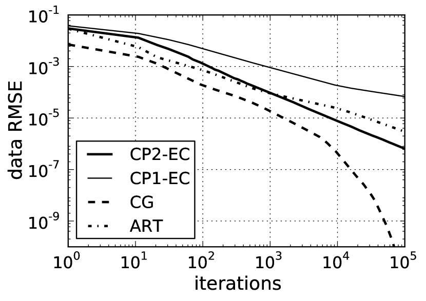
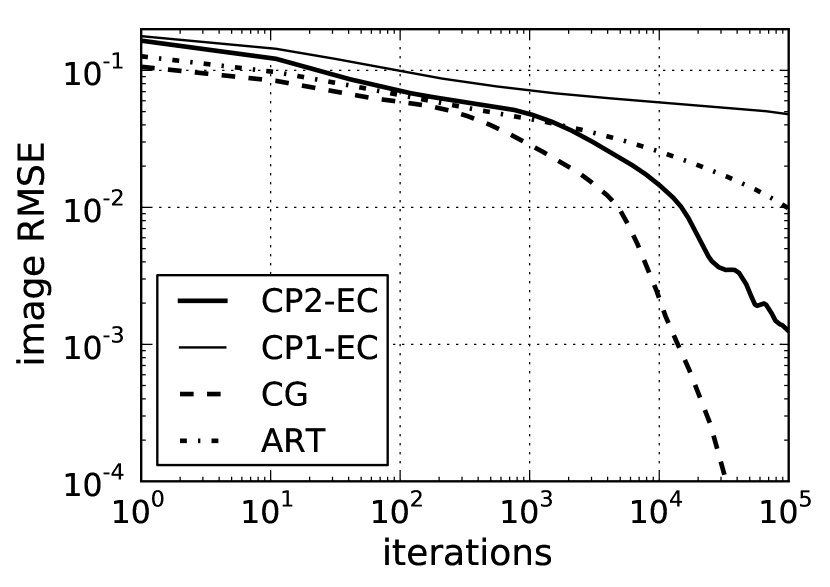
CG                                   ART

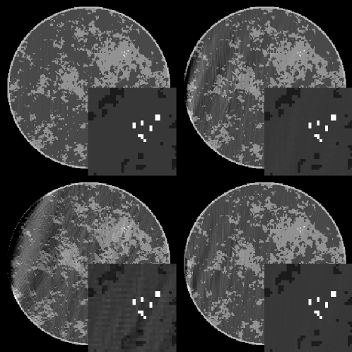
CP1-EC                               CP2-EC

Figure 4: Results of CP2-EC with ideal, simulated data. Convergence is also compared with CP1-EC, linear CG, and ART. Top row: (Left) convergence of the four algorithms in terms of data RMSE, and (Right) convergence of the four algorithms in terms of image RMSE. Bottom row: the image at iteration 10000 for CG, ART, CP Algorithm 1, and CP2-EC shown in the same gray scale as Fig. 3. The artifacts seen at the right of the images and relatively large image RMSE are indications of the poor conditioning of $\mathit{X}$. The comparison between CP2-EC and CP1-EC shows quantitatively the impact of the acceleration afforded by CP Algorithm 2.

The results of each algorithm are shown in Fig. 4. As the data are ideal, each algorithm drives the data-error to zero. The linear CG algorithm shows the smallest data RMSE, but we note similar slopes on the log-log plot of CG and CP2-EC during most of the computed iterations except near the end, where the slope of the CG curve steepens. The ART algorithm reveals a convergence slightly faster than CP2-EC, initially, but it is overtaken by CP2-EC near iteration 1000. We also note the impact of the algorithm acceleration afforded by the proposed convex feasibility framework in the comparison of CP2-EC and CP1-EC.

Because $\mathit{X}$ is designed to be left-invertible, we know also that the image estimates must converge to the breast phantom for each of the four algorithms. A similar ordering of the convergence rates is observed in the image RMSE plot, but we note that the values of the image RMSE are all much larger than corresponding values in the data RMSE plots. This stems from the poor conditioning of $\mathit{X}$, and this point is emphasized in examining the shown image estimates at iteration 10000 for each algorithm.

While the image RMSE gives a summary metric on the accuracy of the image reconstruction, the displayed images yield more detailed information on the image error incurred by truncating the algorithm iteration. The CP2-EC, CP1-EC, and ART images show wavy artifacts on the left side; the limited-angle scanning arc is over the right-side of the object. But the CG image shows visually accurate image reconstruction at the given gray scale window setting.

This initial result shows promising convergence rates for CP2-EC and that it may be competitive with existing algorithms for solving large, consistent linear systems. But we cannot draw any general conclusions on algorithm convergence, because different simulation conditions may yield different ordering of the convergence rates. Moreover, we have implemented only the basic forms of CG and ART; no attempt at pre-conditioning CG was made and the relaxation parameter of ART was fixed at 1.

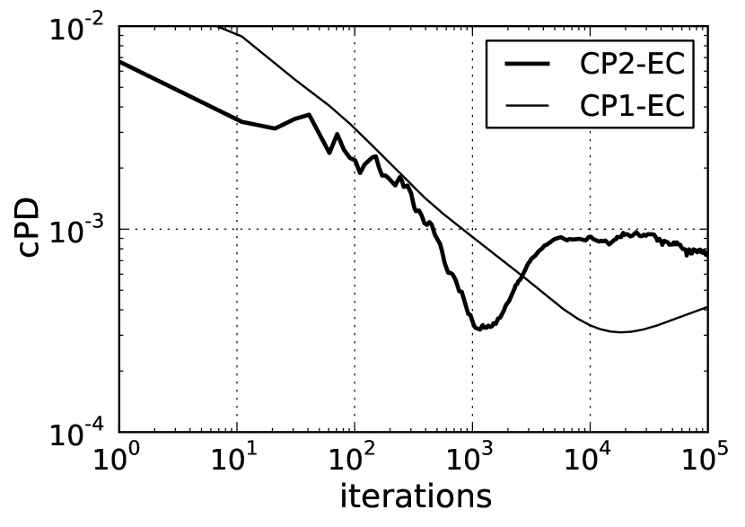
Figure 5: The conditional primal-dual gap for EC shown for CP2-EC and CP1-EC. This gap is computed by taking the difference between the primal and dual objective functions in Eqs. (11) and (12), respectively, after removing the indicator in the primal objective function: $cPD=\left|\frac{1}{2}\|\mathbf{f}-\mathbf{f}_{\text{prior}}\|^{2}_{2}+\frac{1}{2}\|X^{T}\mathbf{y}\|^{2}_{2}+\mathbf{g}^{T}\mathbf{y}-\mathbf{f}^{T}_{\text{prior}}(X^{T}\mathbf{y})\right|/\text{size}(\mathbf{f})$. The absolute value is used because the argument can be negative, and we normalize by the number of pixels $\text{size}(\mathbf{f})$ so that the primal objective function takes the form of a mean square error. The prior image $\mathbf{f}_{\text{prior}}$ for this computation is zero. The comparison between CP2-EC and CP1-EC shows quantitatively the impact of the acceleration afforded by CP Algorithm 2.

We discuss convergence in detail as it is a major focus of this article. In Fig. 5, we display the conditional primal-dual gap for the accelerated CP2-EC algorithm compared with use of CP1-EC. First, it is clear that convergence of this gap is slow for this problem due to the ill-conditionedness of $\mathit{X}$, and we note this slow convergence is in line with the image RMSE curves in Fig. 4. The image RMSE has reached only $10^{-3}$ after 10⁵ iterations. Second, the gap for CP1-EC appears to be lower than that of CP2-EC at the final iteration, but the curve corresponding to CP2-EC went through a similar dip and is returning to a slow downward trend. Third, for a complete convergence check, we must examine the constraints separately from the conditional primal-dual gap, The only constraint in EC is formulated in the indicator $\delta_{0}(\mathit{X}\mathbf{f}-\mathbf{g})$. In words, this constraint is that the given data and data estimate must be equal or, equivalently, the data RMSE must be zero. We observe in Fig. 4 that the data RMSE is indeed tending to zero. Now that we have a specific example, we reiterate the need for dividing up the convergence check into the conditional primal-dual gap and separate constraint checks. Even though the data RMSE is tending to zero, it is not numerically zero at any iteration and consequently the value of $\delta_{0}(\mathit{X}\mathbf{f}-\mathbf{g})$ is $\infty$ at all iterations. Because this indicator is part of the primal objective function in Eq. (11), this objective function also takes on the value of $\infty$ at all iterations. As a result, direct computation of the primal-dual gap does not provide a useful convergence check and we need to use the conditional primal-dual gap.

III.2 Noisy, inconsistent data and equality-constrained optimization

In this section, we repeat the previous simulation with all four algorithms except that the data now contain inconsistency modeling Poisson distributed noise. The level of the noise is selected to simulate what could be seen in a low-dose CT scan. The use of this data model contradicts the application of equality-constrained optimization and EC becomes inconsistent. But nothing prevents us from executing the CP2-EC operations, and accordingly we do so in this subsection. The linear CG algorithm can still be applied in this case, because the optimization problem in Eq. (2) is well-defined even though there is no $\mathbf{f}$ such that $\mathbf{g}=\mathit{X}\mathbf{f}$. Likewise, the linear system in Eq. (3) does have a solution even when $\mathbf{g}$ is inconsistent. The basic ART algorithm, as with CP2-EC, is not suited to this data model, because it is a solver for Eq. (1), which we know ahead of time has no solution. Again, as with CP2-EC, the steps of ART can still be executed even with inconsistent data, and we show the results here.

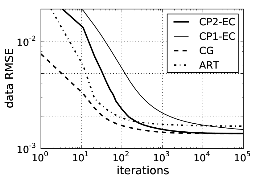
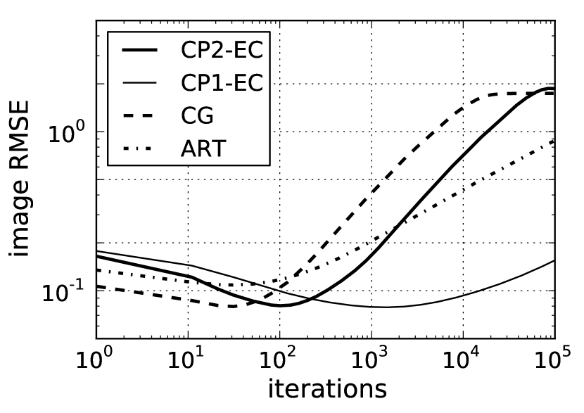
Figure 6: Metrics of CP2-EC image estimates with noisy and inconsistent, simulated data. Results are compared with CP1-EC, linear CG, and ART. Left, evolution of the four algorithms in terms of data RMSE, and right, evolution of the four algorithms in terms of image RMSE.

In Fig. 6, we show evolution plots of quantities derived from the image estimates from each of the four algorithms. Because the data are inconsistent, the data- and image-error plots have a different behavior than the previous consistent example. In this case, we know that the data RMSE cannot be driven to zero. The algorithms CP2-EC and CG converge on a value greater than zero, while CP1-EC and ART appear to need more iterations to reach the same data RMSE value.

The image RMSE shows an initial decrease to some minimum value followed by an upward trend. For CG the upward trend begins to level off at 20,000 iterations, while for CP2-EC it appears that this happens near the final 100,000th iteration. For both plots, the results of CP1-EC lag those of the accelerated CP2-EC algorithm.

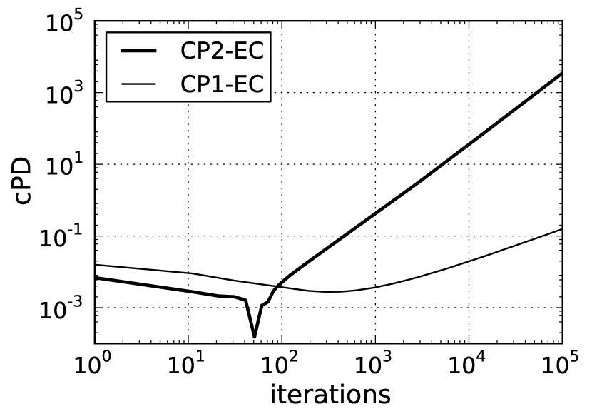
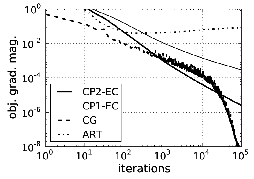
Figure 7: Convergence plots: the conditional primal-dual gap for EC (left) and the gradient magnitude of the quadratic least-squares objective function of Eq. (2) (right). The conditional primal-dual gap is only available for CP2-EC and CP1-EC, while all algorithms can be compared with the objective function gradient. The quantity cPD for this problem is explained in the caption of Fig. 5. The convex feasibility problem EC is inconsistent for the simulated noisy data, and as a result cPD diverges to $\infty$. We hypothesize that CP2-EC converges the least squares minimization problem Eq. (2), and indeed we note in the gradient plot that CP2-EC yields a decaying objective function gradient-magnitude competitive with linear CG and ART. The comparison between CP2-EC and CP1-EC shows quantitatively the impact of the acceleration afforded by CP Algorithm 2.

Turning to convergence checks, we plot the conditional primal-dual gap for EC and the magnitude of the gradient of the least-squares objective function from Eq. (2) in Fig. 7. As explained at the beginning of Sec. III, the conditional primal-dual gap tends to infinity for inconsistent convex feasibility problems because the dual objective function increases without bound. We observe, in fact, that the conditional primal-dual gap for EC is diverging - a consequence of the inconsistent data used in this simulation. In examining the objective function gradient magnitude, the curve for the CG results shows an overall convergence by this metric, because this algorithm is designed to solve the normal equations of the unregularized, least-squares problem in Eq. (2). The ART algorithm shows an initial decay followed by a slow increase. This result is not surprising, because ART is designed to solve Eq. (1) directly and not the least-squares minimization problem in Eq. (2). As an aside, we point out that in applying ART to inconsistent data it is important to allow the relaxation parameter to decay to zero. Interestingly, CP2-EC and CP1-EC show a monotonic decrease of this gradient.

The resulting gradient magnitude curves indicate convergence of the least-squares minimization, obtained by the CP algorithms. This is surprising, because the conditional primal-dual gap diverges to infinity. Indeed, the magnitude of the dual variable $\mathbf{y}_{n}$ from the algorithm listed in Fig. 1 increases steadily with iteration number. Even though the dual problem diverges, this simulation indicates convergence of the primal least-squares minimization problem in that the gradient of this objective function is observed to monotonically decrease. There is no proof that we are aware of, which covers this situation, thus we cannot claim that CP2-EC will always converge the least-squares problem. Therefore, in applying CP2-EC in this way it is crucial to evaluate the convergence criterion and to verify that the magnitude of the objective function’s gradient decays to zero. The conditional primal-dual gap cannot be used as a check for CP2-EC applied to inconsistent data.

The dependence of the gradient magnitude of the unregularized, least-squares objective function for the CP2-EC and CG algorithms is quite interesting. Between 10 and 20,000 iterations, CP2-EC shows a steeper decline in this convergence metric. But greater than 20,000 iterations the CG algorithm takes over and this metric drops precipitously. The CG behavior can be understood in realizing that the image has approximately 50,000 unknown pixel values and if there is no numerical error in the calculations, the CG algorithm terminates when the number of iterations equals the number of unknowns. Because numerical error is present, we do not observe exact convergence when the iteration number reaches 50,000, but instead the steep decline in the gradient of the least-squares objective function is observed. This comparison between CP2-EC and CG has potential implications for larger systems where the steep drop-off for CG would occur at higher iteration number.

The conditions of this particular simulation are not relevant to practical application because it is already well-known that minimizing unregularized, data-fidelity objective functions with noisy data converges to an extremely noisy image particularly for an ill-conditioned system matrix; noting the large values of the image RMSE, we know this to be the case without displaying the image. But this example is interesting in investigating convergence properties. While it is true that monitoring the gradient magnitude of the least-squares objective function yields a sense about convergence, we do not know a priori what threshold this metric needs to cross before we can say the IIR is converged, see Ref. Nonuniform_MIC for further discussion on this point related to IIR in CT. This example in particular highlights the point that an image metric of interest, such as image and data RMSE, needs to be observed to level off in combination with a steady decrease of a convergence metric. For this example, convergence of the image RMSE occurs when the gradient-magnitude of the least-squares objective function drops below $10^{-5}$, while the data RMSE convergence occurs earlier.

III.3 Noisy, inconsistent data with inequality-constrained optimization

In performing IIR with inconsistent projection data, some form of regularization is generally needed. In using the convex feasibility approach, we apply CP2-IC after deciding on the parameter $\epsilon^{\prime}$. The parameter $\epsilon^{\prime}$ has a minimum value, below which no images satisfy the data-error constraint, and larger $\epsilon^{\prime}$ leads to greater image regularity. The choice of $\epsilon^{\prime}$ may be guided by properties of the available data or a prior reconstruction. In this case, we have results from the previous section and we note that the data RMSE achieve values below 0.002. Accordingly, for the present simulation we select a tight data-error constraint $\epsilon^{\prime}=0.512$, which is equivalent to allowing a data RMSE of $\epsilon=0.002$. The CP2-IC algorithm selects the image obeying the data-error constraint closest to $\mathbf{f}_{\text{prior}}$, and to illustrate the dependence on $\mathbf{f}_{\text{prior}}$ we present results for two choices: an image of zero values, and an image set to 1 over the support of the phantom. Note that the second choice assumes prior knowledge of the object support and background value of 1. To our knowledge, there is no direct, existing algorithm for solving Eq. (13), and thus we display results for CP2-IC only. One can use a standard algorithm such as linear CG to solve the Lagrangian form of Eq. (13), but this method is indirect because it is not known ahead of time what Lagrange multiplier leads to the desired value of $\epsilon^{\prime}$.

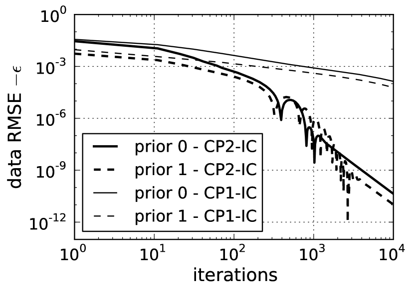
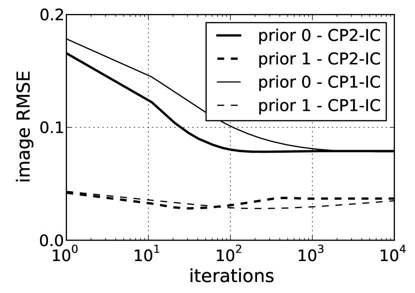
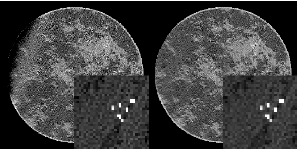
Figure 8: Results of CP2-IC and CP1-IC with noisy and inconsistent, simulated data. The curves labeled “prior 0” correspond to a zero prior image. The curves labeled “prior 1” correspond to a prior image of 1.0 on the object support. Top: (left) convergence of the data RMSE to the preset value of $\epsilon=0.002$ and (right) image RMSE. Bottom: (Left) “prior 0” final image, and (Right) “prior 1” final image. Gray scales are the same as Fig. 3. The comparison between CP2-EC and CP1-EC shows quantitatively the impact of the acceleration afforded by CP Algorithm 2.

The results of CP2-IC and CP1-IC are shown in Fig. 8. The data RMSE is seen to converge to the value established by the choice of $\epsilon^{\prime}$. In the displayed images, there is a clear difference due to the choice of prior image. The image resulting from the zero prior shows a substantial drift of the gray level on the left side of the image. Application of a prior image consisting of constant background values over the object’s true support removes this artifact almost completely. These results indicate that use of prior knowledge, when available, can have a large impact on image quality particularly for an ill-conditioned system matrix such as what arises in limited angular-range CT.

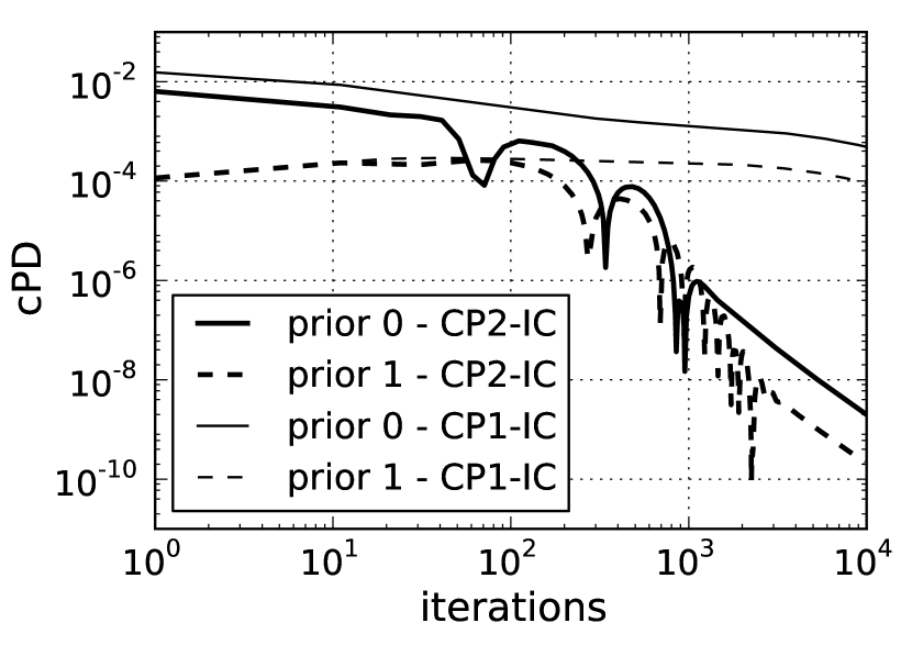
Figure 9: The conditional primal-dual gap for IC shown for CP2-IC and CP1-IC. This gap is computed by taking the difference between the primal and dual objective functions in Eqs. (13) and (14), respectively, after removing the indicator in the primal objective function: $cPD=\left|\frac{1}{2}\|\mathbf{f}-\mathbf{f}_{\text{prior}}\|^{2}_{2}+\frac{1}{2}\|X^{T}\mathbf{y}\|^{2}_{2}+\epsilon^{\prime}\|\mathbf{y}\|_{2}+\mathbf{g}^{T}\mathbf{y}-\mathbf{f}^{T}_{\text{prior}}(X^{T}\mathbf{y})\right|/\text{size}(\mathbf{f})$. The absolute value is used because the argument can be negative, and we normalize by the number of pixels $\text{size}(\mathbf{f})$ so that the primal objective function takes the form of a mean square error. The prior image $\mathbf{f}_{\text{prior}}$ for this computation is explained in the text. The comparison between CP2-IC and CP1-IC shows quantitatively the impact of the acceleration afforded by CP Algorithm 2.

Because IC in this case presents a consistent problem, convergence of the CP2-IC algorithm can be checked by the conditional primal-dual gap. This convergence criterion is plotted for CP2-IC and CP1-IC in Fig. 9. The separate constraint check is seen in the data RMSE plot of Fig. 9. We see that the accelerated version of the CP algorithm used in CP2-IC yields much more rapid convergence than CP1-IC. For example, the data RMSE constraint is reached to within $10^{-6}$ at iteration 1000 for CP2-IC, while this point is not reached for CP1-IC by even iteration 10,000. A similar observation can also be made for the conditional primal-dual gap.

III.4 Noisy, inconsistent data with two-set convex feasibility

For the last demonstration of the convex feasibility approach to IIR for limited-angular range CT, we apply CP2-ICTV, which seeks the image closest to a prior image and respects constraints on image TV and data-error. We are unaware of other algorithms, which address this problem, and only results for CP2-ICTV and CP1-ICTV are shown. In applying CP2-ICTV, we need two constants, $\epsilon^{\prime}$ and $\gamma$, and accordingly use of this algorithm is meant to be preceded by an initial image reconstruction in order to have a sense of interesting values for the data-error and image TV constraints. From the previous results, we already have information about data-error, and because we have the image estimates, we can also compute image TV values. The image TV values corresponding to the two prior image estimates differ significantly, reflecting the quite different appearance of the resulting images shown in Fig. 8. We follow the use of the support prior image, and take the corresponding value of the image TV of 4,400.

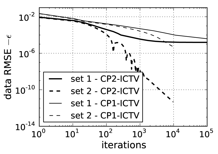
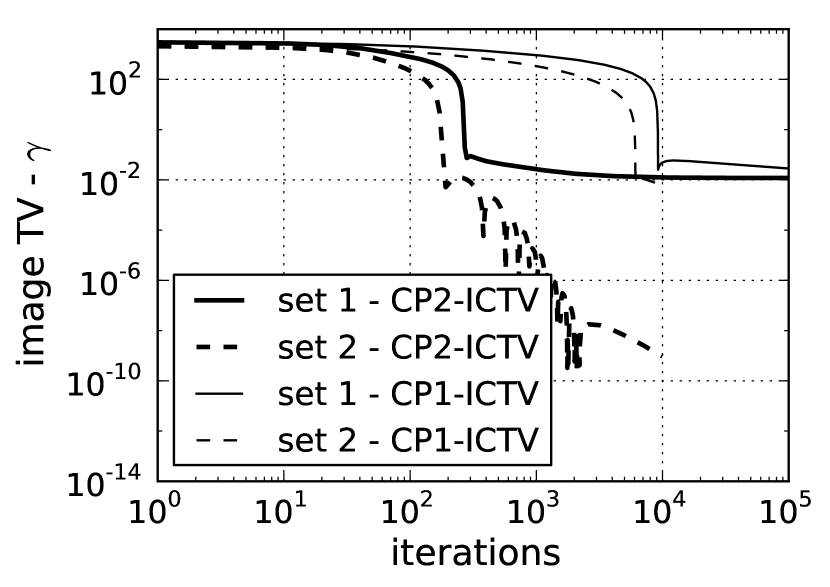
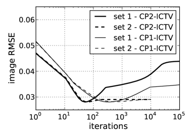
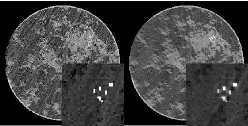
Figure 10: Results of CP2-ICTV and CP1-ICTV with noisy and inconsistent, simulated data for two different constraint set values: “set 1” refers to choosing $\epsilon^{\prime}=0.512$ (a data RMSE of $\epsilon=0.002$) and $\gamma=4000$; “set 2” refers to choosing $\epsilon^{\prime}=0.768$ (a data RMSE of $\epsilon=0.0025$) and $\gamma=3100$. Top row: (Left) evolution of data RMSE, and (Right) evolution of image TV. Middle row: evolution of image RMSE. The comparison between CP2-ICTV and CP1-ICTV shows quantitatively the impact of the acceleration afforded by CP Algorithm 2. Bottom row: (Left) resulting image of “set 1”, and (Right) resulting image of “set 2”. Gray scales are the same as Fig. 3. Note that the calculation for “set 1” is extended to $10^{5}$ iterations due to slower convergence than the results for “set 2.”

In our first example with this two-set convex feasibility problem, we maintain the tight data-error constraint $\epsilon^{\prime}=0.512$ (a data RMSE of 0.002) but attempt to find an image with lower TV by selecting $\gamma=4000$. The results for these constraint set settings, labeled “set 1”, are shown in Fig. 10. Interestingly, this set of constraints appears to be just barely infeasible; the CP2-ICTV result converges to an image TV of 4000.012 and a data RMSE of 0.00202. Furthermore, the dual variable magnitude increases steadily, an indication of an infeasible problem. The curves for image TV and data RMSE indicate convergence to the above-mentioned values, but we do not make theoretical claims for convergence of the CP algorithms with inconsistent convex feasibility problems.

In the second example, we loosen the data-error constraint to $\epsilon^{\prime}=0.768$ (a data RMSE of 0.0025) and seek an image with lower TV, $\gamma=3100$, and the results are also shown in Fig. 10. In this case, the constraint values are met by CP2-ICTV, and the resulting image has noticeably less noise than the images with no TV constraint imposed shown in Fig. 8 particularly in the ROI containing the model micro-calcifications. The image RMSE for this constraint set in ICTV is 0.029, while the comparable image RMSE from the previous convex feasibility problem, IC, with no TV constraint shown in Fig. 8 is 0.037. Thus we note a drop in image RMSE in adding the image TV constraint, but a true image quality comparison would require parameter sweeps in $\epsilon$ for IC, and $\epsilon$ and $\gamma$ for ICTV.

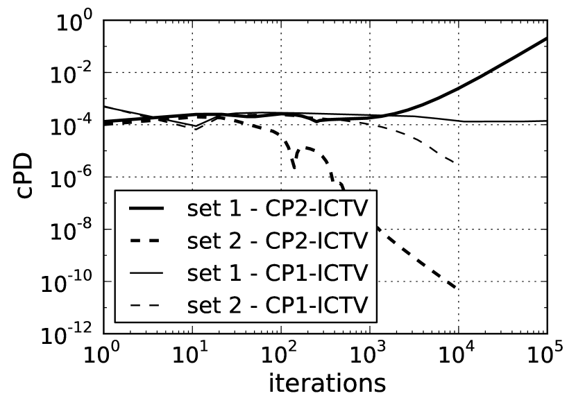
Figure 11: The conditional primal-dual gap for ICTV shown for CP2-ICTV and CP Algorithm 1. This gap is computed by taking the difference between the primal and dual objective functions in Eqs. (15) and (16), respectively, after removing the indicator in the primal objective function: $cPD=\left|\frac{1}{2}\|\mathbf{f}-\mathbf{f}_{\text{prior}}\|^{2}_{2}+\frac{1}{2}\|X^{T}\mathbf{y}\|^{2}_{2}+\epsilon^{\prime}\|\mathbf{y}\|_{2}+\gamma\|(|\mathbf{z}|)\|_{\infty}+\mathbf{g}^{T}\mathbf{y}-\mathbf{f}^{T}_{\text{prior}}(X^{T}\mathbf{y}+\nabla^{T}\mathbf{z})\right|/\text{size}(\mathbf{f})$. The absolute value is used because the argument can be negative, and we normalize by the number of pixels $\text{size}(\mathbf{f})$ so that the primal objective function takes the form of a mean square error. The prior image $\mathbf{f}_{\text{prior}}$ for this computation is explained in the text. The comparison between CP2-ICTV and CP1-ICTV shows quantitatively the impact of the acceleration afforded by CP Algorithm 2. Note that the calculation for “set 1” is extended to $10^{5}$ iterations due to slower convergence than the results for “set 2.”

Because this constraint set contains feasible solutions, the conditional primal-dual gap can be used as a convergence check for CP2-ICTV. This gap is shown for both sets of constraints in Fig. 11. For CP2-ICTV there is a stark contrast in behavior between the two constraint sets. The feasible set shows rapid convergence, while the infeasible set show no decay in the conditional primal-dual gap below 1000 iterations and a steady increase from 1000 to 10,000 iterations. Again, the accelerated CP algorithm used in CP2-ICTV yields a substantially faster convergence rate than CP1-ICTV for this example.

III.5 Comparison of algorithms

With the previous simulations, we have illustrated use of the convex feasibility framework on EC, IC, and ICTV for IIR in CT. The example for EC serves the purpose of demonstrating convergence properties of CP2-EC on the ubiquitous least-squares minimization and establishing that this algorithm has competitive convergence rates with standard algorithms, linear CG and ART. We do note that CG, on the shown example, does have the fastest convergence rate, but the difference in convergence rate between CP2-EC, CG, and ART is substantially less than their gap with the basic CP1-EC. For convex feasibility problems IC and ICTV, we have optimization problems where the current methodology can be easily adapted to solve, but the standard algorithms linear CG and ART cannot easily be applied. Because we have the comparisons of the CP algorithms on the EC simulations and because we have seen convergence competitive with linear CG and ART, we speculate that CP2-IC and CP2-ICTV have competitive convergence rates with any modification of CG or ART that could be applied to IC and ICTV. In short, the convex feasibility framework using CP Algorithm 2 provides a means for proto-typing a general class of optimization problems for IIR in CT, while having convergence rates competitive with standard, but more narrowly applicable, large-scale solvers. Furthermore, concern over algorithm convergence is particularly important for ill-conditioned system models such as those that arise in limited angular-range CT scanning.

Convex feasibility presents a different design framework than unconstrained minimization or mixed optimizations, combining e.g. data-fidelity objective functions with constraints. For example, the field of compressed sensing (CS) candes2008introduction has centered on devising sparsity exploiting optimization for reduced sampling requirements in a host of imaging applications. For CT, in particular, exploiting gradient magnitude sparsity for IIR has garnered much attention, requiring the solution to constrained, TV-minimization sidky2008image ; SidkyCP:2012 or TV-penalized, least-squares Jensen2011 ; Defrise:11 ; fessler:2012 ; SidkyCP:2012 . The convex feasibility, ICTV, involves the same quantities but can be used only indirectly for a CS-style optimization; the data-error can be fixed and multiple runs with CP2-ICTV for different $\gamma$ can be performed with the goal of finding the minimum $\gamma$ given the data and fixed-$\epsilon$. On the other hand, due to the fast convergence of CP2-ICTV it may be possible to perform the necessary search over $\gamma$ faster than use of an algorithm solving constrained, TV-minimization or a combined unconstrained objective function. Also, use of ICTV provides direct control over the physical quantities in the optimization problem, image TV and data-error, contrasting with the use of TV-penalized, least-squares, where there is no clear connection between the smoothing parameter $\alpha$ and the final image TV or data-error. In summary, ICTV provides an alternative design for TV-regularized IIR.

IV Conclusion

We have illustrated three examples of convex feasibility problems for IIR applied to limited angular-range CT, which provide alternative designs to unconstrained or mixed optimization problems formulated for IIR in CT.

One of the motivations of the alternative design is that these convex feasibility problems are amenable to the accelerated CP algorithm, and the resulting CP2-EC, CP2-IC, and CP2-ICTV algorithms solve their respective convex feasibility problems with a favorable convergence rate– an important feature for the ill-conditioned data model corresponding the limited angular-range scan. The competitive convergence rate is demonstrated by comparing convergence of CP2-EC with known algorithms for large-scale optimization. We then note that CP2-IC and CP2-ICTV, for which there is no alternative algorithm that we know of, appears to have similar convergence rates to CP2-EC.

Aside from the issue of convergence rate, algorithm design can benefit from the different point of view offered by convex feasibility. For imaging applications this design approach extends naturally to considering non-convex feasibility sets luke2005relaxed ; Han:2012 , which can have some advantage particularly for very sparse data problems. Future work will consider extension of the presented methods to the non-convex case and application of the present methods to actual data for CT acquired over a limited angular-range scan.

Appendix A Pseudocode for CP2-ICTV

The pseudocode for CP2-ICTV appears in Fig. 12, and we explain variables not appearing in Secs. II.5.1 and II.5.2. At Line 6 the symbol $\nabla$ represents a numerical gradient computation, and it is a matrix which applies to an image vector and yields a spatial-vector image, where the vector at each pixel/voxel is either 2 or 3 dimensional depending on whether the image reconstruction is being performed in 2 or 3 dimensions. Similarly, the variables $\mathbf{t}$ and $\mathbf{z}_{n}$ are spatial-vector images. At Line 7 the operation “$|\cdot|$” computes the magnitude at each pixel of a spatial-vector image, accepting a spatial-vector image and yielding a scalar image. This operation is used, for example, to compute a gradient-magnitude image from an image gradient. The ratio appearing inside the square brackets of Line 7 is to be understood as a pixel-wise division yielding a scalar image. It is possible that at some pixels the numerator and denominator are both zero in which case we define $0/0=1$. The quantity in the square brackets evaluates to a scalar image, which then multiplies a spatial-vector image; this operation is carried out, again, in pixel-wise fashion where the spatial-vector at each pixel of $\mathbf{t}$ is scaled by the corresponding pixel-value. At Line 8, $\nabla^{T}$ is the transpose of the matrix $\nabla$, see Ref. SidkyCP:2012 for one possible implementation of $\nabla$ and $\nabla^{T}$ for two dimensions.

1:$L\leftarrow\|(\mathit{X},\nabla)\|_{2};\;\tau\leftarrow 1;\;\sigma\leftarrow 1/L^{2};\;n\leftarrow 0$

2:initialize $\mathbf{f}_{0}$, $\mathbf{y}_{0}$, and $\mathbf{z}_{0}$ to zero vectors

3:$\bar{\mathbf{f}}_{0}\leftarrow\mathbf{f}_{0}$

4:repeat

5:     $\mathbf{y}^{\prime}_{n}\leftarrow\mathbf{y}_{n}+\sigma(\mathit{X}\bar{\mathbf{f}}_{n}-\mathbf{g})$; $\;\mathbf{y}_{n+1}\leftarrow\max(\|\mathbf{y}^{\prime}_{n}\|_{2}-\sigma\epsilon^{\prime},0)\frac{\mathbf{y}^{\prime}_{n}}{\|\mathbf{y}^{\prime}_{n}\|_{2}}$

6:     $\mathbf{t}\leftarrow\mathbf{z}_{n}+\sigma\nabla\mathbf{f}_{n}$

7:     $\mathbf{z}_{n+1}\leftarrow\mathbf{t}\,\left[\left(|\mathbf{t}|-\sigma\,\text{proj}_{\text{Diamond}(\gamma)}(|\mathbf{t}|/\sigma)\right)/|\mathbf{t}|\right]$

8:     $\mathbf{f}_{n+1}\leftarrow\left[\mathbf{f}_{n}-\tau(\mathit{X}^{T}\mathbf{y}_{n+1}-\mathbf{f}_{\text{prior}}+\nabla^{T}\mathbf{z}_{n+1})\right]/(1+\tau)$

9:     $\theta\leftarrow 1/\sqrt{1+2\tau}$; $\tau\leftarrow\tau\theta$; $\sigma\leftarrow\sigma/\theta$

10:     $\bar{\mathbf{f}}_{n+1}\leftarrow\mathbf{f}_{n+1}+\theta(\mathbf{f}_{n+1}-\mathbf{f}_{n})$

11:     $n\leftarrow n+1$

12:until $n\geq N$

Figure 12: Pseudocode for $N$ steps of the accelerated CP algorithm instance for solving Eq. (15) with parameters $\epsilon^{\prime}$ and $\gamma$. Variables are explained in the text, and pseudocode for the function $\text{proj}_{\text{Diamond}(\gamma)}(\mathbf{x})$ is given in Fig. 13.

The pseudocode for the function $\text{proj}_{\text{Diamond}(\gamma)}(\mathbf{x})$ appears in Fig. 13. This function is essentially the same as what is listed in Figure 1 of Ref. duchi2008efficient ; we include it here for completeness. The “if” statement at Line 2, checks if the input vector $\mathbf{x}$ is already in $\text{Diamond}(\gamma)$. Also, because the function $\text{proj}_{\text{Diamond}(\gamma)}(\mathbf{x})$ is used with a non-negative vector argument in Line 7 of Fig. 12, the multiplication by $\text{sign}(\mathbf{x})$ at the end of the algorithm in Fig. 13 is unnecessary for the present application. But we include this $\text{sign}(\mathbf{x})$ factor so that the function applies to any $N$-dimensional vector.

1:function $\text{proj}_{\text{Diamond}(\gamma)}$($\mathbf{x}$)

2:     if $\|\mathbf{x}\|_{1}\leq\gamma$ then

3:         return $\mathbf{x}$

4:     end if

5:     $\mathbf{m}=|\mathbf{x}|$

6:     Sort $\mathbf{m}$ in descending order: $m_{1}\geq m_{2}\geq\dots m_{N}$

7:     $\rho\leftarrow\max j$ such that $m_{j}-\frac{1}{j}\left(\sum_{k=1}^{j}m_{k}-\gamma\right)>0$, for $j\in[1,N]$

8:     $\theta\leftarrow(1/\rho)\left(\sum_{k=1}^{\rho}m_{k}-\gamma\right)$

9:     $\mathbf{w}=\max(|\mathbf{x}|-\theta,0)$

10:     return $\mathbf{w}\,\text{sign}(\mathbf{x})$

11:end function

Figure 13: Pseudocode for the function $\text{proj}_{\text{Diamond}(\gamma)}(\mathbf{x})$, which projects $\mathbf{x}$ onto the $\ell_{1}$-ball of scale $\gamma$. This function appears at line 7 of algorithm in Fig. 12. The vector $\mathbf{x}$ is taken to be one-dimensional with length $N$, and the individual components are labeled $x_{i}$ with index $i$ being an integer in the interval $[1,N]$.

References

- (1) R. Gordon, R. Bender, and G. T. Herman, “Algebraic reconstruction techniques (ART) for three-dimensional electron microscopy and X-ray photography,” J. Theor. Biol. 29, 471–481, (1970).
- (2) G. T. Herman, Image Reconstruction from Projections, New York: Academic, 1980.
- (3) T. L. Jensen, J. H. Jørgensen, P. C. Hansen, and S. H. Jensen, “Implementation of an optimal first-order method for strongly convex total variation regularization,” BIT Num. Math. 52, 329–356, (2012).
- (4) M. Defrise, C. Vanhove, and X. Liu, “An algorithm for total variation regularization in high-dimensional linear problems,” Inv. Prob. 27, 065002, (2011).
- (5) S. Ramani and J. Fessler, “A splitting-based iterative algorithm for accelerated statistical X-ray CT reconstruction,” IEEE Trans. Med. Imag. 31, 677–688, (2012).
- (6) E. Y. Sidky, J. H. Jørgensen, and X. Pan, “Convex optimization problem prototyping for image reconstruction in computed tomography with the Chambolle-Pock algorithm,” Phys. Med. Biol. 57, 3065–3091, (2012).
- (7) P. Combettes, “The convex feasibility problem in image recovery,” Adv. Imag. Electron Phys. 95, 155–270, (1996).
- (8) P. L. Combettes, “The foundations of set theoretic estimation,” IEEE Proc. 81, 182–208, (1993).
- (9) X. Han, J. Bian, E. L. Ritman, E. Y. Sidky, and X. Pan, “Optimization-based reconstruction of sparse images from few-view projections,” Phys. Med. Biol. 57, 5245–5274, (2012).
- (10) A. Chambolle and T. Pock, “A first-order primal-dual algorithm for convex problems with applications to imaging,” J. Math. Imag. Vis. 40, 120–145, (2011).
- (11) A. C. Kak and M. Slaney, Principles of Computerized Tomographic Imaging, New York: IEEE Press, 1988.
- (12) J. H. Jørgensen, E. Y. Sidky, and X. Pan, “Quantification of admissible undersampling for sparsity-exploiting iterative image reconstruction in X-ray CT,” IEEE Trans. Med. Imaging 32, 460–473, (2013).
- (13) J. Nocedal and S. Wright, Numerical Optimization, 2nd ed., Springer, 2006.
- (14) C. C. Paige and M. A. Saunders, “LSQR: an algorithm for sparse linear equations and sparse least squares,” ACM Trans. Math. Soft. 8, 43–71, (1982).
- (15) R. T. Rockafellar, Convex analysis, Princeton Univ. Press, 1970.
- (16) T. Pock and A. Chambolle, “Diagonal preconditioning for first order primal-dual algorithms in convex optimization,” in International Conference on Computer Vision (ICCV 2011), 2011, 1762–1769.
- (17) Y. Nesterov, “A method of solving a convex programming problem with convergence rate O(1/),” in Soviet Mathematics Doklady, 27, no. 2, 1983, 372–376.
- (18) A. Beck and M. Teboulle, “Fast gradient-based algorithms for constrained total variation image denoising and deblurring problems,” IEEE Trans. Imag. Proc. 18, 2419–2434, (2009).
- (19) J. H. Jørgensen, E. Y. Sidky, and X. Pan, “Ensuring convergence in total-variation-based reconstruction for accurate microcalcification imaging in breast X-ray CT,” in Nuclear Science Symposium and Medical Imaging Conference (NSS/MIC), 2011 IEEE, Valencia, Spain, 2011, 2640–2643.
- (20) C. Vogel, Computational methods for inverse problems, Society for Industrial Mathematics, 2002, 23.
- (21) J. Duchi, S. Shalev-Shwartz, Y. Singer, and T. Chandra, “Efficient projections onto the -ball for learning in high dimensions,” in Proceedings of the 25th international conference on Machine learning, ICML, 2008, 272–279.
- (22) J. H. Jørgensen, P. C. Hansen, E. Y. Sidky, I. S. Reiser, and X. Pan, “Toward optimal X-ray flux utilization in breast CT,” in Proceedings of the 11th International Meeting on Three-Dimensional Image Reconstruction in Radiology and Nuclear Medicine, 2011, arxiv preprint arxiv:1104.1588 (http://arxiv.org/abs/1104.1588).
- (23) I. Reiser and R. M. Nishikawa, “Task-based assessment of breast tomosynthesis: Effect of acquisition parameters and quantum noise,” Med. Phys. 37, 1591–1600, (2010).
- (24) H. H. Barrett and K. J. Myers, Foundations of Image Science, Hoboken, NJ: John Wiley & Sons, 2004.
- (25) E. J. Candès and M. B. Wakin, “An introduction to compressive sampling,” IEEE Signal Process. Mag. 25, 21–30, (2008).
- (26) E. Y. Sidky and X. Pan, “Image reconstruction in circular cone-beam computed tomography by constrained, total-variation minimization,” Phys. Med. Biol. 53, 4777–4807, (2008).
- (27) D. R. Luke, “Relaxed averaged alternating reflections for diffraction imaging,” Inv. Prob. 21, 37–50, (2005).