Traversing Cosmological Singularities
Complete Journeys Through Spacetime Including Antigravity 111Invited
article, to appear in Beyond the Big Bang, Competing Scenarios for an
Eternal Universe, Ed. Rudy Vaas, ISBN 978-3-540-71422-4,
http://www.springer.com/astronomy/general+relativity/book/978-3-540-71422-4 .
Abstract
A unique description of the Big Crunch-Big Bang transition is given at the classical gravity level, along with a complete set of homogeneous, isotropic, analytic solutions in scalar-tensor cosmology, with radiation and curvature. All solutions repeat cyclically; they have been obtained by using conformal gauge symmetry (Weyl symmetry) as a powerful tool in cosmology, and more generally in gravity. The significance of the Big Crunch-Big Bang transition is that it provides a model independent analytic resolution of the singularity, as an unambiguous and unavoidable solution of the equations at the classical gravitational physics level. It is controlled only by geometry (including anisotropy) and only very general features of matter coupled to gravity, such as kinetic energy of a scalar field, and radiation due to all forms of relativistic matter. This analytic resolution of the singularity is due to an attractor mechanism created by the leading terms in the cosmological equation. It is unique, and it is unavoidable in classical relativity in a geodesically complete geometry. Its counterpart in quantum gravity remains to be understood.
I Introduction and Summary of Results
Resolving the big bang singularity is one of the central challenges for fundamental physics and cosmology. The issue arises naturally in the context of classical relativity due to the geodesically incomplete nature of the singular spacetime hawking1 -hawkPenrose . The resolution may not be completed until the physics is understood in the context of quantum gravity. String theory or other forms of quantum gravity have not yet reached the technical level to tackle this cosmological issue. Solutions in the classical theory of relativity coupled to a scalar field are directly connected to the quantum theory in the context of string theory, where the classical field theory solution provides a critical string background consistent with perturbative worldsheet conformal symmetry. Therefore analytic solutions obtained in the classical theory of relativity, and insights on geodesic completeness with the resolution of the singularity, are relevant not only for the classical theory but also contribute to the quantum treatment. Indeed such classical solutions may well guide the future development of the quantum theory of gravity as applied to cosmology.
In recent papers with Shih-Hung Chen, Paul Steinhardt and Neil Turok inflation-BC -BCST2 , I studied a model of a scalar field minimally coupled to gravity, with some specific forms of potential energy for the scalar field, and included curvature and radiation as two additional parameters. Our goal was to obtain analytically the complete set of configurations of a homogeneous and isotropic universe as a function of time. This led to a geodesically complete description of the universe, including the passage through the cosmological singularities, at the classical level. We gave all the solutions analytically without any restrictions on the parameter space of the model or initial values of the fields.
The overall approach in this investigation was in contrast to specific analytic, approximate, or numerical solutions that are usually fine tuned from the point of view of initial conditions and/or the potential energy function for the scalar field, to force a solution in which the universe has a particular desired behavior as motivated by prejudices and observations. Instead, we aimed at the global structure of solution space that can emerge from a class of theories, so that we can gain a better understanding of how the features of our own universe could emerge. Indeed we learned important general lessons that transcend the specific forms of potentials we could analyze analytically.
We found that geodesic completeness together with anisotropy of spacetime play very significant roles in understanding the phenomena in the vicinity of the Big Bang or Big Crunch singularities, and the transition between them, which involves a brief period of antigravity. Therefore it is important to describe the entire set of geodesically complete analytic solutions first in the absence of anisotropy and then their modification in the presence of anisotropy.
In the absence of anisotropy, we could solve the equations fully only for some forms of the potential energy of the scalar field, but this was sufficient to extract general lessons that would apply to a much wider class of models. An essential ingredient was the requirement of a geodesically complete geometry. The complete set of exact solutions, combined with conformal symmetry, provided the ingredients to construct the geodesically complete geometry. Then we learned that for generic solutions (meaning no restrictions on initial conditions or parameters of the model), the universe goes through a singular (zero-size) bounce by entering a period of antigravity at each big crunch and exiting from it at the following big bang. This happens cyclically without violating the null energy condition (Fig.2a). There is a special subset of geodesically complete non-generic solutions which perform zero-size bounces without entering the antigravity regime in all cycles. For these, initial values of the fields are synchronized and quantized but the parameters of the model are not restricted (Figs.4-7). There is also a subset of spatial curvature-induced solutions that have finite-size bounces in the gravity regime and never enter the antigravity phase (Figs.8,9). These exist only within a small continuous domain of parameter space without fine tuning initial conditions. To obtain these results, we identified 25 regions of a 6-parameter space in which the complete set of analytic solutions were explicitly obtained.
In the presence of anisotropy, all solutions mentioned above are strongly modified near the singularity (see Figs.2b,3). An attractor mechanism pulls the solution to a particular region of the phase space of the degrees of freedom (scalar and tensor fields). The dominant terms in the cosmological equations are the anisotropy of the geometry, and the kinetic energy of the scalar field, while “radiation” due to all species of relativistic particles is the next most important ingredient. Other terms, such as inhomogeneities, massive matter, potential energy, cosmological constant, etc. are all subdominant near the singularity. In particular, since the potential energy of the scalar field is negligible (unless it has non-typical behavior near the singularity), the resolution of the singularity described here is essentially model independent. With only the dominant terms just mentioned, we discovered a new phenomenon which is unambiguous classical evolution through cosmological singularities, as well as generic in geodesically complete spacetimes. This is the attractor mechanism that modifies all the solutions described in the previous paragraph, irrespective of their initial conditions, such that it ensures the generic and special solutions to undergo a big crunch/big bang transition by contracting to zero size, passing only through the origin of field space (see figures) to enter a brief antigravity phase, shrinking to zero size again, and re-emerging into an expanding normal gravity phase, again by passing only through the origin of field space, as in Figs.2b,3. The origin of field space is then dynamically forced to be a natural initial condition for all scalar fields at the Big Bang.
This result of the attractor can be used as an unavoidable initial condition for all scalar fields, including the dilaton of string theory, the Higgs field, or other scalar fields, in order to discuss their cosmological history. In fact, based on this observation, the history of the Higgs field is currently under construction BCST3 . Similarly, this may be useful for the construction of complete cosmologies like the inflation model inflationGuth -SciAm , the cyclic model cyclic1 -Rendall , or a hybrid model that combines the attractive features of both scenarios.
New tools to obtain analytic solutions of the Friedmann equations used in our work came from Two-Time Physics (2T-physics) that was developed since 1995 (for a recent summary see 2TPhaseSpace ). Although the full machinery of 2T-physics is not needed for this cosmological application (only familiar conformal symmetry in 3+1 dimensions is enough), it is important to emphasize that the techniques and physical clues were first developed in the context of 2T-physics. The more powerful aspects of the 2T approach are also expected to become relevant in a variety of applications in physics. For this reason I give a brief introduction of 2T-physics in the following section, and then concentrate on the relevant local scaling symmetry directly in 3+1 dimensions in the sections after that.
II Basic Principles of 2T-Physics
In this section I explain how the local scaling symmetry (Weyl symmetry Weyl ) essential in our cosmological application emerges from a deep principle of physics and how local scaling symmetry in cosmology is an example of much broader hidden symmetries and dualities that are made manifest by 2T-physics as properties of a higher spacetime.
This section is included for two reasons. The first is to explain the historical development of the ideas/methods, including the Weyl symmetry, that ended up being useful in cosmology. The second, and more important reason is to emphasize the richness of the underlying formulation that is waiting to be applied to broad areas of physics. To understand the rest of the paper it is not essential to digest the contents of this section (so the impatient reader could skip to the next section).
2T-physics is a dimensional reformulation of physics in 3+1 dimensions. It applies universally and correctly to all macroscopic or microscopic phenomena at classical and quantum levels. It can be used to shed new light on, and develop new computational methods in, well established fields of physics, or it can be applied as a new guiding unification principle to formulate and explore lesser known areas of physics, such as M-theory.
More generally, 2T-physics is formulated in space and time dimensions. Note that in contrast to the 6 or 7 additional spatial extra dimensions in string/M-theory, which usually are compactified, the extra 1+1 dimensions in 2T-physics are distinguished and not small. Thus, the 2T version of M-theory would have a total of 13 dimensions. In fact, initially, 2T-physics emerged from my observation that the extended supersymmetry of M-theory is actually a SO covariant 12-dimensional supersymmetry written in disguise in an 11-dimensional basis (this 2-time signal in M-theory is distinct and prior to F-theory which extended M-theory to 12 dimensions). This prompted the development of S-theory in dimensions in 1996, which was an algebraic unification of the supersymmetries of the various corners of M-theory within the supergroup OSp, which in turn led to 2T-physics after a few twists and turns by 1998 (see 2TPhaseSpace for references on these developments). A complete set of references and an elementary explanation of 2T-physics is given in ExtraDims .
The elementary notions of 2T-physics in 1998, which were formulated in phase space (position and momentum), evolved by now into a new principle of physics: observer independence in phase space 2TPhaseSpace . This principle generalizes a similar notion championed by Albert Einstein who, with his general coordinate symmetry, showed us how to formulate physics in a way that the basic laws are independent of the status of observers is coordinate space. The new principle takes this notion one step further into phase space, since, after all, observers are defined with not only position but also momentum. The stronger gauge symmetry at the base of 2T-physics, phase space gauge symmetry, goes beyond general covariance, or Yang-Mills type gauge symmetries in position space, and explores gauge symmetry in phase space that covers a much larger class of observers. As a consequence, 2T-physics comes with a lot more gauge symmetry as compared to 1T-physics, and this guides us to a more fundamental and unified form of the laws of physics, that is independent of the bias of observers in phase space.
To be able to realize the phase space gauge symmetry, an extra space and an extra time dimension must be added. The reason is that, in a spacetime with only one time dimension, phase space gauge symmetry is too strong and reduces the system to trivial content in the gauge invariant physical subspace. With an extra 1-space and 1-time dimensions the desired gauge symmetry is realizable and yields very rich content. Consequently, the difference between 2T-physics in dimensions and 1T-physics in 3+1 dimensions is only gauge degrees of freedom. That is, there are no Kaluza-Klein degrees of freedom that fill the gap between 3+1 and . Instead, the available physical degrees of freedom (in the gauge invariant subspace) effectively describe 3+1 dimensional holographic “shadows” of the phenomena that have a more unified and more symmetric description in the full dimensions.
To help grasp the relation between 1T-physics and 2T-physics, I suggested a metaphor (see Fig.3 in 2TPhaseSpace ). Consider the many possible shadows of a 3 dimensional object projected from different perspectives on the surrounding walls of a 3-dimensional room. A flatlander that can crawl and measure only on the surface of the walls would think that the shadows of different shapes are different “beasts” and move differently. Similarly, even though according to 2T-physics a unique dynamical system in dimensions generates a large variety of 1-time “shadows”’, 1T-physics presents these “shadows” in 3+1 dimensional space-times as different dynamical systems in terms of different Hamiltonians (different times). In this way 1T-physics misses the underlying relationship between the “shadows” as well as the underlying properties (e.g. symmetries) of the higher dimensional space-time. Actually, it turns out that each “shadow” is a holographic image that retains all the information of the d+2 structure. This information takes the form of hidden symmetries, dualities and other non-trivial structures, which are hard to notice by the 1T physicist that investigates the “shadows” (i.e. different dynamical systems).
The advantage is that, the higher dimensions, that include the gauge degrees of freedom, provide multiple new perspectives in higher spacetime (observers in phase space) in which to view 3+1 dimensional phenomena with more clarity and unity. This is somewhat analogous to Einstein’s observers in relativistic 4-dimensional spacetime whose very different views of physical phenomena from their own perspectives in spacetime (defined by gauge choices) are united by the underlying gauge symmetries that elevate time to the same level of importance as space in the formulation of fundamental laws of physics. Similarly, with phase space gauge symmetry, all components of momentum and position (including time and Hamiltonian) are all at the same level of importance in the formulation of fundamental laws of physics. In this way, as in the case of Einstein’s surprising conclusions, 2T-physics makes numerous surprising predictions of previously unknown dualities and hidden symmetries in 1T-physics, as natural consequences of the underlying phase space gauge symmetry and global symmetry in dimensions. The dimensional equations unite diverse dynamical systems in 3+1 dimensions (diverse Hamiltonians used by diverse 1T observers in 3+1 dimensional phase space) and give them a single unified higher dimensional interpretation.
2T-physics is causal (no time-like closed loops or grandfather paradoxes), and it is unitary (free of ghosts), due to the gauge symmetry, and describes physics correctly at all levels of distance or energy. It has been developed in the realms of classical or quantum particles with interactions, their twistor equivalents, field theory including the Standard Model, gravity, supergravity and high spin fields.
SO global symmetry, and its local extension, is the natural spacetime symmetry of the ambient dimensional flat spacetime for 2T-physics (more generally d+2, if small compactified dimensions are included, as in string theory). This global symmetry in dimensions takes the form of conformal symmetry SO in 3+1 dimensions in the case of massless systems, as well as the little known hidden symmetry of many other systems, such as the Friedmann-Lemaître-Robertson-Walker (FLRW) universe, the hydrogen atom, and numerous other cases (see Fig.1 in 2TPhaseSpace ). This comes about as follows.
The 2T theory, in any of its forms mentioned above (particles, field theory, twistors, etc.), may be gauge fixed from to 3+1 in many possible ways, such that each gauge choice corresponds to the perspective of an observer in 3+1 dimensional phase space as embedded in . It is evident that there are an infinite number of ways in which 3+1 dimensional phase space sits within dimensional phase space (the extra phase space in 1+1 dimensions is gauge degrees of freedom). Each such perspective provides a “shadow” of the phenomena in dimensions as seen by an observer using that 3+1 phase space perspective. All such observers are related to each other by canonical transformations in 3+1 dimensions, where such transformations are gauge transformations in the 2T-physics formalism. Any global symmetry (such as SO, or other global symmetry in a specific model in ), that commutes with the gauge symmetry, remains unspoiled in all shadows. This is similar to the global Lorentz symmetry that remains as a hidden symmetry in Maxwell’s electro-magnetism or any Yang-Mills theory when one chooses a gauge, such as the Coulomb gauge. Thus, all shadows share the same global symmetry inherited from dimensions, while all shadows are related to each other by dualities since (being gauge choices) they all are holographic representations of the same parent theory in dimensions.
The richness (and usefulness) of 2T-physics is in its ability to unify the diverse forms of 1T-physics as perceived in various shadows and in establishing previously unknown dualities and hidden symmetries that are implemented via canonical transformations among shadows. This predicted additional information that relates “shadows” to each other is missing systematically in 1T-physics (although some such cases could, and have been, accidentally discovered within 1T-physics). The applications of this new systematic concepts, for example, to develop new computational tools in 1T-physics, or to gain deeper insight into spacetime and physics, are still largely underdeveloped.
There is a particular perspective (gauge choice) called the “conformal shadow” in which the linear SO Lorentz symmetry in flat dimensions is perceived by the corresponding observer in 3+1 dimensions as the familiar conformal symmetry of 3+1 dimensions. Most work in 2T-physics has concentrated on the conformal shadow because it is then possible to connect to the familiar formalism of relativistic field theory used in particle physics and gravity. Then it is possible to interpret the familiar conformal symmetry as one perspective in which to view the phenomena in dimensions. Although this is a very useful perspective to connect to familiar language, other perspectives would provide additional information about the underlying unity in the form of dual versions of the same theory that may be used both as computational tools as well as for deeper insights into spacetime and the corresponding physics.
The cosmological application discussed in this paper emerged from the analysis of 2T-gravity 2Tgravity in the conformal shadow 2TgravityGeometry . A necessary consequence of 2T-gravity is that the emergent 1T-gravity in 3+1 dimensions must come with an additional local scaling symmetry, known as Weyl symmetry, realized in a specific form. This is possible but not required in 1T field theory. This local scaling symmetry is a remnant of general coordinate reparameterization symmetry in dimensions; specifically, it is reparameterizations of the extra 1+1 dimensions locally at each point of the 3+1 dimensions 2TgravityGeometry . To the observer in the conformal shadow, the Weyl symmetry must be present as an essential property of gravity and all the degrees of freedom that couple to it. Making a gauge choice for the Weyl symmetry amounts to choosing the observer’s coordinates in the extra 1-space and 1-time dimensions.
To summarize, the connection of 2T-physics to conformal symmetry is dictated by the phase space gauge symmetry. This underlying gauge symmetry requires dimensions (more gerally The spacetime symmetries in dimensions that commute with the gauge symmetry, such as the linear SO in flat dimensional spacetime, remains as a hidden symmetry in all shadows. In the particular shadow called the conformal shadow, the hidden SO takes the form of the non-linearly realized conformal SO transformations in 3+1 dimensions. In curved spacetime the symmetry includes general coordinate transformations of all coordinates. In the conformal shadow, at each 3+1 dimensional point, the reparametrizations of the extra 1+1 dimensions take the form of local scaling transformations, which is the Weyl transformation. Thus, 2T-physics requires that all 3+1 dimensional physics must be formulated in a Weyl symmetric formalism, whose form is already predicted by the structure of the dimensional approach.
From this point on, using only 3+1 dimensional field theory methods, and requiring the Weyl symmetry, is sufficient to proceed without further guidance from 2T-physics. The Weyl symmetry plays multiple roles: (i) it restricts the terms that are allowed in the gravitational action and matter couplings, (ii) it is used as a tool for solving the well known cosmological equations of Einstein’s theory by taking advantage of various gauge choices (a super simplified example of the observers, shadows and dualities mentioned above), (iii) it is a guide for completing the geometry geodesically.
III Using the Weyl Symmetry to Solve Cosmological Equations
The Weyl symmetry does not allow any dimensionful parameters in the action that describes the coupling of gravity and matter fields. Here is the action, the Lagrangian density, and the determinant of the metric In particular, the usual Einstein-Hilbert term is not permitted since it contains a dimensionful parameter. However, what is permitted is conformally coupled scalars deser as well as the usual gravitational coupling to fermions and gauge fields. A full theory that includes the Standard Model or its supersymmetric or grand unified extensions, and their coupling to gravity, including a mass generating mechanism for the Higgs field consistent with Weyl symmetry, can be constructed. Indeed this was done directly in dimensions 2tStandardModel 2tSM2 , and its conformal shadow is precisely the emergent Weyl invariant theory in 3+1 dimensions.
For the purpose of discussing cosmology we concentrate only on two conformally coupled scalar fields, , for which the Weyl invariant action takes the following form 2Tgravity 2TgravityGeometry
| (1) |
where is the curvature for the metric and is an arbitrary function of its argument This action is invariant under the local Weyl symmetry
where is an arbitrary function of spacetime. Things to notice include:
-
•
There is no Einstein-Hilbert term where is the Newton constant, because this is not invariant under the Weyl symmetry. Instead, the factor that multiplies will generate the Newton constant by choosing a particular gauge for the Weyl symmetry, which we call the Einstein gauge.
-
•
The field has the wrong sign kinetic term so it is potentially a ghost; but since there is a Weyl symmetry that compensates for it, the theory is unitary and there is no ghost.
-
•
There can be any number of scalar fields, that appear just like all of which are conformally coupled to preserve the Weyl symmetry 2tSugra 222There are more general ways to couple scalars to gravity consistent with Weyl symmetry as given in 2tSugra . In that case the factor is replaced by a more general function where obeys specific constraints. But this also requires non-canonical kinetic terms for the scalars (sigma-model-like couplings which are derived from ). If one requires only canonically normalized scalars, then the only chopice is . All such scalars must have the correct sign of the kinetic energy, because there is not enough gauge symmetry to compensate for ghosts other than the field Then the in the factor is replaced by One of these scalars could be identified with the dilaton in string theory as in BCST2 , a subset that forms a doublet under the electroweak gauge group SUU may be identified with the Higgs field, and so on 2Tgravity .
-
•
Changing the sign of the kinetic energy for would lead to the purely negative factor multiplying in order to preserve the Weyl symmetry. Then there can be no spacetime patch in which the effective gravitational constant could be positive. Hence there must be one scalar with the wrong sign kinetic energy, namely so that the factor that multiplies can be positive at least in some patches of spacetime In a supersymmetric version of this theory all scalars must be complexified. This requires more gauge symmetry beyond Weyl symmetry to remove the ghost for the complex Such a local symmetry exists as a hidden symmetry in supergravity as discussed in 2tSugra , so this formalism has been extended to the supersymmetric version as well.
This form of action in 3+1 dimensions emerged from 2T-gravity in dimensions 2Tgravity 2TgravityGeometry . A natural question in 2008 was: can the factor change sign dynamically even if one starts with positive initial conditions in some patch of spacetime? If the answer is no, then a positive gauge choice would be possible for all spacetime , and gravity everywhere for all time would be experienced as described by the Einstein-Hilbert term. But if the answer is yes, it would imply that the universe could include patches of spacetime in which can be gauge fixed to a negative constant; in those regions of spacetime there would be antigravity, namely, a negative Newton constant, therefore a repulsive gravitational force.
In spacetime patches where the theory in Eq.(1) is equivalent to the Einstein-Hilbert version of gravity. This is shown by choosing the Einstein gauge in which we label all fields with an extra index such as to indicate they are gauge fixed so that is a constant for all in the patch. This is done by parameterizing in terms of a field as
| (2) |
Inserting this in Eq.(1) the gauge fixed form of the action is obtained
| (3) |
where the arbitrary potential is related to the arbitrary function Hence, the cosmological equations of the standard scalar-tensor theory in Eq.(3) are the same as those or the Weyl invariant action in any spacetime patch in which
The patches in which is negative provide an extension of the domain of the field space of Einstein’s theory. The full field space in plane and the regions of gravity/antigravity are shown in Fig.1.
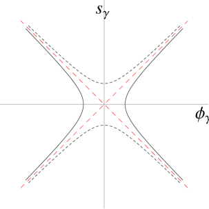
When that is in the antigravity regime, it is again possible to choose an Einstein gauge in which so the gravitational constant is negative. This amounts to switching and in Eq.(2), and consequently changing the signs of the first two terms (but not the other signs!) in the gauge fixed action in Eq.(3). Thus the Weyl invariant action in Eq.(1) includes an antigravity sector in the traditional language of the Einstein frame. The two sectors are related by simply extending the domain of the fields to cover the entire plane in Fig.1, rather than only the gravity regime defined by the restriction The question was: are the gravity/antigravity sectors connected by dynamics?
Informal conversations over two years with numerous cosmologists around the world did not produce an answer to the question of whether the dynamics compels to change sign. So an analytic study of the dynamical equations needed to be undertaken, as we did in 2010 inflation-BC . Playing with various gauge choices of the Weyl symmetry, produced tricks and methods to solve the cosmological equations analytically for some choices of the potential energy described by the function or Through the analytic solutions, it became apparent that the sign of the gauge invariant quantity can change dynamically, at least as a function of time. Note that the sign of or equivalently of is a Weyl gauge invariant. We expected that it would be hard to find solutions of the equations in which the sign changed dynamically, but instead we discovered that the change of sign happens generically. To prevent the sign switch from happening one must artificially fine tune initial conditions of the fields and/or parameters in the potential energy or We also understood that, the spacetime point(s) at which the gauge invariant factor vanishes just before changing sign in any gauge, is a curvature singularity of in the Einstein gauge. Thus, in the -gauge in which has been gauge fixed to a constant, the gauge invariant vanishes exactly at the curvature singularity, while goes to infinity to maintain the constant gauge.
Thus the sign change is a generic consequence of dynamics, and the sign can change only at a geometrical singularity. If the theory of Eq.(1) is restricted by hand to the sector then the spacetime will be cutoff at the singularity, and the theory will be geodesically incomplete. This explained precisely how the traditional formulation of gravity in the form of Eq.(3) is geodesically incomplete, since it amounts to only the geodesically incomplete positive domain . The cure to make it geodesically complete is evident: extend the Einstein frame with the Weyl symmetry (i.e. reintroduce the gauge degrees of freedom rather than just ) and add the missing antigravity domain shown in Fig.1. This extension of the domain in field space is reminiscent of the Kruskal-Szekeres extension of the domain of the spacetime metric across the horizon of the blackhole to include the interior region.
Since singularities were involved with the switching of signs, a collaboration with cosmologists ensued BCT1 -BCST2 to try to understand more thoroughly the cosmological significance of the switch of the sign of . The fact that the action in Eq.(1) could be directly related to the colliding branes scenario of a cyclic universe cyclic1 branesMT 333This is seen after massaging some more the equations in branesMT . This unpublished manipulation of the equations that made the connection more evident was developed in the process of the collaboration in BCT1 . made it even more attractive to study the model in Eq.(1) for cosmological applications.
The analytic solutions were obtained easily in another gauge called the -gauge in which the fields are labelled with the letter such as to indicate they are gauge fixed differently than some other useful gauges. The -gauge is defined by demanding that the determinant of the metric is fixed to such as
| (4) |
for all spacetime We define the following Weyl gauge invariant quantity which plays an important role in our discussion
| (5) |
Other useful gauge invariants are the ratio and the products and . By gauge invariance we can equate the gauge fixed forms of in the -gauge and in the -gauge, which yields (for all signs of )
| (6) |
This shows that when vanishes in the -gauge, the gauge invariant quantity will vanish in all gauges, while only in the -gauge the determinant of the metric will also vanish. This shows that the complete failure of the geometry in the Einstein gauge (which is when the cosmological singularity occurs, and geodesics are incomplete) is related directly to the vanishing of the factor that appears in the Weyl invariant action.
Note that the failure of the geometry in the Einstein gauge does not imply the failure of the geometry in other Weyl gauges. Recall that curvature does transform under Weyl transformations. In particular, by construction, since in all spacetime patches in the -gauge, we may expect smoother behavior of curvature components in the -gauge (even if singular for some components), as compared to more singular curvature components in the Einstein gauge . This smoother feature of the -gauge, and some additional properties of some potential energy functions or turned out to be the key factors both to geodesically complete the geometry of the Einstein frame, and to find analytically the complete set of solutions of all the fields, in a homogeneous cosmological state (i.e. purely time dependent fields).
For the purpose of cosmological studies, we concentrate on the relevant geometries of interest that can be written in the form where is the conformal time, is the scale factor of the universe, is the lapse function that plays the role of a gauge field that insures -reparameterization symmetry, and is the spacial metric in 3-dimensions in which we will include a curvature parameter and anisotropy degrees of freedom as functions of time We consider the spaces known as FRLW, Kasner, Bianchi IX and Bianchi VIII. All of these are captured by the following parametrization of the 3-dimensional part of the metric (the used in this paper are redefined as compared to BCST1 BCST2 by rescaling them with the factor so that here they are dimensionless)
| (7) |
For FRLW that has no anisotropy we set and For Kasner that has no curvature we set and for the Bianchi metrics that have both anisotropy and curvature include the curvature parameter along with dependence.
Then concentrating on purely time dependent homogeneous fields, the effective action relevant for cosmological investigations that follows from Eq.(1) is
| (8) |
where is the radiation density when the scale factor . Here is the anisotropy potential which emerges from the curvature term
| (9) |
In the isotropic limit the anisotropy potential reduces to a constant For the Kasner metric the potential energy term is absent even if anisotropy is present since
The homogeneous degrees of freedom in are the scalar fields and the geometric fields that are part of the metric. This effective action is invariant under the gauge symmetries of -reparameterization and -dependent Weyl transformations
| (10) |
while and are Weyl invariant. After using the equations of motion for (that results in the zero energy constraint), we choose the gauge Furthermore, one of the fields may be eliminated by a Weyl gauge choice; for each choice the fields are labelled with an extra index to indicate that they are the gauge fixed versions of the fields. We have discussed several gauge choices (for a subset see BCST2 ), including the Einstein gauge of Eq.(2) labelled by as the -gauge of Eq.(4) labeled by as in which , the constant (or supergravity) gauge 2Tgravity labelled by in which constant, and the string gauge labelled by BCST2 in which the action in Eq.(1) reduces to the form of the low energy effective action of string theory including the dilaton in the string frame. The -gauge is useful to discuss the physics in the Einstein frame where most of the physical intuition on gravitational physics has been developed historically. However, the cosmological field equations are non-linear and difficult to solve in the -gauge. On the other hand, in the -gauge the field equations simplify greatly to the point where they can be solved analytically to yield the full set of solutions for some cases of the potential energy or This was exploited in inflation-BC -BCST2 to obtain the results summarized in this paper.
The -gauge and -gauge degrees of freedom are related by a gauge transformation as in Eqs.(2,6) and
| (11) |
This was used to obtain the solutions for and in the Einstein frame from the solutions for in the -gauge. Similarly transformations among other gauges leads to the solutions in other gauges.
The methodical study in inflation-BC -BCST2 using analytic tools will not be repeated here. Instead, only some results will be outlined briefly. The complete set of solutions of the cosmological equations were obtained with no restrictions on either the parameters of the model or the initial conditions on the fields. Before the important role of anisotropy is taken into account near the singularity at , there are 6 unrestricted parameters in our solutions. All 6 parameters are available to try to fit cosmological data far away from the singularity. In the absence of anisotropy, the solution for behaves in various detailed ways in different regions of the 6 parameter space. This is given in the Appendix of BCST2 , where 25 different regions of the 6 parameter space are identified in which the analytic expression is different for each case separately. The trajectory of the solution in the absence of anisotropy can be plotted parametrically (by eliminating the parameter) in the plane of Fig.1. This shows that the generic trajectory crosses the lightcone in Fig.1 at any point so that keeps changing sign as the universe moves between gravity/antigravity patches. To do so, the scale factor vanishes at each crossing (according to Eq.(11)), so that the gravity/antigravity patches are connected to each other only through the cosmological singularity in the Einstein frame. It should be emphasized that the cosmological singularity in the -gauge at is not a singularity of the determinant of the -gauge metric, since . The singularity of the -gauge, which comes from the vanishing of the gauge invariant becomes in the -gauge. However, within the -gauge, in the absence of anisotropy, this is not at all singularity of the equations, and in the presence of anisotropy it is avoidable by several symmetry arguments and a complex continuation BCST1 ; this is why it was possible to integrate the equations unambiguously as and understand the geodesic completeness of the cosmological system.
An example of the generic solution in the absence of anisotropy is plotted in Fig.2a. At each crossing of the dotted diagonal lines, when at times the universe has a zero-size bounce, where it transits generically between gravity/antigravity regions. Although the analytic solutions were obtained for specific potentials, it became evident that this general behavior is generic and basically model independent.
The behavior of the generic solution near the singularity changes dramatically in the presence of anisotropy by an attractor mechanism. An important effect of anisotropy is to focus the trajectory of the generic solution to pass through the origin of the plane, such that the generic trajectory can cross the lightcone in Fig.2b only at the origin where vanish simultaneously.
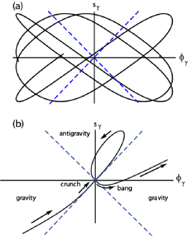
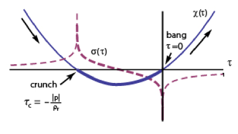
The attractor mechanism discovered in BCST1 is model independent because the potential energy or is negligible close to the singularity. It is well known that the dominant terms in the Friedmann equations in the Einstein frame are the kinetic energies for the scalar field and for anisotropy. The next to the leading term is radiation represented by the parameter in the action above. The potential energies for the scalar field and anisotropy, which appear in the action in the form are negligible as compared to the dominant terms, since, near the singularity, in the -gauge, or in the -gauge. Through our analytic analysis, we found that the mixmaster behavior described in Misner is avoided when the kinetic energy of the scalar field is a few times larger than the kinetic energy of the anisotropy fields as defined in the action of Eq.(1); this is consistent with the discussion in BKL Damour . Hence the attractor solution given analytically in BCST1 is unique and unambiguous as justified in BCST1 . Its properties are illustrated in the plots in Fig.2b and Fig.3.
In Fig.3 the plots are for the gauge invariants and Recall from Eqs.(5,11) that Hence the crunch/bang occur when and it is seen from Fig.2a that the universe goes smoothly through these singularities while undergoing transitions between the gravity and antigravity regimes. It should be emphasized that this behavior is dictated by geometry (anisotropy), it is model independent, unavoidable and unambiguous. Note also that the duration of antigravity decreases with an increase in radiation or a decrease in the kinetic energies of the scalar fields or anisotropy.
We have asked the question whether it is possible to avoid the antigravity region? The answer is different depending on the presence or absence of anisotropy. With non-zero anisotropy, no matter how small, it is not possible to avoid the antigravity region, due to the unique solution illustrated in Fig.2b and Fig.3. Since it is unlikely that anisotropy is identically zero near the singularity, the conclusion is that, at the classical level, antigravity cannot be avoided.
Nevertheless, we may still answer the question when anisotropy is identically zero. Then the answer is yes, antigravity can be avoided, and still have a geodesically complete universe in the Einstein frame, confined only to the gravity patches in Fig.1. This is described by a non-generic subset of special solutions that are obtained by restricting the parameter space or initial conditions, and they describe zero-size and finite-size bounces, as shown in Figs.(4-7) and Figs.(8,9) respectively. As seen in Figs.(6,7), the trajectories of the zero-size bounces never reach into the antigravity sector and they never cross the dotted diagonals except at the origin.
![[Uncaptioned image]](/html/1209.1068/assets/x4.png) Fig.4 - Zero-size bounces in a cyclic universe.
and for are depicted. In this example of
an analytic solution for the case of the fields are computed through
Eq.(11), so the behavior at crunch/bang times is consistent with
Fig.5. The number corresponds to the number of times crosses
zero between a bang and a crunch, and is related to the qantization of periods
described in Fig.5. For (not shown) turnaround is at
Fig.4 - Zero-size bounces in a cyclic universe.
and for are depicted. In this example of
an analytic solution for the case of the fields are computed through
Eq.(11), so the behavior at crunch/bang times is consistent with
Fig.5. The number corresponds to the number of times crosses
zero between a bang and a crunch, and is related to the qantization of periods
described in Fig.5. For (not shown) turnaround is at
|
![[Uncaptioned image]](/html/1209.1068/assets/x5.png) Fig.5 - Zero-size bounces in a cyclic universe. and for are depicted.
In this example of an analytic solution for the case of potential energy
with , the fields
, have
synchronized initial values, and relatively quantized half periods (6 to 1 as seen
in the figure) so that vanish simultaneously at all
cyclic crunch/bang times. For (not shown) turnaround is at The same solution is potted in Figs.6,7 in a
different way.
Fig.5 - Zero-size bounces in a cyclic universe. and for are depicted.
In this example of an analytic solution for the case of potential energy
with , the fields
, have
synchronized initial values, and relatively quantized half periods (6 to 1 as seen
in the figure) so that vanish simultaneously at all
cyclic crunch/bang times. For (not shown) turnaround is at The same solution is potted in Figs.6,7 in a
different way.
|
The zero-size-bounce in Figs.(4-7) describes a cyclic universe that contracts to zero size and then bounces back smoothly from zero size. They are exact analytic solutions of the cosmological equations for the case of or equivalently The universe expands up to either a finite size (when ) or infinite size (when ) and then turns around to repeat the cycle. In these solutions, as described in detail in BCT1 BCST2 , the behavior of near the singularity at is smooth (if or take generic values, then ; if both vanish or take some special values, then Also, the behavior of the potential and kinetic energy terms for the scalar field near the singularity are surprising. Namely, contrary to the generic solution, the potential energy dominates over the kinetic energy so that the equation of state is negative near the singularity. According to common lore, it was thought that such zero-size-bounce solutions would not exist because they would violate the null energy condition (NEC). However, this is not the case. The NEC is satisfied because there is a singularity at zero size, and this is the exception allowed according to the NEC theorems. To emphasize, the singularity theorems are not violated, there is a singularity in the Einstein frame, but what was missed is that it is possible to have a bounce of zero size, as explicitly given analytically in our papers. We found all such solutions and classified them in BCT1 BCST2 , thus providing a rich class of examples of zero-size-bounce cyclic universes, characterized by arbitrary values of the parameters plus one additional quantized parameter ( in Figs.4-7).
To make the zero-size-bounce happen, a synchronization of initial conditions and a quantization condition among the 6 available parameters must be imposed. These properties are illustrated in Fig.5, where it is seen is imposed as an initial condition, and the periods of oscillations of and are quantized relative to each other. Hence such solutions are characterized by 4 continuous and 1 quantized parameter, rather than the 6 continuous parameters of the generic solutions. In that sense the zero-size-bounce solutions are a set of measure zero. So, statistically, it does not seem likely that the universe would choose such a solution over the generic solution.
However, anisotropy plays a very important role in providing an attractor mechanism such that, for typical initial conditions away from the singularity, all trajectories are attracted to the origin of the plane and can cross the lightcone in Fig.1 only at the origin. In that sense the type of solution depicted in Figs.(4-7) is not too far from being generic once anisotropy is taken into account. In particular the behavior away from the origin is a good approximation. Nevertheless, what goes on at the singularity is quite different than what is depicted in Figs.(4-7). Namely, antigravity cannot be avoided since the non-generic solutions of Figs.(4-7) become strongly distorted by anisotropy, so that near the singularity they approach the point tangentially to the dotted diagonal lines, with the same absolute rate (which is different when anosotropy is absent), and must dive into the antigravity region just as depicted in Fig.(2b,3), which is different than Figs.6,7.
In the absence of anisotropy there are also non-generic finite size solutions. The analytic solutions for these are given in BCT1 BCST2 , and an example is depicted in Figs.(8.9). These are also repetitive as a function of time, although not fully cyclic in the sense that the minimum size of the universe (and other properties) could change from cycle to cycle.
![[Uncaptioned image]](/html/1209.1068/assets/x8.png) Fig.8 - Finite-size-bounce, for all . It is possible only in a narrow range
of parameter space, including a condition on inital values in the range
Fig.8 - Finite-size-bounce, for all . It is possible only in a narrow range
of parameter space, including a condition on inital values in the range
|
![[Uncaptioned image]](/html/1209.1068/assets/x9.png) Fig.9 - Finite-size-bounce. The scale factor, never vanishes as
seen from Eq.(11) and Fig.8. The minumum size of varies from cycle to cycle.
Fig.9 - Finite-size-bounce. The scale factor, never vanishes as
seen from Eq.(11) and Fig.8. The minumum size of varies from cycle to cycle.
|
The finite-size-bounce describes a universe that contracts up to a minimum non-zero size and then bounces back into an expansion phase up to infinite size. As the universe turns around to repeat such cycles the minimum size is not necessarily the same, as this depends on the parameters and initial conditions. Such solutions occur when the parameters satisfy, and ; for details see BCST2 . Note that there are still 6 parameters, so this is not a set of measure zero, but it is a restricted small region of parameter space or initial values.
In the presence of anisotropy these solutions are also distorted. However, since never vanished when anisotropy was neglected, the effects of anisotropy may be less important. We have not fully determined if, depending on initial conditions, it may be possible to avoid the antigravity region for all values of the conformal time . Even if this is possible mathematically, since it corresponds to a very small region in the space of parameters of the model and initial conditions, it seems it is an unlikely physical scenario.
We are, therefore, faced with trying to understand physical phenomena in the antigravity regime. Some relevant ideas are found in BCST1 BCST2 . These include comments on negetive energy gravitons, an analogy to the Klein-Paradox, and an outline on analytic continuations to circumvent the singularity to connect data from before the crunch to after the bang, etc.. The difficult, but ultimately necessary, ingredient is the inclusion of the full, possibly non-perturbative, quantum effects, that remain as a challenge. However, progress and physical insight into the meaning and measurable effects of antigravity are likely to develop well before understanding the full theory of quantum gravity.
IV Conclusions and Outlook
This paper summarized our approach with analytic solutions of cosmological equations to discuss geodesic completeness through the big bang singularity. This analysis was done in the purely classical theory of gravity, but has some immediate extensions to the quantum theory. In particular, in the context of the path integral, our complete set of classical solutions provide a semi-classical approximation to the quantum theory of gravity (like instantons in QCD). Furthermore, in the context of string theory, our complete set of solutions provide cosmological backgrounds consistent with perturbative conformal invariance on the worldsheet, and hence a starting point for a stringy investigation of quantum gravity in a cosmological setting.
We learned that the generic solution shows that the trajectory of the universe goes smoothly through the crunch/bang singularities while traversing from gravity to antigravity spacetime patches, and doing this repeatedly in a periodic manner. The generic trajectory can cross the “lightcone” in field space, as shown in Fig.(2a), at any place, if anisotropy vanishes. The crossing points on the “lightcone” depend on the parameters of the model and initial conditions. When anisotropy is present, there is an attractor mechanism that distorts the generic solution close to the singularity to the form shown in Fig.2b and Fig.3. This is model independent, unique and unavoidable at the classical level. Therefore, the phenomenon of antigravity should be considered seriously in discussing cosmology.
It is possible to avoid antigravity and still have a geodesically complete geometry, but only if anisotropy vanishes identically, which is an unlikely scenario for the initial stages of a small universe, and only within a smaller subset of initial conditions, which is of measure zero in the space of all initial conditions. If these unjustifiable conditions are assumed, then the zero-size bounces of the type in Figs.(4-7) and the finite size-bounces of the type in Figs.(8,9) are the only geodesically complete solutions contained totally within the traditional Einstein frame. One group of trajectories passes through the center of the “lightcone”repeatedly, resulting in a cyclic universe as in Figs.(4-7). These solutions, which do not violate the null energy condition, provide a set of examples that bouncing at zero size is possible classically in cosmological scenarios with or without spatial curvature.
We have shown that antigravity is very hard to avoid generically in the classical theory. Anisotropy + radiation + kinetic energy of the scalar field require the antigravity epoch. For close to a year we tried to find models and mechanisms to avoid antigravity (i.e. when all solutions of a geodesically complete model are included). The failure to find such mechanisms finally led us to take antigravity seriously. We also studied the Wheeler-deWitt equation to take into account some quantum effects for the same system that we analyzed classically. We could solve some cases exactly, others semi-classically. We arrived substantially to the same conclusions that we learned by studying the purely classical system.
The source of antigravity is the factor that can switch sign and becomes negative in the antigravity regimes indicted in Fig.1. This factor is a consequence of the Weyl symmetry as explained following Eq.(1). It cannot be replaced by the absolute value to avoid the sign change because this is not Weyl invariant. There are generalizations of this factor consistent with Weyl symmetry as given in footnote (1) and 2tSugra , but after taking into account additional features, such as supersymmetry, there are no variations of this factor that would not switch sign. Note from Eqs.(2,11) that the signature of the metric does not change when when this factor switches sign. In 1T-physics Weyl symmetry is not required, so gravity can be formulated without the antigravity sector, but as described following Fig.1, such a formulation of gravity is necessarily geodesically incomplete, and therefore problematic. By contrast, in 2T-physics Weyl symmetry is a consequence of just the presence of the extra dimensions since Weyl symmetry amounts to a reparametrization of the coordinates as part of the general coordinate invariance in dimensions (note that Weyl symmetry is not a symmetry of 2T-gravity 2Tgravity 2TgravityGeometry on top of general coordinate invariance in ). So, Weyl symmetry may be considered a feature and signature of 2T-physics.
It should be emphasized that our new results transcend the specific simple models for which we found the complete set of analytic solutions. The phenomena we have found should also be expected generically in supergravity theories coupled to matter whose formulation include a similar factor that multiplies In supergravity, that factor has the form where the function of the compex fields is called the Kähler potential. In the past, it was assumed that the overall factor in front of is positive, and investigations of supergravity proceeded, by fiat, only in the positive regime weinberg . For example, a discussion of the field space in the positive sector for general =2 supergravity can be found in deWit . However, our results suggest that generically the overall factor can and will change sign dynamically, in every gauge, and therefore in the geodesically complete supergravity, antigravity sectors similar to our discussion in this paper should be expected in typical supergravity theories (this is illustrated with an example in BCST3 ).
As emphasized above, in supergravity, the factor in front of is not generally positive definite. To clarify this point in the context of our formalism, we could chose a gauge in our simple theory to make it look like supergravity. In a Weyl gauge that we call the supergravity gauge, or -gauge 2Tgravity BCST2 , in which is set to a constant , our gauge fixed term reduces precisely to the familiar form in supergravity, including a Kähler potential. As we have argued, if changes sign in one gauge, it must change sign in every gauge, because the sign is gauge invariant under Weyl transformations. Hence, the similar factor in supergravity is also expected to change sign. This can be made more evident in a Weyl invariant reformulation of supergravity. This is not straightforward because scalar fields in supergravity are complex, so a complex would have an additional ghost that needs removal with a larger gauge symmetry beyond the Weyl symmetry. I have shown in 2tSugra that the general Weyl invariant approach can in fact be extended to supergravity where an additional U gauge symmetry exists to remove the ghosts of a complex field. Similarly, in supergravities with more supersymmetries there are additional hidden gauge symmetries that enlarge the hidden gauge group, which, together with the Weyl symmetry can remove ghosts like ; this allows the inclusion of more fields like that further generalize the factor analogous to and thus permitting a richer variety of useful gauge choices. So, the form that occurs in supergravity is just the -gauge fixed version of the supersymmetric Weyl invariant supergravity formalism; this was derived again from a dimensional 2T-supergravity 2tSugra . There is however one additional constraint placed on as a result of the underlying dimensional structure of 2T-supergravity: this constraint on scalar fields, as given in 2tSugra , which applies in all fundamental theories of physics, including the Higgs field in the Standard model, may be taken as another feature and signature of 2T-physics which may show up in cosmology and/or accelerator physics.
Until better understood in the context of quantum gravity, or string theory, our results should be considered to be a first pass for the types of new physics questions they raise and the answers they provide. Much remains to be understood, including quantum gravity and string theory effects, but it is clear that previously unsuspected phenomena, including antigravity, come into play classically close to the cosmological singularity. The technical tools to study such issues in the context of a full quantum theory of gravity are yet to be developed. This is an important challenge, since the results have profound implications for both fundamental physics and our understanding of the origin, evolution and future of the universe.
Acknowledgements.
This research was partially supported by the U.S. Department of Energy under grant number DE-FG03-84ER40168. I would like to thank my collaborators Shih-Hung Chen, Paul Steinhardt and Neil Turok with whom this research was conducted.References
- (1) S. Hawking and G.F.R. Ellis, The Large Scale Structure of Space Time, Cambridge University Press (1973), ISBN 0-521-09906-4.
- (2) S. Hawking and R. Penrose. The Nature of Space and Time, Princeton University Press (1996), ISBN 0-691-03791-4; S.W. Hawking, “The Nature of Space and Time”, arXiv:hep-th/9409195v1.
- (3) I. Bars and S-H. Chen, “The Big Bang and Inflation United by an Analytic Solution”, Phys. Rev. D83 (2011) 043522 [arXiv:1004.0752].
- (4) I. Bars, S-H. Chen and N. Turok, “Geodesically Complete Analytic Solutions for a Cyclic Universe”, Phys. Rev. D 84 083513 (2011) [arXiv:1105.3606 [hep-th]].
- (5) I. Bars, “Geodesically Complete Universe”, arXiv:1109.5872 [gr-qc], in the Proceedings of the DPF-2011 Conference, Providence, RI, (2011).
- (6) I. Bars, S-H. Chen, P. Steinhardt and N. Turok, “Antigravity and the Big Crunch/Big Bang Transition”, Phys.Lett. B715 (2012) 278 [ arXiv:1112.2470 [hep-th]].
- (7) I. Bars, S-H. Chen, P. Steinhardt and N. Turok, “Complete Set of Homogeneous Isotropic Analytic Solutions in Scalar-Tensor Cosmology with Radiation and Curvature”, arXiv:1207.1940 [hep-th], submitted to Phys. Rev.
- (8) I. Bars, P. Steinhardt and N. Turok, “Cosmological History of the Higgs Field”, in preparation.
- (9) A. H. Guth, Phys. Rev. D23, 347 (1981).
- (10) A. D. Linde, Phys. Lett. B108, 389 (1982).
- (11) A. Albrecht, P. J. Steinhardt, Phys. Rev. Lett. 48, 1220 (1982).
- (12) For discussions, see P. J. Steinhardt, Sci. Am. 304, 36-43 (2011) and N. Turok, http://pirsa.org/11070044.
- (13) P. J. Steinhardt and N. Turok, Science 296, 1436 (2002).
- (14) J. Khoury, B. A. Ovrut, P. J. Steinhardt and N. Turok, Phys. Rev. D64, 123522 (2001) [arXiv:hep-th/0103239].
- (15) J. K. Erickson, D. H. Wesley, P. J. Steinhardt and N. Turok, Phys. Rev. D69, 063514 (2004) [arXiv:hep-th/0312009].
- (16) E. Buchbinder, J. Khoury, and B. A. Ovrut, Phys. Rev. D76, 123503 (2007).
- (17) L. Anderson and A. D. Rendall, Comm. Math. Phys., 218, 479 (2001).
- (18) I. Bars, “Gauge Symmetry in Phase Space, Consequences for Physics and Spacetime”, Int. J. Mod. Phys. A25 (2010) 5235 [arXiv:1004.0688 [hep-th]].
- (19) I. Bars and J. Terning, Extra Dimensions in Space and Time, Springer, NY (2010), ISBN 978-0-387-77637-8.
- (20) H. Weyl, “Spacetime Matter” (Dover, NY, 1922), sect.35; Sitzungsber. Preuss Acad. d. Wissensch (1918) 465, reprinted in The Principles of Relativity (Dover, NY, 1923).
- (21) I. Bars, ”Gravity in 2T-Physics”, Phys. Rev. D77 (2008) 125027 [arXiv:0804.1585[hep-th]].
- (22) I. Bars, S. H. Chen ”Geometry and Symmetry Structures in 2T Gravity”, Phys. Rev. D79 (2009) 085021 [arXiv:0811.2510 [hep-th]].
- (23) S. Deser, Annals of Phys. 59 (1970) 248.
- (24) I. Bars, “The Standard Model of Particles and Forces in the Framework of 2T-physics,” Phys. Rev. D74 (2006) 085019 [hep-th/0606045].
- (25) I. Bars, “The Standard model as a 2T-physics theory,” hep-th/0610187 or AIP Conf.Proc. 903 (2007) 550 (DOI: 10.1063/1.2735245).
- (26) I. Bars, “Constraints on Interacting Scalars in 2T Field Theory and No Scale Models in 1T Field Theory”, Phys. Rev. D82 (2010) 125025 [arXiv:1008.1540].
- (27) P. McFadden, P. J. Steinhardt and N. Turok, Phys. Rev. D76, 104038 (2007). P. McFadden and N. Turok, “Conformal Symmetry of Brane World Effective Actions”, Phys. Rev. D71 (2005) 021901 [arXiv:hep-th/0409122].
- (28) C. W. Misner, Phys. Rev. Lett. 22 (1969) 1071.
- (29) V. A. Belinsky, I. M. Khalatnikov, E. M. Lifshitz, Adv. Phys. 19 525 (1970).
- (30) T. Damour, M. Henneaux, H. Nicolai, “Cosmological Billiards”, Class. Quant. Grav. 20 R145 (2003)
- (31) See for example Eq.(31.6.62) in S. Weinberg, The Quantum Theory of Fields, Volume III, Cambridge 2000.
- (32) B. de Wit and A. Van Proeyen, “Potentials and Symmetries of General Gauged =2 Supergravity: Yang-Mills Models”, Nucl.Phys. B245 (1984) 89.