Efficient EM Training of Gaussian Mixtures with Missing Data

Abstract

In data-mining applications, we are frequently faced with a large fraction of missing entries in the data matrix, which is problematic for most discriminant machine learning algorithms. A solution that we explore in this paper is the use of a generative model (a mixture of Gaussians) to compute the conditional expectation of the missing variables given the observed variables. Since training a Gaussian mixture with many different patterns of missing values can be computationally very expensive, we introduce a spanning-tree based algorithm that significantly speeds up training in these conditions. We also observe that good results can be obtained by using the generative model to fill-in the missing values for a separate discriminant learning algorithm.

I Introduction

The presence of missing values in a dataset often makes it difficult to apply a large class of machine learning algorithms. In many real-world data-mining problems, databases may contain missing values due directly to the way the data is obtained (e.g. survey or climate data), or also frequently because the gathering process changes over time (e.g. addition of new variables or merging with other databases). One of the simplest ways to deal with missing data is to discard samples and/or variables that contain missing values. However, such a technique is not suited to datasets with many missing values; these are the focus of this paper.

Here, we propose to use a generative model (a mixture of Gaussians with full covariances) to learn the underlying data distribution and replace missing values by their conditional expectation given the observed variables. A mixture of Gaussians is particularly well suited to generic data-mining problems because:

• By varying the number of mixture components, one can combine the advantages of simple multivariate parametric models (e.g. a single Gaussian), that usually provide good generalization and stability properties, to those of non-parametric density estimators (e.g. Parzen windows, that puts one Gaussian per training sample [2]), that avoid making strong assumptions on the underlying data distribution.

• The Expectation-Maximization (EM) training algorithm [3] naturally handles missing values and provides the missing values imputation mechanism. One should keep in mind that the EM algorithm assumes the missing data are “Missing At Random” (MAR), i.e. that the probability of variables to be missing does not depend on the actual value of missing variables. Even though this assumption will not always hold in practical applications like those mentioned above, we note that applying the EM algorithm might still yield sensible results in the absence of theoretical justifications.

• Training a mixture of Gaussians scales only linearly with the number of samples, which is attractive for large datasets (at least in low dimension, and we will see in this paper how large-dimensional problems can be tackled).

• Computations with Gaussians often lead to analytical solutions that avoid the use of approximate or sampling methods.

• When confronted with the supervised problem of learning a function $y=f(x)$, a mixture of Gaussians trained to learn a joint density $p(x,y)$ directly provides a least-square estimate of $f(x)$ by $\hat{y}=E[Y|x]$.

Even though such mixtures of Gaussians can indeed be applied directly to supervised problems [4], we will see in experiments that using them for missing value imputation before applying a discriminant learning algorithm yields better results. This observation is in line with the common belief that generative models that are trained to learn the global data distribution are not directly competitive with discriminant algorithms for prediction tasks [5]. However, they can provide useful information regarding the data that will help such discriminant algorithms to reach better accuracy.

The contributions in this paper are two-fold:

1. We explain why the basic EM training algorithm is not practical in large-dimensional applications in the presence of missing values, and we propose a novel training algorithm that significantly speeds it up.

2. We show, both by visual inspection on image data and by for imputed values for classification, how a mixture of Gaussians can model the data distribution so as to provide a valuable tool for missing values imputation.

Note that an extensive study of Gaussian mixture training and missing value imputation algorithms is out of the scope of this paper. Various variants of EM have been proposed in the past (e.g. [6]), while we focus here on the “original” EM, showing how it can be solved exactly at a significantly lower computational cost. For missing value imputation, statisticians may prefer to draw from the conditional distribution instead of inputing its mean, as the former better preserves data covariance [7]. In machine learning, the fact that a value is missing may also be by itself a useful piece of information worth taking into account (for instance by adding extra binary inputs to the model, indicating whether each value was observed). All these are important considerations that one should keep in mind, but they will not be addressed here.

II EM for Gaussian Mixtures with Missing Data

In this section, we present the EM algorithm for learning a mixture of Gaussians on a dataset with missing values. The notations we use are as follows. The training set is denoted by ${\cal D}=\{x^{1},\ldots,x^{n}\}$. Each sample $x^{i}\in\mathbbm{R}^{d}$ may have different missing variables. A missing pattern is a maximal set of variables that are simultaneously missing in at least one training sample. When the input dimension $d$ is high, there may be many different missing patterns, possibly on the same order as the number of samples $n$ (since the number of possible missing patterns is $2^{d}$). For a sample $x^{i}$, we denote by $x^{i}_{o}$ and $x^{i}_{m}$ the vectors corresponding to respectively the observed and missing variables in $x^{i}$. Similarly, given $x^{i}$, a symmetric $(d\times d)$ matrix $M$ can be split into four parts corresponding to the observed and missing variables in $x^{i}$, as follows:

• $M_{oo}$ contains elements $M_{kl}$ where variables $k$ and $l$ are observed in $x^{i}$,

• $M_{mm}$ contains elements $M_{kl}$ where both variables $k$ and $l$ are missing in $x^{i}$,

• $M_{om}=M_{mo}^{T}$ contains elements $M_{kl}$ where variable $k$ is observed in $x^{i}$, while variable $l$ is missing.

It is important to keep in mind that with these notations, we have for instance $M_{mm}^{-1}\overset{\underset{\mathrm{def}}{}}{=}(M_{mm})^{-1}\neq(M^{-1})_{mm}$, i.e. the inverse of a sub-matrix is not the sub-matrix of the inverse. Also, although to keep notations simple we always write for instance $M_{oo}$, the observed part depends on the sample currently being considered: for two different samples, the $M_{oo}$ matrix may represent a different sub-part of $M$. It should be clear from the context which sample is being considered.

The EM algorithm [3] can be directly applied in the presence of missing values [8]. As shown in [4], for a mixture of Gaussians the computations for the two steps (Expectation and Maximization) of the algorithm are:

Expectation

compute $p_{ij}$, the probability that Gaussian $j$ generated sample $x^{i}$. For the sake of clarity in notations, let us denote $\mu=\mu_{j}^{(t)}$ and $\Sigma=\Sigma_{j}^{(t)}$ the estimated mean and covariance of Gaussian $j$ at iteration $t$ of the algorithm. To obtain $p_{ij}$ for a given sample $x^{i}$ and Gaussian $j$, we first compute the density

$$q_{ij}={\cal N}(x^{i}_{o};\mu_{o},\Sigma_{oo})$$ (1)

where ${\cal N}(\cdot;\mu_{o},\Sigma_{oo})$ is the Gaussian distribution of mean $\mu_{o}$ and covariance $\Sigma_{oo}$:

$${\cal N}(z;\mu_{o},\Sigma_{oo})=\frac{1}{\sqrt{2\pi|\Sigma_{oo}|^{d}}}e^{(-\frac{1}{2}(z-\mu_{o})^{T}\Sigma^{-1}_{oo}(z-\mu_{o}))}.$$ (2)

$p_{ij}$ is now simply given by

$$p_{ij}=\frac{q_{ij}}{\sum_{\ell=1}^{L}q_{i\ell}}$$

where $L$ is the total number of Gaussians in the mixture.

Maximization

first fill-in missing values, i.e. define, for each Gaussian $j$, $\hat{x}^{i,j}$ by $\hat{x}^{i,j}_{o}=x^{i}_{o}$ and $\hat{x}^{i,j}_{m}$ being equal to the expectation of the missing values $x^{i}_{m}$ given the observed $x^{i}_{o}$, assuming Gaussian $j$ has generated $x^{i}$. Denoting again $\mu=\mu_{j}^{(t)}$ and $\Sigma=\Sigma_{j}^{(t)}$, this expectation is equal to

$$\hat{x}^{i,j}_{m}=\mu_{m}+\Sigma_{mo}\Sigma_{oo}^{-1}(x^{i}_{o}-\mu_{o}).$$ (3)

From these $\hat{x}^{i,j}$, the Maximization step of EM yields the new estimates for the mean and covariances of the Gaussians:

$$\mu_{j}^{(t+1)}=\frac{\sum_{i=1}^{n}p_{ij}\hat{x}^{i,j}}{\sum_{i=1}^{n}p_{ij}}$$

$$\Sigma_{j}^{(t+1)}=\frac{\sum_{i=1}^{n}p_{ij}(\hat{x}^{i,j}-\mu_{j}^{(t+1)})(\hat{x}^{i,j}-\mu_{j}^{(t+1)})^{T}}{\sum_{i=1}^{n}p_{ij}}+C_{j}^{(t)}.$$

The additional term $C_{j}^{(t)}$ results from the imputation of missing values by their conditional expectation, and is computed as follows (for the sake of clarity, we denote $C_{j}^{(t)}$ by $C$ and $\Sigma_{j}^{(t)}$ by $\Sigma$):

1. $C$ $\leftarrow$ 0

2. for each $x^{i}$ with observed and missing parts $x^{i}_{o}$, $x^{i}_{m}$:

   $$C_{mm}\leftarrow C_{mm}+\frac{p_{ij}}{\sum_{k=1}^{n}p_{kj}}\left(\Sigma_{mm}-\Sigma_{mo}\Sigma_{oo}^{-1}\Sigma_{om}\right)$$ (4)

The term being added for each sample corresponds to the covariance of the missing values $x^{i}_{m}$.

Regularization can be added into this framework for instance by adding a small value to the diagonal of the covariance matrix $\Sigma_{j}^{(t)}$, or by keeping only the first $k$ principal components of this covariance matrix (filling the rest of the data space with a constant regularization coefficient).

III Scaling EM to Large Datasets

While the EM algorithm naturally extends to problems with missing values, doing so comes with a high computational cost. As we will show, the computational burden may be mitigated somewhat by exploiting the similarity between the covariance matrices between “nearby” patterns of missing values. Before we delve into the details of our algorithm, let us first analyze the computational costs of the EM algorithm presented above, for each individual training sample $x^{i}$:

• The evaluation of $q_{ij}$ from eq. 1 and 2 requires the inversion of $\Sigma_{oo}$, which costs $O(n_{o}^{3})$ operations, where $n_{o}$ is the number of observed variables in $x^{i}$.

• The contribution to $C_{j}^{(t)}$ for each Gaussian $j$ (eq. 4) can be done in $O(n_{o}^{2}n_{m}+n_{o}n_{m}^{2})$ (computation of $\Sigma_{mo}\Sigma_{oo}^{-1}\Sigma_{om}$), or in $O(n_{m}^{3})$ if $\Sigma^{-1}$ is available, because:

  $$\Sigma_{mm}-\Sigma_{mo}\Sigma_{oo}^{-1}\Sigma_{om}=(\Sigma^{-1})_{mm}^{-1}.$$ (5)

Note that for two examples $x^{i}$ and $x^{k}$ with exactly the same pattern of missing variables, the two expensive operations above need only be performed once, as they are the same for both $x^{i}$ and $x^{k}$. But in high-dimensional datasets without a clear structure in the missing values, most missing patterns are not shared by many samples. For instance, in a real-world financial dataset we have been working on, the number of missing patterns is about half the total number of samples. Since each iteration of EM has a cost of $O(pLd^{3})$, with $p$ unique missing patterns, $L$ components in the mixture, and input dimension $d$, the EM algorithm as presented in section II is not computationally feasible for large high-dimensional datasets. The “fast” EM variant proposed in [6] also suffers from the same bottlenecks, i.e. it is fast only when there are few unique missing patterns.

While the large numbers of unique patterns of missing values typically found in real-world datasets present a barrier to the application of EM to these problems, they also motivate a means of reducing the computational cost. As discussed above, for high-dimensional datasets, the computational cost is dominated by the determination of the inverse covariance of the observed variables $\Sigma_{oo}^{-1}$ and of the conditional covariance of the missing data given the observed data (eq. 5). However, as we will show, these quantities corresponding to one pattern of the missing values may be determined from those of another pattern of missing values at a cost proportional to the distance between the two missing value patterns (measured as the number of missing and observed variables on which the patterns differ). Thus, for “nearby” patterns of missing values, these covariance computations may be efficiently computed by chaining their computation through the set of patterns of missing values. Furthermore, since the cost of these updates will be smaller when the missing patterns of two consecutive samples are close to each other, we want to optimize the samples ordering so as to minimize this cost.

We present the details of the proposed algorithms in the following sections. First, we observe in section III-A how we can avoid computing $\Sigma_{oo}^{-1}$ by using the Cholesky decomposition of $\Sigma_{oo}$. Then we show in section III-B how the so-called inverse variance lemma can be used to update the conditional covariance matrix (eq. 5) for a missing pattern given the one computed for another missing pattern. As presented in section III-C, these two ideas combined give rise to an objective function with which one can determine an optimal ordering of the missing patterns, minimizing the overall computational cost. The resulting fast EM algorithm is summarized in section III-D.

III-A Cholesky Updates

Computing $q_{ij}$ by eq. 1 can be done directly from the inverse covariance matrix $\Sigma_{oo}^{-1}$ as in eq. 2, but, as argued in [9], it is just as fast, and numerically more stable, to use the Cholesky decomposition of $\Sigma_{oo}$. Writing $\Sigma_{oo}=LL^{T}$ with $L$ a lower triangular matrix with positive diagonal elements, we indeed have

$$z^{T}\Sigma^{-1}_{oo}z=\|L^{-1}z\|^{2}$$

where $L^{-1}z$ can easily be obtained since $L$ is lower triangular. Assuming $L$ is computed once for the missing pattern of the first sample in the training set, the question is thus how to update this matrix for the next missing pattern. This reduces to finding how to update $L$ when adding or removing rows and columns to $\Sigma_{oo}$ (adding a row and column when a variable that was missing is now observed in the next sample, and removing a row and column when a variable that was observed is now missing).

Algorithms to perform these updates can be found for instance in [10]. When adding a row and column, we always add it as the last dimension to minimize the computations. These are on the order of $O(n_{o}^{2})$, where $n_{o}$ is the length and width of $\Sigma_{oo}$. Removing a row and column is also on the order of $O(n_{o}^{2})$, though the exact cost depends on the position of the row / column being removed.

Let us denote by $n_{d}$ the number of differences between two consecutive missing patterns. Assuming that $n_{d}$ is small compared to $n_{o}$, the above analysis shows that the overall cost is on the order of $O(n_{d}\;n_{o}^{2})$ computations. How to find an ordering of the patterns such that $n_{d}$ is small will be discussed in section III-C.

III-B Inverse Variance Lemma

The second bottleneck of the EM algorithm resides in the computation of eq. 5, corresponding to the conditional covariance of the missing part given the observed part. Note that we cannot rely on a Cholesky decomposition here, since we need the full conditional covariance matrix itself. In order to update $(\Sigma^{-1})_{mm}^{-1}$, we will take advantage of the so-called inverse variance lemma [11]. It states that the inverse of a partitioned covariance matrix

$$\Lambda=\left(\begin{array}[]{cc}\Lambda_{XX}&\Lambda_{XY}\\ \Lambda_{YX}&\Lambda_{YY}\end{array}\right)$$ (6)

can be computed by

$$\Lambda^{-1}=\left(\begin{array}[]{cc}\Lambda_{XX}^{-1}+B^{T}\Lambda_{Y|X}^{-1}B&-B^{T}\Lambda_{Y|X}^{-1}\\ -\Lambda_{Y|X}^{-1}B&\Lambda_{Y|X}^{-1}\end{array}\right)$$ (9)

where $\Lambda_{XX}$ is the covariance of the $X$ part, and the matrix $B$ and the conditional covariance $\Lambda_{Y|X}$ of the $Y$ part given $X$ are obtained by

$$B=\Lambda_{YX}\Lambda_{XX}^{-1}$$ (10)

$$\Lambda_{Y|X}=\Lambda_{YY}-\Lambda_{YX}\Lambda_{XX}^{-1}\Lambda_{XY}$$ (11)

Note that eq. 11 is similar to eq. 5, since the conditional covariance of $Y$ given $X$ verifies

$$\Lambda_{Y|X}=(\Lambda^{-1})_{YY}^{-1}$$ (12)

where we have also partitioned the inverse covariance matrix as

$$\Lambda^{-1}=\left(\begin{array}[]{cc}(\Lambda^{-1})_{XX}&(\Lambda^{-1})_{XY}\\ (\Lambda^{-1})_{YX}&(\Lambda^{-1})_{YY}\end{array}\right).$$ (13)

These equations can be used to update the conditional covariance matrix of the missing variables given the observed variables when going from one missing pattern to the next one, so that it does not need to be re-computed from scratch. Let us first consider the case of going from sample $x^{i}$ to $x^{j}$, where we only add missing values (i.e. all variables that are missing in $x^{i}$ are also missing in $x^{j}$). We can apply the inverse variance lemma (eq. 9) with the following quantities:

• $\Lambda^{-1}$ is the conditional covariance of the missing variables in $x^{j}$ given the observed variables, i.e. $(\Sigma^{-1})_{mm}^{-1}$ in eq. 5, the quantity we want to compute,

• $X$ are the missing variables in sample $x^{i}$,

• $Y$ are the missing variables in sample $x^{j}$ that were not missing in $x^{i}$,

• $\Lambda_{XX}^{-1}$ is the conditional covariance of the missing variables in $x^{i}$ given the observed variables, that would have been computed previously,

• since $\Lambda=(\Sigma^{-1})_{mm}$, then $\Lambda_{YX}$ and $\Lambda_{YY}$ are simply sub-matrices of the global inverse covariance matrix, that only needs to be computed once (per iteration of EM).

Let us denote by $n_{d}$ the number of missing values added when going from $x^{i}$ to $x^{j}$, and by $n_{m}$ the number of missing values in $x^{i}$. Assuming $n_{d}$ is small compared to $n_{m}$, then the computational cost of eq. 9 is dominated by the cost $O(n_{d}\;n_{m}^{2})$ for the computation of $B$ by eq. 10 and of the upper-left term in eq. 9 (the inversion of $\Lambda_{Y|X}$ is only in $O(n_{d}^{3})$).

In the case where we remove missing values instead of adding some, this corresponds to computing $\Lambda_{XX}^{-1}$ from $\Lambda^{-1}$ using eq. 9. This can be done from the partition of $\Lambda^{-1}$ since, by identifying eq. 9 and 13, we have:

$$(\Lambda^{-1})_{XX}-(\Lambda^{-1})_{XY}(\Lambda^{-1})_{YY}^{-1}(\Lambda^{-1})_{YX}$$

$$= \Lambda_{XX}^{-1}+B^{T}\Lambda_{Y|X}^{-1}B-B^{T}\Lambda_{Y|X}^{-1}(\Lambda^{-1})_{YY}^{-1}\Lambda_{Y|X}^{-1}B$$

$$= \Lambda_{XX}^{-1}$$

where we have used eq. 12 to obtain the final result. Once again the cost of this computation is dominated by a term of the form $O(n_{d}\;n_{m}^{2})$, where this time $n_{d}$ denotes the number of missing values that are removed when going from $x^{i}$ to $x^{j}$ and $n_{m}$ the number of missing values in $x^{j}$.

Thus, in the general case where we both remove and add missing values, the cost of the update is on the order of $O(n_{d}\;n_{m}^{2})$, if we denote by $n_{d}$ the total number of differences in the missing patterns, and by $n_{m}$ the average number of missing values in $x^{i}$ and $x^{j}$ (which are assumed to be close, since $n_{d}$ is supposed to be small). The speed-up is on the order of $O(n_{m}/n_{d})$ compared to the “naive” algorithm that would re-compute the conditional covariance matrix for each missing pattern.

III-C Optimal Ordering From the Minimum Spanning Tree

Given an ordering $\{m^{1},m^{2},\ldots,m^{p}\}$ of the $p$ missing patterns present in the training set, during an iteration of the EM algorithm we have to:

1. Compute the Cholesky decomposition of $\Sigma_{oo}$ and the conditional covariance $(\Sigma^{-1})_{mm}^{-1}$ for the first missing pattern $m^{1}$.

2. For each subsequent missing pattern $m^{i}$, find the missing pattern in $\{m^{1},m^{2},\ldots,m^{i-1}\}$ that allows the fastest computation of the same matrices, from the update methods presented in sections III-A and III-B.

Since each missing pattern but the first one has a “parent” (the missing pattern from which we update the desired matrices), we visit the missing patterns in a tree-like fashion: the optimal tree is thus the minimum spanning tree of the fully-connected graph whose nodes are the missing patterns and the weight between nodes $m^{i}$ and $m^{j}$ is the cost of computing matrices for $m^{j}$ given matrices for $m^{i}$. Note that the spanning tree obtained this way is the exact optimal solution and not an approximation (assuming we constrain ourselves to visiting only observed missing patterns and we can compute the true cost of updating matrices).

For the sake of simplicity, we used the number of differences $n_{d}$ between missing pattterns $m^{i}$ and $m^{j}$ as the weights between two nodes. Finding the “true” cost is difficult because (1) it is implementation-dependent and (2) it depends on the ordering of the columns for the Cholesky updates, and this ordering varies depending on previous updates due to the fact it is more efficient to add new dimensions as the last ones, as argued in section III-A. We tried more sophisticated variants of the cost function, but they did not decrease significantly the overall computation time.

Note it would be possible to allow the creation of “virtual” missing patterns, whose corresponding matrices could be used by multiple observed missing patterns in order to speed-up updates even further. Finding the optimal tree in this setting corresponds to finding the optimal Steiner tree [12], which is known to be NP-hard. Since we do not expect the available approximate solution schemes to provide a huge speed-up, we did not explore this approach further.

Finally, one may have concerns about the numerical stability of this approach, since computations are incremental and thus numerical errors will be accumulated. The number of incremental steps is directly linked to the depth of the minimum spanning tree, which will often be logarithmic in the number of training samples, but may grow linearly in the worst case. Although we did not face this problem in our own experiments (where the accumulation of errors never led to results significantly different from the exact solution), the following heuristics can be used to solve it: the matrices of interest can be re-computed “from scratch” at each node of the tree whose depth is a multiple of $k$, with $k$ a hyper-parameter trading accuracy for speed.

III-D Fast EM Algorithm Overview

We summarize here the previous sections by giving a sketch of the resulting fast EM algorithm for Gaussian mixtures:

1. Find all unique missing patterns in the dataset.

2. Compute the minimum spanning tree of the corresponding graph of missing patterns (see section III-C).

3. Deduce from the minimum spanning tree on missing patterns an ordering of the training samples (since each missing pattern may be common to many samples).

4. Initialize the means of the mixture components by the $K$-means clustering algorithm, and their covariances from the empirical covariances in each cluster (either imputing missing values with the cluster means or just ignoring them, which is what we did in our experiments).

5. Iterate through EM steps (as described in section II) until convergence (or until a validation error increases). At each step, the expensive matrix computations highlighted in section III are sped-up by using iterative updates, following the ordering obtained in step 3.

IV Experiments

IV-A Learning to Model Images

To assess the speed improvement of our proposed algorithm over the “naive” EM algorithm, we trained mixtures of Gaussians on the MNIST dataset of handwritten digits. For each class of digits (from 0 to 9), we optimized an individual mixture of Gaussians in order to model the class distribution. We manually added missing values by removing the pixel information in each image from a randomly chosen square of 5x5 pixels (the images are 28x28 pixels, i.e. in dimension 784). The mixtures were first trained efficiently on the first 4500 samples of each class, while the rest of the samples were used to select the hyperparameters, namely the number of Gaussians (from 1 to 10), the fraction of principal components kept (75%, 90% or 100%), and the random number generator seed used in the mean initialization (chosen between 5 different values). The best model was chosen based on the average negative log-likelihood. It was then re-trained using the “naive” version of the EM algorithm, in order to compare execution time and also ensure the same results were obtained.

On average, the speed-up on our cluster computers (32 bit P4 3.2 Ghz with 2 Gb of memory) was on the order of 8. We also observed a larger improvement (on the order of 20) on another architecture (64 bit Athlon 2.2 Ghz with 2 Gb of memory): the difference seemed to be due to implementations of the BLAS and LAPACK linear algebra libraries.

Figure 1: Imputation of missing pixels in images. On the left, images with missing pixels (represented by a grey square). On the right, the same images with the missing pixels imputed by a mixture of Gaussians.

We display in figure 1 the imputation of missing values realized by the trained mixture when provided with sample test images. On each row, images with grey squares have missing values (identified by these squares), while images next to them show the result of the missing value imputation. Although the imputed pixels are a bit fuzzy, the figure shows the mixture was able to capture meaningful correlations between pixels, and to impute sensible missing values.

IV-B Combining Generative and Discriminative Models

The Abalone dataset from the UCI Machine Learning Repository is a standard benchmark regression task. The official training set (3133 samples) is divided into a training (2000) and validation set (1133), while we use the official test set (1044). This dataset does not contain any missing data, which allows us to see how the algorithms behave as we add more missing values. We systematically preprocess the dataset after inserting missing values, by normalizing all variables (including the target) so that the mean and standard deviation on the training set are respectively 0 and 1 (note that we do not introduce missing values in the target, so that mean squared errors can be compared).

We compare three different missing values imputation mechanisms:

1. Imputation by the conditional expectation of the missing values as computed by a mixture of Gaussians learnt on the joint distribution of the input and target (the algorithm proposed in this paper)

2. Imputation by the global empirical mean (on the training set)

3. Imputation by the value found in the nearest neighbor that has a non missing value for this variable (or, alternatively, by the mean of the 10 such nearest neighbors). Because there is no obvious way to compute the nearest neighbors in the presence of missing values (see e.g. [13]), we allow this algorithm to compute the neighborhoods based on the original dataset with no missing value: it is thus expected to give the optimal performance that one could obtain with such a nearest-neighbor algorithm.

One one hand, we report the performance of the mixture of Gaussian used directly as a predictor for regression. On another hand, the imputed values are also fed to the two following discriminant algorithms, whose hyper-parameters are optimized on the validation set:

1. A one-hidden-layer feedforward neural network trained by stochastic gradient descent, with hyper-parameters the number of hidden units (among 5, 10, 15, 20, 30, 50, 100, 200), the quadratic weight decay (among 0, $10^{-6}$, $10^{-4}$, $10^{-2}$), the initial learning rate (among $10^{-2}$, $10^{-3}$, $10^{-4}$) and its decrease constant (among 0, $10^{-2}$, $10^{-4}$, $10^{-6}$).

2. A kernel ridge regressor, with hyper-parameters the weight decay (in $10^{-8}$, $10^{-6}$, $10^{-4}$, $10^{-2}$, 1) and the kernel: either the linear kernel, the Gaussian kernel (with bandwidth in 100, 50, 10, 5, 1, 0.5, 0.1, 0.05, 0.01) or the polynomial kernel (with degree in 1, 2, 3, 4, 5 and dot product scaling coefficient in 0.01, 0.05, 0.1, 0.5, 1, 5, 10).

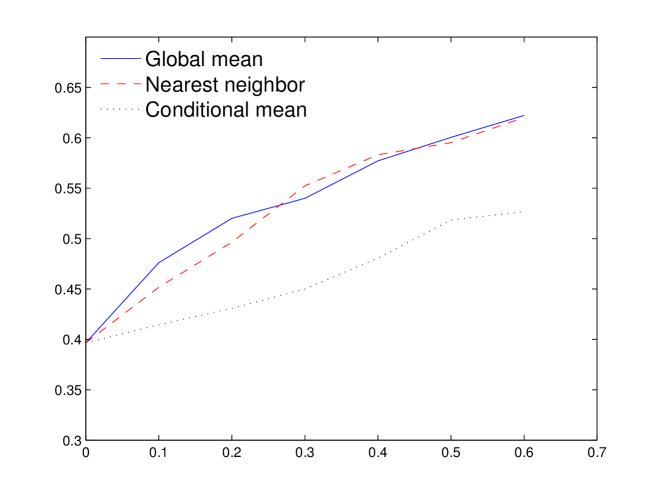
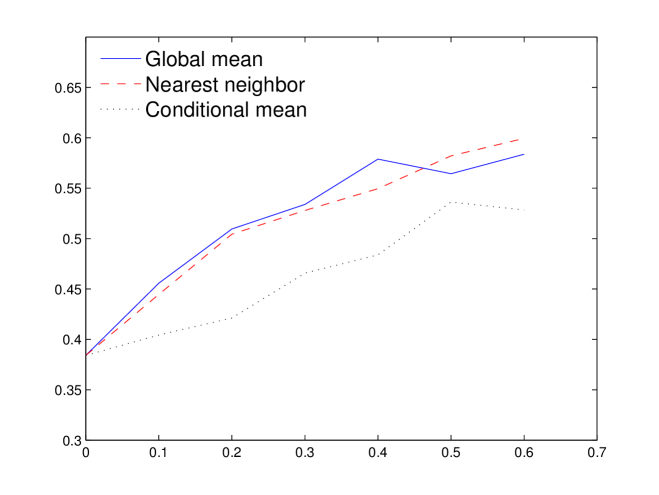
Figure 2: Test mean-squared error ($y$ axis) on Abalone when the proportion of missing values increases ($x$ axis). The three missing values imputation mechanisms are compared when using a neural network (top), and kernel ridge regression (bottom).

Figure 2 compares the three missing values imputation mechanisms when using a neural network and kernel ridge regression. It can be seen that the conditional mean imputation obtained by the Gaussian mixture significantly outperforms the global mean imputation and nearest neighbor imputation (which is tried with both 1 and 10 neighbors, keeping the best on the validation set). The latter seems to be reliable only when there are few missing values in the dataset: this is expected, as when the number of missing values increases one has to go further in space to find neighbors that contain non-missing values for the desired variables.

Figure 3 illustrates the gain of combining the generative model (the mixture of Gaussian) with the discriminant learning algorithms: even though the mixture can be used directly as a regressor (as argued in the introduction), its prediction accuracy can be greatly improved by a supervised learning step.

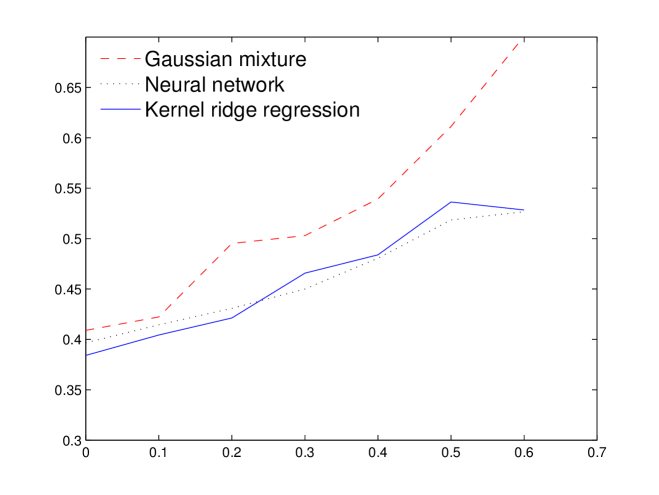
Figure 3: Test mean-squared error ($y$ axis) on Abalone when the proportion of missing values increases ($x$ axis). Combining a discriminant algorithm with the generative Gaussian mixture model works better than the Gaussian mixture alone (both the neural network and the kernel ridge regressor use here the conditional mean imputation of missing values provided by the Gaussian mixture).

V Conclusion

In this paper, we considered the problem of training Gaussian mixtures in the context of large high-dimensional datasets with a significant fraction of the data matrix missing. In such situations, the application of EM to the imputation of missing values results in expensive matrix computations. We have proposed a more efficient algorithm that uses matrix updates over a minimum spanning tree of missing patterns to speed-up these matrix computations, by an order of magnitude.

We also explored the application of a hybrid scheme where a mixture of Gaussians generative model, trained with EM, is used to impute the missing values with their conditional means. These imputed datasets were then used in a discriminant learning model (neural networks and kernel ridge regression) where they were shown to provide significant improvement over more basic missing value imputation methods.

References

- [1]
- [2] E. Parzen, “On the estimation of a probability density function and mode,” Annals of Mathematical Statistics, vol. 33, pp. 1064–1076, 1962.
- [3] A. P. Dempster, N. M. Laird, and D. B. Rubin, “Maximum-likelihood from incomplete data via the EM algorithm,” Journal of Royal Statistical Society B, vol. 39, pp. 1–38, 1977.
- [4] Z. Ghahramani and M. I. Jordan, “Supervised learning from incomplete data via an EM approach,” in Advances in Neural Information Processing Systems 6 (NIPS’93), D. Cowan, G. Tesauro, and J. Alspector, Eds. San Mateo, CA: Morgan Kaufmann, 1994.
- [5] L. Bahl, P. Brown, P. deSouza, and R. Mercer, “Maximum mutual information estimation of hidden markov parameters for speech recognition,” in International Conference on Acoustics, Speech and Signal Processing (ICASSP), Tokyo, Japan, 1986, pp. 49–52.
- [6] T. I. Lin, J. C. Lee, and H. J. Ho, “On fast supervised learning for normal mixture models with missing information,” Pattern Recognition, vol. 39, no. 6, pp. 1177–1187, Jun. 2006.
- [7] M. D. Zio, U. Guarnera, and O. Luzi, “Imputation through finite Gaussian mixture models,” Computational Statistics & Data Analysis, vol. 51, no. 11, pp. 5305–5316, 2007.
- [8] R. J. A. Little and D. B. Rubin, Statistical Analysis with Missing Data, 2nd ed. New York: Wiley, 2002.
- [9] M. Seeger, “Low rank updates for the Cholesky decomposition,” Department of EECS, University of California at Berkeley, Tech. Rep., 2005.
- [10] G. W. Stewart, Matrix Algorithms, Volume I: Basic Decompositions. Philadelphia: SIAM, 1998.
- [11] J. Whittaker, Graphical Models in Applied Multivariate Statistics. Wiley, Chichester, 1990.
- [12] F. K. Hwang, D. Richards, and P. Winter, “The Steiner tree problem,” Annals of Discrete Mathematics, vol. 53, 1992.
- [13] R. Caruana, “A non-parametric EM-style algorithm for imputing missing values,” in Proceedings of the Eigth International Workshop on Artificial Intelligence and Statistics (AISTATS’01). Society for Artificial Intelligence and Statistics, 2001.