An Improved Bound for the Nyström Method for Large Eigengap

Abstract

We develop an improved bound for the approximation error of the Nyström method under the assumption that there is a large eigengap in the spectrum of kernel matrix. This is based on the empirical observation that the eigengap has a significant impact on the approximation error of the Nyström method. Our approach is based on the concentration inequality of integral operator and the theory of matrix perturbation. Our analysis shows that when there is a large eigengap, we can improve the approximation error of the Nyström method from $O(N/m^{1/4})$ to $O(N/m^{1/2})$ when measured in Frobenius norm, where $N$ is the size of the kernel matrix, and $m$ is the number of sampled columns.

1 Introduction

The Nyström method has been used in kernel learning to approximate large kernel matrices (Fowlkes et al., 2004a; Platt, 2004; Kumar et al., 2009; Zhang et al., 2008; Williams & Seeger, 2001; Cortes et al., 2010; Talwalkar et al., 2008; Drineas & Mahoney, 2005; Silva & Tenenbaum, 2003; Belabbas & Wolfe, 2009; Talwalkar & Rostamizadeh, 2010). In order to evaluate the quality of Nyström method, we typically bound the norm of the difference between the original kernel matrix and the low rank approximation created by the Nyström method. Both the Frobenius norm and the spectral norm have been used to bound the difference between matrices (Drineas & Mahoney, 2005). The key result from (Drineas & Mahoney, 2005) is that besides the intrinsic error due to the low rank approximation, the additional error caused by the Nyström method is $O(N/m^{1/4})$ when measured in Frobenius norm, provided that the diagonal elements of kernel matrix is bounded by a constant. In this work, we consider the case when there is a large eigengap in the spectrum of the kernel matrix, a scenario that has been examined in many studies of kernel learning (Bach & Jordan, 2003; Luxburg, 2007; Azran & Ghahramani, 2006; Shi et al., 2009). Given sufficiently large eigengap, we are able to improve the bound for the additional approximation error caused by the Nyström method to $O(N/m^{1/2})$ when measured in Frobenius norm. The key techniques used in our analysis are the concentration inequality of integral operator (Smale & Zhou, 2009) and matrix perturbation theory (Stewart & guang Sun, 1990).

Our paper is structured as follows: in section 2, we demonstrate a discrepancy between the theoretical and experimental approximation error of the Nyström method that motivates our work to improve the existing bounds. Section 3 introduces the problem formally and proves the bounds. Finally, section 4 concludes the paper.

2 Background and Motivation

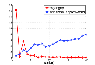
(a) MNIST

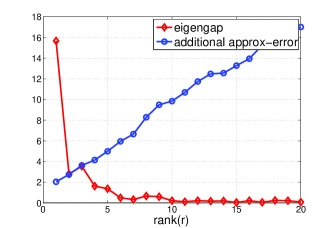
(b) a7a

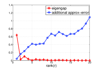
(c) diabetes

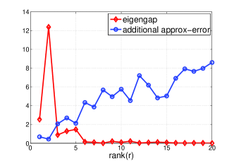
(d) CPU

Figure 1: Additional approximation error $\|K-\widehat{K}_{r}\|_{F}-\|K-K_{r}\|_{F}$ and eigengap $\lambda_{r}-\lambda_{r+1}$. Both the additional approximation error and eigengap are scaled appropriately so that they fall into the same range.

The Nyström method was first suggested in (Williams & Seeger, 2001) to improve the computational efficiency of Gaussian process. It was then adopted by a number of studies to improve the computational efficiency of kernel learning  (Fowlkes et al., 2004a; Platt, 2004; Kumar et al., 2009; Zhang et al., 2008; Talwalkar et al., 2008; Drineas & Mahoney, 2005; Silva & Tenenbaum, 2003; Cortes et al., 2010; Belabbas & Wolfe, 2009; Talwalkar & Rostamizadeh, 2010). Several analysis have been presented to bound the approximation error by the Nyström method (Drineas & Mahoney, 2005; Kumar et al., 2009; Belabbas & Wolfe, 2009; Talwalkar & Rostamizadeh, 2010). Most of them are based on the result from (Drineas & Mahoney, 2005) except for (Talwalkar & Rostamizadeh, 2010) whose analysis is limited to low rank kernel matrices and does not apply to the general case.

Let $K\in\mathbb{R}^{N\times N}$ be the kernel matrix to be approximated. Let $K_{r}$ be the $r$-rank best approximation of kernel matrix $K$, and let $\widehat{K}_{r}$ be an approximate kernel matrix of rank $r$ generated by the Nyström method. Assume $K_{i,i}\leq 1$ for any $i\in[N]$. Let $m$ be the number of columns uniformly sampled from $K$ used to construct $\widehat{K}_{r}$. Both Frobenius norm and spectral norm are used to bound the difference between $K$ and $\widehat{K}_{r}$. We note that it is important to derive the approximation errors measured in both norms as they have different implications. According to (Cortes et al., 2010), the approximation error measured in spectral norm is closely related to the generalized performance of kernel classifiers. On the other hand, the approximation error measured in Frobenius norm have found applications in kernel PCA Schölkopf et al. (1998), low dimensional manifold embedding Belkin & Niyogi (2001), spectral clustering Fowlkes et al. (2004b); Chitta et al. (2011). Improving the bound in the Frobenius norm will help us better understand the application of the Nyström method to those domains.

Drineas & Mahoney (2005) shows that with a high probability, we have

$$\|K-\widehat{K}_{r}\|_{2} \leq \|K-K_{r}\|_{2}+O\left(\frac{N}{\sqrt{m}}\right),$$ (1)

$$\|K-\widehat{K}_{r}\|_{F} \leq \|K-K_{r}\|_{F}+O\left(\frac{N}{m^{1/4}}\right),$$ (2)

where $\|\cdot\|_{2}$ and $\|\cdot\|_{F}$ stand for the spectral norm and Frobenius norm of a matrix, respectively. Compared to the bound in spectral norm in (1), the bound measured in Frobenius norm is significantly worse in terms of $m$, with the convergence rate of $O(m^{-1/4})$. The difference between the two bounds in (1) and (2) leads to the following question:

Under what scenario it is possible to improve the convergence rate of the bound in Frobenius norm to that of the bound measured in the spectral norm.

To this end, we first examine empirically the additional approximation error $\|K-\widehat{K}_{r}\|_{F}-\|K-K_{r}\|_{F}$. Note that we intentionally remove $\|K-K_{r}\|_{F}$ from the approximation error because $\|K-K_{r}\|_{F}$ provides the lower bound for any approximation with matrix of rank $r$. Four UCI datasets are used in this empirical study, i.e., MNIST, a7a, diabetes, CPU. The RBF kernel $\kappa(\mathbf{x},\mathbf{x}^{\prime})=\exp(-\lambda\|\mathbf{x}-\mathbf{x}^{\prime}\|_{2}^{2}/d^{2})$ is used, where $d^{2}$ is the average distance square between any two examples and $\lambda=10$. The blue curves with legend $\circ$ in Figure 1 show how the additional approximation error $\|K-\widehat{K}_{r}\|_{F}-\|K-K_{r}\|_{F}$ varies according to the rank $r$. The overall trend, as indicated in Figure 1, is that the higher the rank, the larger the additional approximation error tends to be. In order to explain the dependence of the approximation error on rank, we examine the distribution of eigengap $\lambda_{r}-\lambda_{r+1}$ over the rank. The red curves with legend $\diamond$ in Figure 1 show how the eigengap $\lambda_{r}-\lambda_{r+1}$ varies over the rank. Overall, we observe that the larger the rank, the smaller the eigengap. By combining the two observations, we conjecture that there is a strong dependence between the eigengap and the approximation error of the Nyström method. This motivates us to develop an eigengap dependent approximation error bound for the Nyström method. Our analysis show that when the eigengap $\lambda_{r}-\lambda_{r+1}$ is sufficiently large, the approximation error of the Nyström method, measured in Frobenius norm, can be improved to $O(N/\sqrt{m})$, i.e.

$$\|K-\widehat{K}_{r}\|_{F}\leq\|K-K_{r}\|_{F}+O\left(\frac{N}{\sqrt{m}}\right).$$

We note that although the concept of eigengap has been exploited in many studies of kernel learning (Bach & Jordan, 2003; Luxburg, 2007; Azran & Ghahramani, 2006; Shi et al., 2009), to the best of our knowledge, this is the first time it has been incorporated in the analysis of the Nyström method.

In the development of the Nyström method, another important issue is how to sample the columns in the kernel matrix. We restrict our analysis to the uniform sampling. Although different sampling approaches have been suggested for the Nyström method (Drineas & Mahoney, 2005; Kumar et al., 2009; Zhang et al., 2008; Belabbas & Wolfe, 2009), according to (Kumar et al., 2009), for real-world datasets, uniform sampling seems to be the most efficient and gives comparable performance to the other sampling approaches. We notice that in (Belabbas & Wolfe, 2009), the authors show a significantly better approximation bound for the Nyström method, both theoretically and empirically, when sampling the columns based on the determinant of the submatrix formed by the selected columns and rows, which is also referred to as determinantal processes (Hough et al., 2006). It is however important to point out that the determinantal process is usually computationally expensive as it requires computing the determinant of the submatrix for the selected columns/rows, making it unsuitable for the case when a large number of columns are needed to be sampled.

3 Approximation Error Bound by the Nyström Method

Let $\mathcal{D}=\{\mathbf{x}_{1},\ldots,\mathbf{x}_{N}\}$ be a collection of $N$ samples, and $K=[\kappa(\mathbf{x}_{i},\mathbf{x}_{j})]_{N\times N}$ be the kernel matrix for the samples in $\mathcal{D}$, where $\kappa(\cdot,\cdot)$ is a kernel function. For simplicity, we assume $\kappa(\mathbf{x},\mathbf{x})\leq 1$ for any $\mathbf{x}\in\mathcal{X}$. Let $\mathcal{H}_{\kappa}$ be the Reproducing Kernel Hilbert Space (RKHS) endowed with kernel $\kappa(\cdot,\cdot)$. We denote by $(\mathbf{v}_{i},\lambda_{i}),i=1,\ldots,N$ the eigenvectors and eigenvalues of $K$ ranked in the descending order of eigenvalues. Define $V=(\mathbf{v}_{1},\cdots,\mathbf{v}_{N})$ and $V_{i,j}=[V]_{i,j}$. In order to build the low rank approximation of kernel matrix $K$ of rank $r$, the Nyström method first samples $m<N$ examples randomly from $\mathcal{D}$, denoted by $\widehat{\mathcal{D}}=\left\{\widehat{\mathbf{x}}_{1},\ldots,\widehat{\mathbf{x}}_{m}\right\}$. It then computes a sample kernel matrix $\widehat{K}=[\kappa(\widehat{\mathbf{x}}_{i},\widehat{\mathbf{x}}_{j})]_{m\times m}$. Let $(\mathbf{u}_{i},\widehat{\lambda}_{i}),i=1,\ldots,r$ be the first $r$ eigenvalues and eigenvectors of matrix $\widehat{K}$, and let $U=(\mathbf{u}_{1},\cdots,\mathbf{u}_{r})$, $U_{i,j}=[U]_{i,j}$. We assume $\widehat{\lambda}_{r}>0$ is strictly positive and define matrix $\widehat{W}$ as

$$\widehat{W}=\sum_{i=1}^{r}\frac{1}{\widehat{\lambda}_{i}}\mathbf{u}_{i}\mathbf{u}_{i}^{\top}.$$

The approximate low rank matrix $\widehat{K}_{r}$, computed by the Nyström method, is given by

$$\widehat{K}_{r}=K_{b}\widehat{W}K_{b}^{\top},$$

where $K_{b}=[\kappa(\mathbf{x}_{i},\widehat{\mathbf{x}}_{j})]_{N\times m}$ measures the similarity between the samples in $\mathcal{D}$ and $\widehat{\mathcal{D}}$. As already mentioned, we focus on the scenario when the eigengap $\lambda_{r}-\lambda_{r+1}$ is sufficiently large . Our analysis is mainly based on the concentration inequality of integral operator (Smale & Zhou, 2009) and matrix perturbation theory (Stewart & guang Sun, 1990).

3.1 Preliminaries

We define an integral operator $L_{N}$ and $L_{m}$ based on the samples in $\mathcal{D}$ and $\widehat{\mathcal{D}}$, respectively, as

$$L_{N}[f](\cdot)=\frac{1}{N}\sum_{i=1}^{N}\kappa(\mathbf{x}_{i},\cdot)f(\mathbf{x}_{i}),$$

$$L_{m}[f](\cdot)=\frac{1}{m}\sum_{i=1}^{m}\kappa(\widehat{\mathbf{x}}_{i},\cdot)f(\widehat{\mathbf{x}}_{i}),$$

where $f\in\mathcal{H}_{\kappa}$ is any function in $\mathcal{H}_{\kappa}$. The eigenvalues of the integral operator $L_{N}$ and $L_{m}$, according to (Smale & Zhou, 2009), are $\lambda_{i}/N,i\in[N]$ and $\widehat{\lambda}_{i}/m,i\in[m]$, respectively. Let $\varphi_{1}(\cdot),\ldots,\varphi_{N}(\cdot)$ be the corresponding eigenfunctions of $L_{N}$ that are normalized by functional norm, i.e., $\langle\varphi_{i},\varphi_{j}\rangle_{\mathcal{H}_{\kappa}}=\delta(i,j),\quad\forall(i,j)\in[N]\times[N]$. According to (Smale & Zhou, 2009), the eigenfunctions are given by

$$\varphi_{j}(\cdot)=\frac{1}{\sqrt{\lambda_{j}}}\sum_{i=1}^{N}V_{i,j}\kappa(\mathbf{x}_{i},\cdot),j\in[N].$$ (3)

Using the eigenfunctions expressed in (3), we can write $\kappa(\mathbf{x}_{j},\cdot),j\in[N]$ as

$$\kappa(\mathbf{x}_{j},\cdot) =\sum_{i=1}^{N}\sqrt{\lambda_{i}}V_{j,i}\varphi_{i}(\cdot)=\sum_{i=1}^{N}\langle\kappa(\mathbf{x}_{j},\cdot),\varphi_{i}\rangle\varphi_{i}.$$ (4)

It is easy to verify that $L_{N}$ can be written in the base of $\varphi_{i},i\in[N]$ by

$$L_{N}(f)(\cdot)=\frac{1}{N}\sum_{i=1}^{N}\lambda_{i}\varphi_{i}\langle f,\varphi_{i}\rangle_{\mathcal{H}_{\kappa}}.$$ (5)

Let $\widehat{\varphi}_{j},j\in[m]$ be the corresponding eigenvectors of the integral operator $L_{m}$. Similar to $L_{N}$, the eigenfunction $\widehat{\varphi}_{i}$ is given by

$$\widehat{\varphi}_{j}(\cdot)=\frac{1}{\sqrt{\widehat{\lambda}_{j}}}\sum_{i=1}^{m}U_{i,j}\kappa(\widehat{\mathbf{x}}_{i},\cdot).$$ (6)

We define the Hilbert Schmidt norm of operator $L:\mathcal{H}_{k}\rightarrow\mathcal{H}_{k}$ by

$$\|L\|_{HS}=\sqrt{\sum_{i,j=1}^{N}\langle\varphi_{i},L\varphi_{j}\rangle_{\mathcal{H}_{\kappa}}^{2}}.$$ (7)

Let $\|L\|_{2}$ denote the spectral norm of operator $L$ defined by

$$\|L\|_{2}=\max_{\|f\|_{\mathcal{H}_{\kappa}}\leq 1}\langle f,Lf\rangle_{\mathcal{H}_{\kappa}}.$$

where $\langle\cdot,\cdot\rangle_{\mathcal{H}_{\kappa}}$ denotes the inner product in Hilbert space $\mathcal{H}_{\kappa}$. In the sequel, we use $\langle\cdot,\cdot\rangle$ for short.

We state the concentration inequality about the two integral operators in the following.

Lemma 1.

(Proposition 1 (Smale & Zhou, 2009)) Let $\xi$ be a random variable on $(\mathcal{X},P_{\mathcal{X}})$ with values in a Hilbert space $(\mathcal{H},\|\cdot\|)$. Assume $\|\xi\|\leq M<\infty$ almost sure. Then with a probability at least $1-\delta$, we have

$$\left\|\frac{1}{m}\sum_{i=1}^{m}\xi(\mathbf{x}_{i})-\mathrm{E}[\xi]\right\|\leq\frac{4M\ln(2/\delta)}{\sqrt{m}}.$$

Theorem 1.

With a probability $1-\delta$, we have

$$\|L_{N}-L_{m}\|_{HS}\leq\frac{4\ln(2/\delta)}{\sqrt{m}},$$

where $\|L\|_{HS}$ is defined in equation (7).

Proof.

Define $\xi(\widehat{\mathbf{x}}_{i})$ as a rank one linear operator, i.e.,

$$\xi(\widehat{\mathbf{x}}_{i})[f](\cdot)=\kappa(\widehat{\mathbf{x}}_{i},\cdot)f(\widehat{\mathbf{x}}_{i}).$$

Apparently, $L_{m}=\frac{1}{m}\sum_{i=1}^{m}\xi(\widehat{\mathbf{x}}_{i})$ and $\mathrm{E}[\xi(\widehat{\mathbf{x}}_{i})]=L_{N}$. Let $\|\cdot\|_{HS}$ be the norm used in Lemma 1. We complete the proof by using the result from Lemma 1 and the fact

$$\|\xi(\widehat{\mathbf{x}}_{k})\|_{HS} =\sqrt{\sum_{i,j=1}^{N}\langle\varphi_{i},\kappa(\widehat{\mathbf{x}}_{k},\cdot)\varphi_{j}(\widehat{\mathbf{x}}_{k})\rangle^{2}}$$

$$=\sqrt{\sum_{i,j=1}^{N}\varphi_{i}(\widehat{\mathbf{x}}_{k})^{2}\varphi_{j}(\widehat{\mathbf{x}}_{k})^{2}}=\kappa(\widehat{\mathbf{x}}_{k},\widehat{\mathbf{x}}_{k})\leq 1,$$

where the last equality follows equation (4). ∎

3.2 Bounding the Approximation Error by Operator Norm

Based on the first $r$ eigenfunctions of $L_{N}$ and $L_{m}$, we define two additional linear operators $H_{r}$ and $\widehat{H}_{r}$ as

$$H_{r}[f](\cdot)=\sum_{i=1}^{r}\varphi_{i}(\cdot)\langle\varphi_{i},f\rangle,$$

$$\widehat{H}_{r}[f](\cdot)=\sum_{i=1}^{r}\widehat{\varphi}_{i}(\cdot)\langle\widehat{\varphi}_{i},f\rangle.$$

The following lemma relates $H_{r}$ and $\widehat{H}_{r}$ to matrices $K_{r}$ and $\widehat{K}_{r}$, respectively.

Proposition 1.

Assume $\widehat{\lambda}_{r}>0$ and $\lambda_{r}>0$. We have for any $(i,j)\in[N]\times[N]$

$$\left[\widehat{K}_{r}\right]_{i,j}=\langle\kappa(\mathbf{x}_{i},\cdot),\widehat{H}_{r}\kappa(\mathbf{x}_{j},\cdot)\rangle,$$

$$\left[K_{r}\right]_{i,j}=\langle\kappa(\mathbf{x}_{i},\cdot),H_{r}\kappa(\mathbf{x}_{j},\cdot)\rangle.$$

Proof.

By the definition of $\widehat{H}_{r}$ and equation (6), we have

$$\langle\kappa(\mathbf{x}_{i},\cdot),\widehat{H}_{r}\kappa(\mathbf{x}_{j},\cdot)\rangle$$

$$=\sum_{k=1}^{r}\frac{1}{\widehat{\lambda}_{k}}\langle\kappa(\mathbf{x}_{i},\cdot),\widehat{\varphi}_{k}\rangle\langle\kappa(\mathbf{x}_{j},\cdot),\widehat{\varphi}_{k}\rangle$$

$$=\sum_{a,b=1}^{m}\sum_{k=1}^{r}\frac{1}{\widehat{\lambda}_{k}}U_{a,k}U_{b,k}\langle\kappa(\mathbf{x}_{i},\cdot),\kappa(\widehat{\mathbf{x}}_{a},\cdot)\rangle\langle\kappa(\mathbf{x}_{j},\cdot),\kappa(\widehat{\mathbf{x}}_{b},\cdot)\rangle$$

$$=\sum_{a,b=1}^{m}\sum_{k=1}^{r}\frac{U_{a,k}U_{b,k}}{\widehat{\lambda}_{k}}[K_{b}]_{i,a}[K_{b}]_{j,b}$$

$$=\sum_{a,b=1}^{m}[K_{b}]_{i,a}\widehat{W}_{a,b}[K_{b}]_{j,b}=[K_{b}\widehat{W}K_{b}^{\top}]_{i,j}=[\widehat{K}_{r}]_{i,j}.$$

Using the fact that $K_{r}=KWK$, where

$$W=\sum_{i=1}^{r}\frac{1}{\lambda_{i}}\mathbf{v}_{i}\mathbf{v}_{i}^{\top},$$

we apply the same proof to $K_{r}$. ∎

Next, we will relate $\|K_{r}-\widehat{K}_{r}\|_{F}$ to $\Delta H=H_{r}-\widehat{H}_{r}$. Note that $L_{N}$ and $H_{r},\widehat{H}_{r}$ are self-adjoint operators, and so is $\Delta H$. In the proof of Theorem 2, we repeatedly use

$$\langle f,\Delta Hg\rangle =\langle\Delta Hf,g\rangle,$$

$$NL_{N}(f) =\sum_{i=1}^{N}\kappa(\mathbf{x}_{i},\cdot)\langle f,\kappa(\mathbf{x}_{i},\cdot)\rangle.$$

Theorem 2.

Assume $\widehat{\lambda}_{r}>0$ and $\lambda_{r}>0$. We have

$$\|\widehat{K}_{r}-K_{r}\|_{F}\leq\sqrt{\lambda_{1}N}\|\Delta H\|_{2}\leq N\|\Delta H\|_{2}.$$

The proof can be found in the Appendix A. As indicated by Theorem 2, to bound $\|\widehat{K}_{r}-K_{r}\|_{F}$, the key is to bound the spectral norm of operator $\Delta H$.

3.3 Bounding the Operator Norm by Matrix Perturbation Theory

Our next goal is to bound the spectral norm of $\Delta H$. To this end, we assume a large eigengap between $\lambda_{r}$ and $\lambda_{r+1}$, i.e., $\Delta=(\lambda_{r}-\lambda_{r+1})/N$ is sufficiently large. Note that we normalize $\lambda_{r}-\lambda_{r+1}$ by $N$, the size of dataset $\mathcal{D}$, when defining $\Delta$. Eigengap has the key quantity for the application of matrix perturbation theory (Stewart & guang Sun, 1990). The following perturbation result from (Stewart & guang Sun, 1990) forms the foundation of our analysis .

Theorem 3.

(Theorem 2.7 of Chapter 6 (Stewart & guang Sun, 1990)) Let $(\lambda_{i},\mathbf{v}_{i}),i\in[n]$ be the eigenvalues and eigenvectors of a symmetric matrix $A\in\mathbb{R}^{n\times n}$ ranked in the descending order of eigenvalues. Set $X=(\mathbf{v}_{1},\ldots,\mathbf{v}_{r})$ and $Y=(\mathbf{v}_{r+1},\ldots,\mathbf{v}_{n})$. Given a symmetric perturbation matrix $E$, let

$$\widehat{E}=(X,Y)^{\top}E(X,Y)=\left(\begin{array}[]{cc}\widehat{E}_{11}&\widehat{E}_{12}\\ \widehat{E}_{21}&\widehat{E}_{22}\end{array}\right).$$

Let $\|\cdot\|$ represent a consistent family of norms and set

$$\gamma=\|\widehat{E}_{21}\|,\delta=\lambda_{r}-\lambda_{r+1}-\|\widehat{E}_{11}\|-\|\widehat{E}_{22}\|$$

If $\delta>0$ and $2\gamma<\delta$, then there exists a unique matrix $P\in\mathbb{R}^{(n-r)\times r}$ satisfying $\|P\|<\frac{2\gamma}{\delta}$ such that

$$X^{\prime} =(X+YP)(I+P^{\top}P)^{-1/2},$$

$$Y^{\prime} =(Y-XP^{\top})(I+PP^{\top})^{-1/2},$$

are the eigenvectors of $A+E$.

Define

$$\Theta =\left(\widehat{\varphi}_{1},\ldots,\widehat{\varphi}_{r}\right),$$

$$\Phi =\left(\varphi_{1},\ldots,\varphi_{r}\right),\overline{\Phi}=\left(\varphi_{r+1},\ldots,\varphi_{N}\right).$$

The following theorem allows us to relate $\Theta$ with $\Phi$ and $\overline{\Phi}$.

Theorem 4.

Assume

$$\Delta=\frac{\lambda_{r}-\lambda_{r+1}}{N}>3\|L_{N}-L_{m}\|_{HS}.$$

Then, there exists a matrix $P\in\mathbb{R}^{(N-r)\times r}$ satisfying

$$\|P\|_{F}\leq\frac{2\|L_{N}-L_{m}\|_{HS}}{\Delta-\|L_{N}-L_{m}\|_{HS}}\leq\frac{3\|L_{N}-L_{m}\|_{HS}}{\Delta},$$

such that

$$\Theta=(\Phi+\overline{\Phi}P)(I+P^{\top}P)^{-1/2}.$$

The proof can be found in Appendix B. As indicated by Theorem 4, when the eigengap $\Delta$ is sufficiently large, we have a small $\|P\|_{F}$ and therefore $\Theta\approx\Phi$, implying that the eigenfunctions $\{\widehat{\varphi}_{i}\}_{i=1}^{r}$, computed based on the samples in $\widehat{\mathcal{D}}$, are good approximation of $\{\varphi_{i}\}_{i=1}^{r}$, the eigenfunctions of $L_{N}$. As a result, when the eigengap $\Delta$ is sufficiently large, we expect a small difference between $H_{r}$ and $\widehat{H}_{r}$ because they are constructed based on eigenfunctions $\{\varphi_{i}\}_{i=1}^{r}$ and $\{\widehat{\varphi}_{i}\}_{i=1}^{r}$, respectively. This is shown in the next theorem.

Theorem 5.

Assume

$$\Delta=\frac{\lambda_{r}-\lambda_{r+1}}{N}>3\|L_{N}-L_{m}\|_{HS}.$$

We have

$$\|\Delta H\|_{2}\leq\frac{4\|L_{N}-L_{m}\|_{HS}}{\Delta-\|L_{N}-L_{m}\|_{HS}}\leq\frac{6\|L_{N}-L_{m}\|_{HS}}{\Delta}.$$

The proof can be found in Appendix C. By putting the results from Theorem 1, 2 and 5, we have the final theorem for the approximation of the Nyström method measured in Frobenious norm.

Theorem 6.

Assume

$$\Delta=\frac{\lambda_{r}-\lambda_{r+1}}{N}>3\|L_{N}-L_{m}\|_{HS}.$$

We have

$$\|K_{r}-\widehat{K}_{r}\|_{F}\leq\frac{4N\|L_{N}-L_{m}\|_{HS}}{\Delta-\|L_{N}-L_{m}\|_{HS}}\leq\frac{6N\|L_{N}-L_{m}\|_{HS}}{\Delta}.$$

If the eigengap satisfies

$$\Delta=\Omega(1)>\frac{12\ln(2/\delta)}{\sqrt{m}},$$

then, with a probability $1-\delta$, we have

$$\|K_{r}-\widehat{K}_{r}\|_{F}\leq O\left(\frac{N}{\sqrt{m}}\right).$$

Proof.

The proof is simply the combination of the results from Theorem 1, 2 and 5.

$$\|K_{r}-\widehat{K}_{r}\|_{F}\leq N\|\Delta H\|_{2}\leq\frac{4N\|L_{N}-L_{m}\|_{HS}}{\Delta-\|L_{N}-L_{m}\|_{HS}}$$

$$\leq\frac{6N\|L_{N}-L_{m}\|_{HS}}{\Delta}\leq O\left(\frac{N}{\sqrt{m}}\right),$$

where the third inequality follows $\|L_{N}-L_{m}\|_{HS}\leq\Delta/3$ and the last inequality follows from Theorem 2. Note that both conditions $\lambda_{r}>0$ and $\widehat{\lambda}_{r}>0$, specified in Theorem 2, hold with a high probability. It is obvious that $\lambda_{r}>0$ because $\lambda_{r}>\lambda_{r+1}$ and $\lambda_{r+1}\geq 0$. To show $\widehat{\lambda}_{r}>0$ holds with a high probability, we use the Lidskii’s inequality (Koltchinskii & Gine, 2000), i.e.,

$$\widehat{\lambda}_{r}\geq\lambda_{r}-N\|L_{N}-L_{m}\|_{HS}.$$

Since with a probability $1-\delta$, $\lambda_{r}-\lambda_{r+1}\geq 3N\|L_{N}-L_{m}\|_{HS}$ holds, we have, with a probability $1-\delta$

$$\widehat{\lambda}_{r}\geq\lambda_{r}-\frac{\lambda_{r}-\lambda_{r+1}}{3}=\frac{2}{3}\lambda_{r}+\frac{1}{3}\lambda_{r+1}>0.$$

∎

Remark

Besides the improved bound for the Nyström method, Theorem 6 also explains the results shown in Figure 1. Since the additional approximation error $\|K-K_{r}\|_{F}-\|K-\widehat{K}_{r}\|_{F}$ is upper bounded by $\|K_{r}-\widehat{K}_{r}\|_{F}$, according to Theorem 6, we would expect the additional approximation error bound to be inversely related to the eigengap $\lambda_{r}-\lambda_{r+1}$, i.e. the larger the eigengap, the smaller the additional approximation error.

4 Conclusion

In this paper we tried to bridge the gap between effectiveness of Nyström method in practice and its poor theoretical approximation error bounds. In particular, in the case of large eigengap, we developed an improved bound for the approximation error of the Nyström method, based on the concentration inequality and the theory of matrix perturbation. In the future, we plan to develop better bounds for the Nyström method that take into account the eigenvalues of kernel matrix which follow a power law.

Appendix A: Proof of Theorem 2

Since $K_{r}=KWK$ and $\widehat{K}_{r}=K_{b}\widehat{W}K_{b}^{\top}$, we have

$$\|KWK-K_{b}\widehat{W}K_{b}^{\top}\|_{F}^{2}$$

$$=\sum_{i,j=1}^{N}([KWK]_{i,j}-[K_{b}\widehat{W}K_{b}^{\top}]_{i,j})^{2}$$

$$=\sum_{i,j=1}^{N}\langle\kappa(\mathbf{x}_{i},\cdot),(H_{r}-\widehat{H}_{r})\kappa(\mathbf{x}_{j},\cdot)\rangle^{2}$$

$$=\sum_{i,j=1}^{N}\langle\Delta H\kappa(\mathbf{x}_{i},\cdot),\kappa(\mathbf{x}_{j},\cdot)\rangle\langle\Delta H\kappa(\mathbf{x}_{i},\cdot),\kappa(\mathbf{x}_{j},\cdot)\rangle.$$

Using the fact $\sum_{j=1}^{N}\langle f,\kappa(\mathbf{x}_{j},\cdot)\rangle\langle f,\kappa(\mathbf{x}_{j},\cdot)\rangle=N\langle f,L_{N}f\rangle$, we have

$$\|KWK-K_{b}\widehat{W}K_{b}^{\top}\|_{F}^{2}$$

$$=N\sum_{i=1}^{N}\left\langle\Delta H\kappa(\mathbf{x}_{i},\cdot),L_{N}\Delta H\kappa(\mathbf{x}_{i},\cdot)\right\rangle$$

$$=N\sum_{i=1}^{N}\langle\kappa(\mathbf{x}_{i},\cdot),\Delta HL_{N}\Delta H\kappa(\mathbf{x}_{i},\cdot)\rangle.$$

We further simplify the expression by using the fact that for any linear operator $Z$, we have

$$\sum_{i=1}^{N}\langle\kappa(\mathbf{x}_{i},\cdot),Z\kappa(\mathbf{x}_{i},\cdot)\rangle=N\sum_{i=1}^{N}\langle\varphi_{i},(ZL_{N})\varphi_{i}\rangle.$$

Using the above result with $Z=\Delta HL_{N}\Delta H$, we have

$$\|KWK-K_{b}\widehat{W}K_{b}^{\top}\|_{F}^{2}$$

$$=N^{2}\sum_{i=1}^{N}\langle\varphi_{i},(\Delta HL_{N}\Delta HL_{N})\varphi_{i}\rangle$$

$$=N\sum_{i=1}^{N}\lambda_{i}\langle\varphi_{i},(\Delta HL_{N}\Delta H)\varphi_{i}\rangle$$

$$\leq N\lambda_{1}\sum_{i=1}^{N}\langle\Delta H\varphi_{i},L_{N}\Delta H\varphi_{i}\rangle$$

$$=\lambda_{1}\sum_{i,j=1}^{N}\lambda_{j}\langle\varphi_{j},\Delta H\varphi_{i}\rangle^{2}_{\mathcal{H}_{\kappa}}=\lambda_{1}\sum_{i,j=1}^{N}\lambda_{j}\langle\varphi_{i},\Delta H\varphi_{j}\rangle^{2},$$

where the last one equality follows equation (5). Define a matrix $A=[\langle\varphi_{i},\Delta H\varphi_{j}\rangle]_{N\times N}$ and $D=\mbox{diag}(\lambda_{1},\ldots,\lambda_{N})$. We have

$$\|KWK-K_{b}\widehat{W}K_{b}^{\top}\|_{F}^{2}\leq\lambda_{1}\mbox{tr}(ADA)$$

$$\leq \lambda_{1}\|A\|_{2}^{2}\sum_{i=1}^{N}\lambda_{i}\leq\lambda_{1}N\|\Delta H\|_{2}^{2},$$

where the last step follows from $\|A\|_{2}=\|\Delta H\|_{2}$.

Appendix B: Proof of Theorem 4

Define matrix $B$ as

$$B_{i,j}=\frac{1}{m}\sum_{k=1}^{m}\widehat{\lambda}_{k}\langle\widehat{\varphi}_{k},\varphi_{i}\rangle\langle\widehat{\varphi}_{k},\varphi_{j}\rangle.$$

Let $\mathbf{z}_{i}$ be the eigenvector of $B$ corresponding to eigenvalue $\widehat{\lambda}_{i}/m$. It is straightforward to show that

$$\mathbf{z}_{i}=(\langle\varphi_{1},\widehat{\varphi}_{i}\rangle_{\mathcal{H}_{\kappa}},\ldots,\langle\varphi_{N},\widehat{\varphi}_{i}\rangle_{\mathcal{H}_{\kappa}})^{\top},i\in[m],$$

and therefore we have

$$\widehat{\varphi}_{i}=\sum_{k=1}^{N}z_{i,k}\varphi_{k},i\in[m],\mbox{ or }\Theta=(\Phi,\overline{\Phi})Z,$$

where $Z=(\mathbf{z}_{1},\cdots,\mathbf{z}_{r})$. To decide the relationship between $\{\widehat{\varphi}_{i}\}_{i=1}^{r}$ and $\{\varphi_{i}\}_{i=1}^{N}$, we need to determine matrix $Z$. We define matrix $D=\mbox{diag}(\lambda_{1}/N,\ldots,\lambda_{N}/N)$ and matrix $E=B-D$, i.e.

$$E_{i,j}=B_{i,j}-\lambda_{i}\delta_{i,j}/N=\langle\varphi_{i},(L_{m}-L_{N})\varphi_{j}\rangle_{\mathcal{H}_{\kappa}}.$$

Following the notation of Theorem 3, we define $X=(e_{1},\ldots,e_{r})$ and $Y=(e_{r+1},\ldots,e_{N})$, where $e_{1},\ldots,e_{N}$ are the canonical bases of $\mathbb{R}^{N}$, which are also eigenvectors of $D$. Define $\delta$ and $\gamma$ as follows

$$\gamma =\sqrt{\sum_{i=1}^{r}\sum_{j=r+1}^{N}\langle\varphi_{i},(L_{N}-L_{m})\varphi_{j}\rangle^{2}_{\mathcal{H}_{\kappa}}}$$

$$\delta =\Delta-\sqrt{\sum_{i,j=1}^{r}\langle\varphi_{i},(L_{N}-L_{m})\varphi_{j}\rangle^{2}_{\mathcal{H}_{\kappa}}}$$

$$\hskip 21.68121pt-\sqrt{\sum_{i,j=r+1}^{N}\langle\varphi_{i},(L_{N}-L_{m})\varphi_{j}\rangle^{2}_{\mathcal{H}_{\kappa}}}.$$

It is easy to verify that $\gamma,\delta$ are defined with respect to the Frobenius norm of $\widehat{E}$ in Theorem 3. In order to apply the result in Theorem 3, we need to show $\delta>0$ and $\gamma<\delta/2$. To this end, we need to provide the lower and upper bounds for $\gamma$ and $\delta$, respectively. We first bound $\delta$ as

$$\delta-\Delta \geq -\sqrt{\sum_{i,j=1}^{N}\langle\varphi_{i},(L_{N}-L_{m})\varphi_{j}\rangle_{\mathcal{H}_{\kappa}}^{2}}$$

$$= -\|L_{N}-L_{m}\|_{HS}.$$

We then bound $\gamma$ as

$$\gamma = \sqrt{\sum_{i=1}^{r}\sum_{j=r+1}^{N}\langle\varphi_{i},(L_{N}-L_{m})\varphi_{j}\rangle_{\mathcal{H}_{\kappa}}^{2}}$$

$$\leq \sqrt{\sum_{i=1}^{N}\sum_{j=1}^{N}\langle\varphi_{i},(L_{N}-L_{m})\varphi_{j}\rangle_{\mathcal{H}_{\kappa}}^{2}}$$

$$= \|L_{N}-L_{m}\|_{HS}.$$

Hence, when $\Delta>3\|L_{N}-L_{m}\|_{HS}$, we have $\delta>2\gamma>0$, which satisfies the condition specified in Theorem 3. Thus, according to Theorem 3, there exists a $P\in\mathbb{R}^{(N-r)\times r}$ satisfying $\|P\|<2\gamma/\delta$, such that

$$Z=(\mathbf{z}_{1},\ldots,\mathbf{z}_{r})=(X+YP)(I+P^{\top}P)^{-1/2},$$

implying

$$\Theta=(\Phi,\overline{\Phi})Z=(\Phi+\overline{\Phi}P)(I+P^{\top}P)^{-1/2}.$$

Appendix C: Proof of Theorem 5

To bound $\|\Delta H\|_{2}$, it is sufficient to bound $\max_{\|f\|_{\mathcal{H}_{\kappa}}\leq 1}\langle f,\Delta Hf\rangle$. Consider any function $f(\cdot)=\sum_{i=1}^{N}f_{i}\varphi_{i}(\cdot)$, with $\|f\|_{\mathcal{H}_{\kappa}}\leq 1$. Let $\mathbf{f}=(f_{1},\ldots,f_{N})^{\top}$. Evidently, we have $\|\mathbf{f}\|_{2}\leq 1$. We have

$$\langle f,\widehat{H}_{r}f\rangle= \sum_{i=1}^{r}\sum_{a,b=1}^{N}f_{a}f_{b}\langle\varphi_{a},\widehat{\varphi}_{i}\rangle\langle\varphi_{b},\widehat{\varphi}_{i}\rangle=\|A^{\top}\mathbf{f}\|_{2}^{2}$$

$$\langle f,H_{r}f\rangle= \sum_{i=1}^{r}\sum_{a,b=1}^{N}f_{a}f_{b}\langle\varphi_{a},\varphi_{i}\rangle\langle\varphi_{b},\varphi_{i}\rangle$$

$$=\mathbf{f}^{\top}\left(\begin{array}[]{cc}I_{r\times r}&0\\ 0&0\end{array}\right)\mathbf{f}.$$

where $A=[\langle\varphi_{i},\widehat{\varphi}_{j}\rangle_{\mathcal{H}_{\kappa}}]_{N\times m}=(\Phi,\overline{\Phi})^{\top}\Theta$. Since $\Delta>3\|L_{N}-L_{m}\|_{HS}$, according to Theorem 4, there exists an matrix $P\in\mathbb{R}^{(N-r)\times r}$ satisfying

$$\|P\|_{F}\leq\frac{2\|L_{N}-L_{m}\|_{HS}}{\Delta-\|L_{N}-L_{m}\|_{HS}},$$

such that

$$\Theta=\left(\Phi+\overline{\Phi}P\right)(I+P^{\top}P)^{-1/2}.$$

Using the expression of $\Theta$, we compute $A$ as

$$A =(\Phi,\overline{\Phi})^{\top}\Theta=(\Phi,\overline{\Phi})^{\top}\left(\Phi+\overline{\Phi}P\right)(I+P^{\top}P)^{-1/2}$$

$$=\left(\begin{array}[]{c}I\\ P\end{array}\right)(I+P^{\top}P)^{-1/2}.$$

Thus, we have

$$\langle f,\Delta Hf\rangle=\mathbf{f}^{\top}\left(\left(\begin{array}[]{cc}I&0\\ 0&0\end{array}\right)-AA^{\top}\right)\mathbf{f}=\mathbf{f}^{\top}C\mathbf{f},$$

where $C$ is given by

$$C =\left(\begin{array}[]{cc}I-(I+P^{\top}P)^{-1}&(I+P^{\top}P)^{-1}P^{\top}\\ P(I+P^{\top}P)^{-1}&-P(I+P^{\top}P)^{-1}P^{-1}\end{array}\right)$$

$$=\left(\begin{array}[]{cc}(I+P^{\top}P)^{-1}P^{\top}P&(I+P^{\top}P)^{-1}P^{\top}\\ P(I+P^{\top}P)^{-1}&-P(I+P^{\top}P)^{-1}P^{\top}\end{array}\right).$$

Rewrite $\mathbf{f}=(\mathbf{f}_{a},\mathbf{f}_{b})$ where $\mathbf{f}_{a}\in\mathbb{R}^{r}$ includes the first $r$ entries in $\mathbf{f}$ and $\mathbf{f}_{b}$ includes the rest of the entries in $\mathbf{f}$. We have

$$\mathbf{f}^{\top}C\mathbf{f}\leq\left(\|\mathbf{f}_{a}\|_{2}^{2}+\|\mathbf{f}_{b}\|_{2}^{2}\right)\|P(I+P^{\top}P)^{-1}P^{\top}\|_{2}$$

$$+2\|\mathbf{f}_{a}\|\|\mathbf{f}_{b}\|\left\|(I+P^{\top}P)^{-1}P\right\|_{2}$$

$$\leq(\|\mathbf{f}_{a}\|_{2}+\|\mathbf{f}_{b}\|_{2})^{2}\cdot$$

$$\hskip 7.22743pt\max\left(\left\|P(I+P^{\top}P)^{-1}P^{\top}\right\|_{2},\left\|(I+P^{\top}P)^{-1}P^{\top}\right\|_{2}\right)$$

$$\leq 2\max\left(\left\|P(I+P^{\top}P)^{-1}P^{\top}\right\|_{2},\left\|(I+P^{\top}P)^{-1}P^{\top}\right\|_{2}\right).$$

Since $\|P\|_{2}\leq\|P\|_{F}\leq 1$ because $\Delta>3\|L_{N}-L_{m}\|_{HS}$ and

$$\left\|P(I+P^{\top}P)^{-1}P^{\top}\right\|_{2} \leq\|P\|^{2}_{2},$$

$$\left\|(I+P^{\top}P)^{-1}P^{\top}\right\|_{2} \leq\|P\|_{2},$$

we have

$$\max\limits_{\|f\|_{\mathcal{H}_{\kappa}}\leq 1}\langle f,\Delta Hf\rangle=\mathbf{f}^{\top}C\mathbf{f}$$

$$\leq 2\|P\|_{2}\leq 2\|P\|_{F}\leq\frac{4\|L_{N}-L_{m}\|_{HS}}{\Delta-\|L_{N}-L_{m}\|_{HS}}.$$

References

• Azran & Ghahramani (2006) Azran, Arik and Ghahramani, Zoubin. Spectral methods for automatic multiscale data clustering. In Proceedings of the IEEE Conference on Computer Vision and Pattern Recognition (CVPR 2006), 2006.
• Bach & Jordan (2003) Bach, Francis R. and Jordan, Michael I. Learning spectral clustering. Technical Report UCB/CSD-03-1249, EECS Department, University of California, Berkeley, Jun 2003.
• Belabbas & Wolfe (2009) Belabbas, M.-A. and Wolfe, P. J. Spectral methods in machine learning and new strategies for very large data sets. Proceedings of the National Academy of Sciences of the USA, 106:369–374, 2009.
• Belkin & Niyogi (2001) Belkin, Mikhail and Niyogi, Partha. Laplacian eigenmaps and spectral techniques for embedding and clustering. Advances in Neural Information Processing Systems, pp. 585–591, 2001.
• Chitta et al. (2011) Chitta, Radha, Jin, Rong, Havens, Timothy C., and Jain, Anil K. Approximate kernel k-means: solution to large scale kernel clustering. In Proceedings of the 17th ACM SIGKDD International Conference on Knowledge Discovery and Data Mining (KDD), pp.  895–903, 2011.
• Cortes et al. (2010) Cortes, Corinna, Mohri, Mehryar, and Talwalkar, Ameet. On the impact of kernel approximation on learning accuracy. Journal of Machine Learning Research - Proceedings Track, 9:113–120, 2010.
• Drineas & Mahoney (2005) Drineas, Petros and Mahoney, Michael W. On the nystrom method for approximating a gram matrix for improved kernel-based learning. Journal of Machine Learning Research, 6:2005, 2005.
• Fowlkes et al. (2004a) Fowlkes, Charless, Belongie, Serge, Chung, Fan, and Malik, Jitendra. Spectral grouping using the nystrom method. IEEE Transactions on Pattern Analysis and Machine Intelligence, 26:2004, 2004a.
• Fowlkes et al. (2004b) Fowlkes, Charless, Belongie, Serge, Chung, Fan, and Malik, Jitendra. Spectral grouping using the nyströ method. IEEE Trans. Pattern Anal. Mach. Intell., pp.  214–225, 2004b.
• Hough et al. (2006) Hough, J. Ben, Krishnapur, Manjunath, Peres, Yuval, and Virag, Balint. Determinantal processes and independence. Probability Surveys, 3:206–229, 2006.
• Koltchinskii & Gine (2000) Koltchinskii, Vladimir and Gine, Evarist. Random matrix approximation of spectra of integral operators. Bernoulli, 6:113 – 167, 2000.
• Kumar et al. (2009) Kumar, S., Mohri, M., and Talwalkar, A. Sampling techniques for the nystrom method. In Proceedings of Conference on Artificial Intelligence and Statistics, pp.  304 – 311, 2009.
• Luxburg (2007) Luxburg, Ulrike. A tutorial on spectral clustering. Statistics and Computing, 17:395–416, December 2007.
• Platt (2004) Platt, John C. Fast embedding of sparse music similarity graphs. In Advances in Neural Information Processing Systems 16, pp. 2004. MIT Press, 2004.
• Schölkopf et al. (1998) Schölkopf, Bernhard, Smola, Alexander, and Müller, Klaus-Robert. Nonlinear component analysis as a kernel eigenvalue problem. Neural Comput., pp.  1299–1319, 1998.
• Shi et al. (2009) Shi, Tao, Belkin, Mikhail, and Yu, Bin. Data spectroscopy: eigenspace of convolution operators and clustering. The Annals of Statistics, 37, 6B:3960–3984, 2009.
• Silva & Tenenbaum (2003) Silva, Vin De and Tenenbaum, Joshua B. Global versus local methods in nonlinear dimensionality reduction. In Advances in Neural Information Processing Systems 15, pp. 705–712, 2003.
• Smale & Zhou (2009) Smale, Steve and Zhou, Ding-Xuan. Geometry on probability spaces. Constr Approx, 30:311–323, 2009.
• Stewart & guang Sun (1990) Stewart, G. W. and guang Sun, Ji. Matrix Perturbation Theory. Academic Press, 1990.
• Talwalkar & Rostamizadeh (2010) Talwalkar, Ameet and Rostamizadeh, Afshin. Matrix coherence and the nystrom method. In Proceedings of Conference on Uncertainty in Artificial Intelligence (UAI), 2010.
• Talwalkar et al. (2008) Talwalkar, Ameet, Kumar, Sanjiv, and Rowley, Henry A. Large-scale manifold learning. In IEEE Computer Society Conference on Computer Vision and Pattern Recognition (CVPR 2008), 2008.
• Williams & Seeger (2001) Williams, Christopher and Seeger, Matthias. Using the nystrom method to speed up kernel machines. In Advances in Neural Information Processing Systems 13, pp. 682–688. MIT Press, 2001.
• Zhang et al. (2008) Zhang, Kai, Tsang, Ivor W., and Kwok, James T. Improved nystrom low-rank approximation and error analysis. In Proceedings of International Conference on Machine Learning (ICML 2008), 2008.