Using Fundamental Measure Theory to Treat the Correlation Function of the Inhomogeneous Hard-Sphere Fluid

Abstract

We investigate the value of the correlation function of an inhomogeneous hard-sphere fluid at contact. This quantity plays a critical role in Statistical Associating Fluid Theory (SAFT), which is the basis of a number of recently developed classical density functionals. We define two averaged values for the correlation function at contact, and derive formulas for each of them from the White Bear version of the Fundamental Measure Theory functional roth2002whitebear , using an assumption of thermodynamic consistency. We test these formulas, as well as two existing formulas yu2002fmt-dft-inhomogeneous-associating ; gross2009density against Monte Carlo simulations, and find excellent agreement between the Monte Carlo data and one of our averaged correlation functions.

I Introduction

There has been considerable recent interest in using Statistical Associating Fluid Theory (SAFT) to construct classical density functionals to describe associating fluidsfelipe2001examination ; gloor2002saft ; gloor2004accurate ; clark2006developing ; gloor2007prediction ; kahl2008modified ; gross2009density ; yu2002fmt-dft-inhomogeneous-associating ; fu2005vapor-liquid-dft ; bryk2006density . This approach has been successful in qualitatively describing the dependence of surface tension on temperature. A key input to these functionals is the correlation function evaluated at contact, which is required for both the chain and association terms in the SAFT free energy. The chain term describes the chain formation energy in polymeric fluids, while the association term describes the effects of hydrogen bonding, both of which can be large. Yu and Wu introduced in 2002 a functional for the association term of the free energy, which included a functional for the contact value of the correlation function (described in Section III.5)yu2002fmt-dft-inhomogeneous-associating , which has subsequently been used in the development of other SAFT-based functionalsfu2005vapor-liquid-dft ; bryk2006density . Two functionals for the chain contribution have recently been introduced, one which uses the correlation function of Yu and Wubryk2006density and another that introduces a new approximation for the contact value of the correlation function (described in Section III.4)gross2009density . Given these different approaches, it seems valuable to examine this property of the hard-sphere fluid through direct simulation, in order to establish the advantages and disadvantages of each approach.

Although these recent works have introduced approximate functionals for the contact value of the correlation functionyu2002fmt-dft-inhomogeneous-associating ; gross2009density , there has not been a study that specifically addresses this contact value for an inhomogeneous hard-sphere fluid. In this paper we introduce two definitions for the locally averaged correlation function of an inhomogeneous system. Given these definitions, we will present a thermodynamic derivation for each correlation function from the free energy functional. We will then discuss the correlation functions of Yu and Wu and of Gross, and will end by comparing all four approximations with Monte-Carlo simulations of the hard-sphere fluid at a variety of hard-wall surfaces.

II Correlation function with inhomogeneity

We define our terms using the two-particle density $n^{(2)}(\textbf{r}_{1},\textbf{r}_{2})$, which gives the probability per unit volume squared of finding one particle at position $\textbf{r}_{1}$ and the other at position $\textbf{r}_{2}$. The pair correlation function is defined by

$$g(\textbf{r}_{1},\textbf{r}_{2}) \equiv\frac{n^{(2)}(\textbf{r}_{1},\textbf{r}_{2})}{n(\textbf{r}_{1})n(\textbf{r}_{2})}$$ (1)

In a homogeneous fluid, the pair correlation only depends on the distance $|\textbf{r}_{1}-\textbf{r}_{2}|$ and can be expressed as a function of a single variable. The contact value of the correlation function is this correlation function’s value when evaluated at a distance of the diameter $\sigma$. It is desirable for reasons of efficiency to limit CDFT functionals to one-center convolutions, which leads us to seek a simplified expression for the contact value of the correlation function—which is the same as the contact value of the cavity correlation function for hard spheres. In a system with an inhomogeneous density, we seek a local value for $g_{\sigma}$. There are two reasonable options for defining such a local function: a symmetric formulation (which we refer to as $S$) and an asymmetric formulation (which we refer to as $A$).

For the symmetric $S$ case, the correlation function at contact is given by:

$$g^{S}_{\sigma}(\textbf{r}) =\frac{1}{n_{0}(\textbf{r})^{2}}\int n^{(2)}(\textbf{r}-\textbf{r}^{\prime},\textbf{r}+\textbf{r}^{\prime})\frac{\delta(\sigma/2-|\textbf{r}^{\prime}|)}{\pi\sigma^{2}}d\textbf{r}^{\prime}$$ (2)

where $\sigma$ is the hard sphere diameter and density $n_{0}$ is one of the fundamental measures of Fundamental Measure Theory (FMT), and is ideal for treating touching spheres, as illustrated in Figure 1.

$$n_{0}(\textbf{r}) =\int n(\textbf{r}^{\prime})\frac{\delta(\sigma/2-|\textbf{r}-\textbf{r}^{\prime}|)}{\pi\sigma^{2}}d\textbf{r}^{\prime}$$ (3)

This functional gives a value averaged over all spheres that touch at the position r.

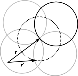
Figure 1: Set of hard spheres that are included in $n_{0}(\mathbf{r})$, which consist of those which just touch the point $\mathbf{r}$.

In contrast, the asymmetrically averaged $A$ correlation function is given by

$$g^{A}_{\sigma}(\textbf{r}) =\frac{1}{n(\textbf{r})n_{A}(\textbf{r})}\int n^{(2)}(\textbf{r},\textbf{r}+\textbf{r}^{\prime})\frac{\delta(\sigma-|\textbf{r}^{\prime}|)}{4\pi\sigma^{2}}d\textbf{r}^{\prime}$$ (4)

where the density $n_{A}(\textbf{r})$ is similar to $n_{0}$, but measures the density of spheres that are touching a sphere that is located at point r.

$$n_{A}(\textbf{r}) =\int n(\textbf{r}^{\prime})\frac{\delta(\sigma-|\textbf{r}-\textbf{r}^{\prime}|)}{4\pi\sigma^{2}}d\textbf{r}^{\prime}$$ (5)

Thus $g_{\sigma}^{A}$ corresponds to an average of the two-particle density over spheres touching a sphere that is located at the position r.

Fundamental-Measure Theory

We use the White Bear version of the Fundamental-Measure Theory (FMT) functional roth2002whitebear , which describes the excess free energy of a hard-sphere fluid. The White Bear functional reduces to the Carnahan-Starling equation of state for homogeneous systems. It is written as an integral over all space of a local function of a set of “fundamental measures” $n_{\alpha}(\textbf{r})$, each of which is written as a one-center convolution of the density. The White Bear free energy is thus

$$A_{\textit{HS}}[n]=k_{B}T\int\left(\Phi_{1}(\textbf{r})+\Phi_{2}(\textbf{r})+\Phi_{3}(\textbf{r})\right)d\textbf{r}\;,$$ (6)

with integrands

$$\Phi_{1} =-n_{0}\ln\left(1-n_{3}\right)$$ (7)

$$\Phi_{2} =\frac{n_{1}n_{2}-\mathbf{n}_{V1}\cdot\mathbf{n}_{V2}}{1-n_{3}}$$ (8)

$$\Phi_{3} =(n_{2}^{3}-3n_{2}\mathbf{n}_{V2}\cdot\mathbf{n}_{V2})\frac{n_{3}+(1-n_{3})^{2}\ln(1-n_{3})}{36\pi n_{3}^{2}\left(1-n_{3}\right)^{2}},$$ (9)

using the fundamental measures

$$n_{3}(\textbf{r}) =\int n(\textbf{r}^{\prime})\Theta(\sigma/2-\left|\textbf{r}-\textbf{r}^{\prime}\right|)d\textbf{r}^{\prime}$$ (10)

$$n_{2}(\textbf{r}) =\int n(\textbf{r}^{\prime})\delta(\sigma/2-\left|\textbf{r}-\textbf{r}^{\prime}\right|)d\textbf{r}^{\prime}$$ (11)

$$\mathbf{n}_{2V}(\textbf{r}) =\int n(\textbf{r}^{\prime})\delta(\sigma/2-\left|\textbf{r}-\textbf{r}^{\prime}\right|)\frac{\textbf{r}-\textbf{r}^{\prime}}{|\textbf{r}-\textbf{r}^{\prime}|}d\textbf{r}^{\prime}$$ (12)

$$\mathbf{n}_{V1}=\frac{\mathbf{n}_{V2}}{2\pi\sigma},\quad n_{1} =\frac{n_{2}}{2\pi\sigma},\quad n_{0}=\frac{n_{2}}{\pi\sigma^{2}}$$ (13)

III Theoretical Approaches

III.1 Homogeneous limit

In order to motivate our derivation of the correlation function at contact for the inhomogeneous hard-sphere fluid, we begin by deriving the well-known formula for $g_{\sigma}$ for the homogeneous fluid that comes from the Carnahan-Starling free energy. The contact value of the correlation function density can be found by using the contact-value theorem, which states that the pressure on any hard surface is determined by the density at contact:

$$p =k_{B}Tn_{\textit{contact}}$$ (14)

$$=k_{B}Tng_{\sigma}$$ (15)

Since we are interested in the correlation function at the surface of the hard spheres, we need to compute the pressure on that surface. The pressure on a hard sphere can be readily computed from the dependence of the Carnahan-Starling free energy on hard sphere radius.

$$A_{HS} =Nk_{B}T\frac{4\eta-3\eta^{2}}{(1-\eta)^{2}}$$ (16)

where $\eta\equiv\frac{\pi}{6}\sigma^{3}n$ is the filling fraction. We can thus readily compute the derivative of free energy with respect to hard-sphere diameter, which is half the force on all the hard spheres—since we’re changing all their diameters at once. To compute the pressure on the spheres, we need to divide the total force by the total area of contact, which means dividing by $N4\pi\sigma^{2}$.

$$p_{\sigma} =\frac{1}{N4\pi\sigma^{2}}\frac{1}{2}\frac{dA_{HS}}{d\sigma}$$ (17)

$$=k_{B}Tn\frac{1-\frac{\eta}{2}}{(1-\eta)^{3}}$$ (18)

Using the contact-value theorem, we can thus find the well-known correlation function evaluated at contact.

$$g_{\sigma} =\frac{1-\frac{\eta}{2}}{(1-\eta)^{3}}$$ (19)

Extending this derivation to the inhomogeneous fluid requires that we find the pressure felt by the surface of particular spheres.

III.2 Asymmetrically averaged correlation function

We will begin our derivation of the locally averaged correlation function with the asymmetric definition of $g_{\sigma}^{A}(\textbf{r})$ given in Equation 4, which is averaged over contacts in which one of the two spheres is located at position r. This correlation function is related to the contact density averaged over the surface of a sphere located at r, and can thus be determined by finding the pressure on that sphere. We find this pressure from the change in free energy resulting from an infinitesimal expansion of any spheres located at position r. From this pressure, we derive a formula for the correlation function $g_{\sigma}^{A}(\textbf{r})$ as was done in the previous section:

$$p_{\sigma}(\mathbf{r}) =\frac{1}{n(\textbf{r})2\pi\sigma^{2}}\frac{\delta A_{HS}}{\delta\sigma(\mathbf{r})}$$ (20)

$$g_{\sigma}^{A}(\textbf{r}) =\frac{1}{n(\textbf{r})n_{A}(\textbf{r})}\frac{1}{k_{B}T2\pi\sigma^{2}}\frac{\delta A_{HS}}{\delta\sigma(\mathbf{r})}$$ (21)

Details of evaluating the functional derivative in Equation 21 using FMT are given in the appendix. The equation for $g_{\sigma}^{A}$ requires finding convolutions of local derivatives of the free energy, making this formulation computationally somewhat more expensive than the free energy itself.

III.3 Symmetrically averaged correlation function

We now address the symmetrically averaged correlation function, which is defined in Equation 2. This corresponds to the correlation function averaged for spheres touching at a given point. In this case, we conceptually would like to evaluate the pressure felt by the surface of spheres where that surface is located at point r. We can approximate this value by assuming that this pressure will be simply related to the free energy density at point r. Through a process similar to the previous derivations, this leads to the expression

$$g_{\sigma}^{S}(\textbf{r}) =\frac{1}{n_{0}(\textbf{r})^{2}}\frac{1}{2\pi\sigma^{2}}\frac{\partial\Phi(\textbf{r})}{\partial\sigma}$$ (22)

where $\Phi(\textbf{r})=\Phi_{1}(\textbf{r})+\Phi_{2}(\textbf{r})+\Phi_{3}(\textbf{r})$ is the dimensionless free energy density. This step is an approximation—unlike the analogous Equation 21—because it assumes that we have available a local functional $\Phi(\textbf{r})$ whose derivative provides the pressure needed to compute $g_{\sigma}(\textbf{r})$. Equation 22 requires that we evaluate the derivatives of the fundamental measures $n_{\alpha}(\textbf{r})$ with respect to diameter, which leads us to derivatives of the $\delta$ function, which we can simplify and approximate using an assumption of a reasonably smooth density:

$$\frac{\partial n_{2}(\textbf{r})}{\partial\sigma} =\frac{1}{2}\int\delta^{\prime}(\frac{\sigma}{2}-|\textbf{r}-\textbf{r}^{\prime}|)n(\textbf{r}^{\prime})d\textbf{r}^{\prime}$$ (23)

$$=\frac{2}{\sigma}n_{2}(\textbf{r})-\frac{1}{2}\int\delta\left(\frac{\sigma}{2}-|\textbf{r}-\textbf{r}^{\prime}|\right)\frac{\textbf{r}-\textbf{r}^{\prime}}{|\textbf{r}-\textbf{r}^{\prime}|}\cdot\mathbf{\nabla}n(\textbf{r}^{\prime})d\textbf{r}^{\prime}$$ (24)

$$\approx\frac{2}{\sigma}n_{2}(\textbf{r})$$ (25)

In the systems that we study, the density is not reasonably smooth, but we can state empirically making this approximation nevertheless improves the predictions of our functional, while at the same time reducing its computational cost by avoiding the need to calculate any additional weighted densities or convolutions.

III.4 Gross’s asymmetrically averaged correlation functional

One approximation for the correlation function is that of Grossgross2009density , which is of the asymmetrically averaged variety ($g_{\sigma}^{A}$):

$$g_{\sigma}^{\text{Gross,A}}(\textbf{r}) =\frac{1-\frac{\pi}{12}\sigma^{3}n_{A}(\textbf{r})}{\left(1-\frac{\pi}{6}\sigma^{3}n_{A}(\textbf{r})\right)^{3}}$$ (26)

where $n_{A}$ is the averaged density defined in Equation 5. This formula is arrived at by using the density averaged over all spheres that could be touching a sphere at point r in the Carnahan-Starling equation for the correlation function at contact, given in Equation 19.

III.5 Yu and Wu’s symmetrically averaged functional

Yu and Wu developed a functional for the correlation function evaluated at contact which is symmetrically averaged yu2002fmt-dft-inhomogeneous-associating . However, instead of using $n_{0}$ as the corresponding density, they use a density given by

$$n_{\text{Yu}}(\textbf{r}) =n_{0}(\textbf{r})\zeta(\textbf{r})$$ (27)

$$\zeta =1-\frac{\mathbf{n_{2}}\cdot\mathbf{n_{2}}}{n_{2}^{2}}$$ (28)

where the function $\zeta$ is a measure of local inhomogeneity at the point of contact, and has the effect of reducing this density at interfaces. Because of this difference, the correlation function of Yu and Wu cannot be directly compared with $g_{\sigma}^{S}$ as defined in Equation 2. Therefore in order to make a comparison we move the factors of $\zeta$ in Equation 27 from the density into the correlation function itself.

$$g_{\sigma}^{\text{Yu,S}} =\zeta^{2}g_{\sigma}^{\text{Yu}}$$ (29)

$$=\zeta^{2}\left(\frac{1}{1-n_{3}}+\frac{1}{4}\frac{\sigma n_{2}\zeta}{(1-n_{3})^{2}}+\frac{1}{72}\frac{\sigma^{2}n_{2}^{2}\zeta}{(1-n_{3})^{3}}\right)$$ (30)

where $g_{\sigma}^{\text{Yu}}$ is the correlation function as defined in reference yu2002fmt-dft-inhomogeneous-associating , and $g_{\sigma}^{\text{Yu,S}}$ is the function we will examine in this paper.

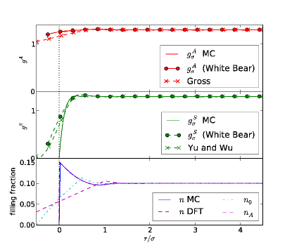
Figure 2: Density and correlation function at a hard wall with bulk filling fraction of 0.1.

IV Comparison with simulation

We performed a Monte-Carlo simulation of the hard sphere fluid to measure the contact value of the correlation function for several simple inhomogeneous configurations. For each configuration, we compute the mean density, and the contact values of the correlation function, averaged as defined in Equations 4 and 2. We compare these with the functionals presented in sections III.2 to III.5. We constructed our functionals using both the original White Bear functional roth2002whitebear as well as the mark II version of the White Bear functional hansen2006density , but the results were essentially indistinguishable on our plots, so we exclusively show the results due to the original White Bear functional.

We simulate the inhomogeneous hard sphere fluid at four hard-wall interfaces. The first and simplest is a flat hard wall. We then study two convex hard surfaces. One is an excluded sphere with diameter $2\sigma$, which corresponds to a “test particle” simulation with one of a hard sphere at the origin with diameter $\sigma$. The second is an excluded sphere with diameter $6\sigma$, which demonstrates behavior typical of mildly convex hard surfaces. Finally, we study a concave surface given by a hard cavity in which our fluid is free to move up to a diameter of $16\sigma$, which demonstrates behavior typical of mildly concave surfaces. In each case, we performed a low-density (filling fraction 0.1) and high-density (filling fraction 0.4) simulation. We performed additional computations over a wider range of curvatures and densities, but chose these as typical examples.

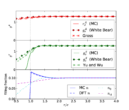
Figure 3: Density and correlation function around a hard sphere with diameter the same as those in the fluid, with a bulk filling fraction of 0.1.

IV.1 Low density

We begin by presenting our low-density results, corresponding to a filling fraction of 0.1, which are shown in Figures 2-5. At this low density, the contact value of the correlation function in the bulk is only 1.3, indicating that correlations are indeed small and that the fluid should be relatively easy to model. Indeed, the contact density at the hard surface is only around 50% higher than the bulk, and the FMT predicted density is close to indistinguishable from the true density for each of the four configurations.

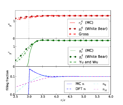
Figure 4: Density and correlation function around a hard sphere with an excluded diameter of $6\sigma$, with a bulk filling fraction of 0.1.

The $g_{\sigma}^{A}$ correlation function in each configuration is very flat, with only small, smooth changes as the surface is approached. Our functional $g_{\sigma}^{A}$ very closely matches the Monte Carlo predictions in each case, while that of Gross consistently underestimates the correlation at the interface by a significant margin. We note that the theoretical curves extend into the region from which the fluid is excluded. This value corresponds to the correlation function that would be observed in the vanishingly unlikely scenario in which there was a sphere present at that location. Naturally, we are unable to observe this quantity in our Monte Carlo simulations.

The $g_{\sigma}^{S}$ correlation function shows considerably more structure, as well as additional variation due to the curvature of the hard surface. The symmetric correlation function is nonzero at locations where spheres may touch, which for a convex hard surface means that $g_{\sigma}^{S}$ may be nonzero in the volume in which hard spheres are excluded. In every configuration studied, the agreement between the theoretical predictions and the Monte Carlo simulation in each case is very poor in the region where there should be no contacts at all. Because $n_{0}$ is comparable to its bulk value in this region, this means that these functionals predict a significant number of contacts in the region where there should be none. The correlation function of Yu and Wu yu2002fmt-dft-inhomogeneous-associating and ours described in Section III.3 give similar results, with slightly larger errors in our prediction.

Figure 5: Density and correlation functions near the surface of a spherical cavity with diameter $16\sigma$ at a bulk filling fraction of 0.1.

IV.2 High density

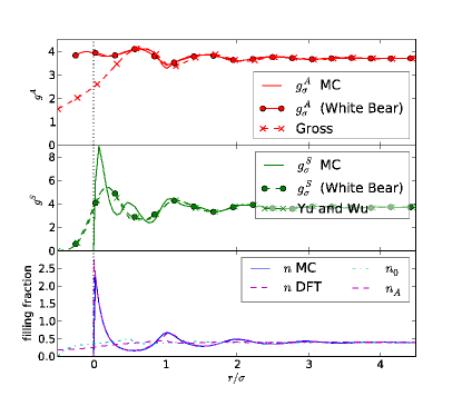
Figure 6: Density and correlation function at a hard wall with bulk filling fraction of 0.4.

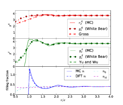
Figure 7: Density and correlation function around a hard sphere with diameter the same as those in the fluid, with a bulk filling fraction of 0.4.

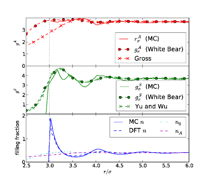
Figure 8: Density and correlation function around a hard sphere with an excluded diameter of $6\sigma$, with a bulk filling fraction of 0.4.

At a higher density corresponding to a filling fraction of 0.4, correlations are much stronger, with the bulk contact value of the correlation function of 3.7, as seen in Figures 6-9. This results in larger oscillations in the density at the hard surfaces, and correspondingly more interesting behavior in the correlation function near the interface. The density predicted by the White Bear functional agrees reasonably well with the simulation results, although not so well as it did at lower density. The discrepancies are largest in the case of the spherical cavity, in which the DFT considerably underestimates the range of the density oscillations.

The asymmetric version of the correlation function once again displays relatively smooth behavior with a few small oscillations near the interface, and a somewhat elevated value within a diameter of the hard surface, with the magnitude of this elevation somewhat different in each configuration. As was the case at low density, our correlation function $g_{\sigma}^{A}$ matches very closely the Monte Carlo data, reproducing quite well the structure near the interface in each configuration, although in the spherical cavity (Figure 9), there is a small, but significant discrepancy, comparable to the discrepancy found in the density itself. In each case, the correlation of Gross dramatically underestimates the correlation at the interface, at one extreme by 40% in the case of the spherical cavity (Figure 9), and at the other extreme by 15% in the test-particle scenario (Figure 7).

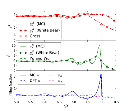
Figure 9: Density and correlation functions near the surface of a spherical cavity with diameter $16\sigma$ at a bulk filling fraction of 0.4.

The symmetrically averaged correlation function shows considerably more structure near the interface at high density, and this structure varies considerably depending on the curvature of the hard surface. In each case, this structure is not reflected in the theoretical predictions, neither that of this paper, nor that of Yu and Wu yu2002fmt-dft-inhomogeneous-associating . As was the case at low density, both functionals give significant and finite values in the region in which there are no contacts, but at high density they also miss the large oscillations that are present near the flat wall and the concave surface (Figures 6 and 9). As was the case at low density, the functional of Yu and Wu yu2002fmt-dft-inhomogeneous-associating gives slightly better agreement with the simulation results than that which we derive in Section III.3.

V Conclusion

We investigated several approximations to the contact value of the correlation function for inhomogeneous fluid distributions corresponding to flat, concave, and convex walls. We defined and simulated two averages of the correlation function, an asymmetric $A$ average centered at the location of one of the two spheres that is in contact, and a symmetric $S$ average centered at the point of contact of touching spheres. For each average, we derived a functional form from FMT, and also found an approximation that has been used in the literature. When compared with essentially exact Monte Carlo simulations, the $A$ correlation function derived from Fundamental Measure Theory in Section III.2 gives excellent results for each surface, at both high density and low density. The other three approximations that we studied all showed significant and systematic deviations under some circumstances. Thus, we recommend that creators of SAFT-based classical density functionals consider using the $g_{\sigma}^{A}$ functional defined in Section III.2.

Appendix

The expression for the asymmetric correlation function $g_{\sigma}^{A}(\textbf{r})$ (Equation 21) involves the functional derivative $\frac{\delta A_{HS}}{\delta\sigma(\mathbf{r})}$. In this appendix we will explain how this derivative is evaluated. We begin by applying the chain rule in the following way:

$$\frac{\delta A_{HS}}{\delta\sigma(\mathbf{r})} =\int\left(\sum_{\alpha}\frac{\delta A_{HS}}{\delta n_{\alpha}(\mathbf{r}^{\prime})}\frac{\delta n_{\alpha}(\mathbf{r}^{\prime})}{\delta\sigma(\mathbf{r})}\right)d\mathbf{r}^{\prime}$$ (31)

This expression requires us to evaluate $\frac{\delta A_{HS}}{\delta n_{\alpha}(\mathbf{r}^{\prime})}$ and $\frac{\delta n_{\alpha}(\mathbf{r}^{\prime})}{\delta\sigma(\mathbf{r})}$. The former is straightforward, given Equations 7-9, and we will write no more about it. The functional derivatives of the fundamental measures, however, require a bit more subtlety, and we will address them here.

We begin with the derivative of $n_{3}$, the filling fraction, which we will discuss in somewhat more detail than the remainder, which are similar in nature. Because the diameter $\sigma(\textbf{r})$ is the diameter of a sphere at position r, we write the fundamental measure $n_{3}(\textbf{r}^{\prime})$ as

$$n_{3}(\textbf{r}^{\prime}) =\int n(\textbf{r}^{\prime\prime})\Theta\left(\frac{\sigma(\textbf{r}^{\prime\prime})}{2}-\left|\textbf{r}^{\prime}-\textbf{r}^{\prime\prime}\right|\right)d\textbf{r}^{\prime\prime}$$ (32)

where we note that $\sigma(\textbf{r}^{\prime\prime})$ and $n(\textbf{r}^{\prime\prime})$ are the diameter and density, respectively, of spheres centered at position $\textbf{r}^{\prime\prime}$. Thus the derivative with respect to the diameter of spheres at position r is

$$\frac{\delta n_{3}(\textbf{r}^{\prime})}{\delta\sigma(\textbf{r})} =\frac{1}{2}\int n(\textbf{r}^{\prime\prime})\delta\left(\frac{\sigma(\textbf{r}^{\prime\prime})}{2}-\left|\textbf{r}^{\prime}-\textbf{r}^{\prime\prime}\right|\right)\delta(\textbf{r}-\textbf{r}^{\prime\prime})d\textbf{r}^{\prime\prime}$$ (33)

$$=n(\textbf{r})\delta(\sigma(\textbf{r})/2-\left|\textbf{r}^{\prime}-\textbf{r}\right|)$$ (34)

This pattern will hold for each fundamental measure: because we are seeking the change in free energy when spheres at point r are expanded, the integral over density is eliminated. To compute the correlation funtion $g_{\sigma}^{A}$, we convolve this delta function with the product of the density and a local derivative of $\Phi(\textbf{r})$:

$$\frac{\delta A_{HS}}{\delta\sigma(\textbf{r})} =\int\frac{\partial\Phi(\textbf{r}^{\prime})}{\partial n_{3}(\textbf{r}^{\prime})}n(\textbf{r}^{\prime})\delta(\sigma/2-|\textbf{r}^{\prime}-\textbf{r}|)d\textbf{r}^{\prime}+\cdots$$ (35)

As we shall see, there are only four convolution kernels, leading to four additional convolutions beyond those required for FMT.

The functional derivative of $n_{2}$ introduces our second convolution kernel, which is a derivative of the delta function.

$$\frac{\delta n_{2}(\textbf{r}^{\prime})}{\delta\sigma(\textbf{r})} =\frac{1}{2}n(\textbf{r})\delta^{\prime}(\sigma(\textbf{r})/2-\left|\textbf{r}^{\prime}-\textbf{r}\right|)$$ (36)

The derivatives of the remaining scalar densities $n_{1}$ and $n_{0}$ reduce to sums of the terms above:

$$\frac{\delta n_{1}(\textbf{r}^{\prime})}{\delta\sigma(\textbf{r})}=\frac{n(\textbf{r})}{4\pi\sigma(\textbf{r})}\delta^{\prime}(\sigma(\textbf{r})/2-\left|\textbf{r}^{\prime}-\textbf{r}\right|)\\ -\frac{n(\textbf{r})}{2\pi\sigma(\textbf{r})^{2}}\delta(\sigma(\textbf{r})/2-\left|\textbf{r}^{\prime}-\textbf{r}\right|)$$ (37)

and

$$\frac{\delta n_{0}(\textbf{r}^{\prime})}{\delta\sigma(\textbf{r})}=\frac{n(\textbf{r})}{2\pi\sigma(\textbf{r})^{2}}\delta^{\prime}(\sigma(\textbf{r})/2-\left|\textbf{r}^{\prime}-\textbf{r}\right|)\\ -2\frac{n(\textbf{r})}{\pi\sigma(\textbf{r})^{3}}\delta(\sigma(\textbf{r})/2-\left|\textbf{r}^{\prime}-\textbf{r}\right|)$$ (38)

The vector-weighted densities $\mathbf{n}_{V1}$ and $\mathbf{n}_{V2}$ give terms analogous to those of $n_{1}$ and $n_{2}$:

$$\frac{\delta\mathbf{n}_{V2}(\textbf{r}^{\prime})}{\delta\sigma(\textbf{r})}=-\frac{1}{2}n(\textbf{r})\delta^{\prime}(\sigma(\textbf{r})/2-\left|\textbf{r}^{\prime}-\textbf{r}\right|)\frac{\textbf{r}-\textbf{r}^{\prime}}{|\textbf{r}-\textbf{r}^{\prime}|}$$ (39)

$$\frac{\delta\mathbf{n}_{V1}(\textbf{r}^{\prime})}{\delta\sigma(\textbf{r})}=-\frac{n(\textbf{r})}{4\pi\sigma(\textbf{r})}\delta^{\prime}(\sigma(\textbf{r})/2-\left|\textbf{r}^{\prime}-\textbf{r}\right|)\frac{\textbf{r}-\textbf{r}^{\prime}}{|\textbf{r}-\textbf{r}^{\prime}|}\\ +\frac{n(\textbf{r})}{2\pi\sigma(\textbf{r})^{2}}\delta(\sigma(\textbf{r})/2-\left|\textbf{r}^{\prime}-\textbf{r}\right|)\frac{\textbf{r}-\textbf{r}^{\prime}}{|\textbf{r}-\textbf{r}^{\prime}|}$$ (40)

Thus there are four convolution kernels used in computing $g_{\sigma}^{A}$: one scalar and one vector delta function, and one scalar and one vector derivative of the delta function.

References

- (1) R. Roth, R. Evans, A. Lang, and G. Kahl, Journal of Physics: Condensed Matter 14, 12063 (2002).
- (2) Y. X. Yu and J. Wu, The Journal of Chemical Physics 116, 7094 (2002).
- (3) J. Gross, The Journal of chemical physics 131, 204705 (2009).
- (4) J. FELIPE, E. DEL RÍO, E. De Miguel, and G. Jackson, Molecular Physics 99, 1851 (2001).
- (5) G. Gloor, F. Blas, E. del Rio, E. de Miguel, and G. Jackson, Fluid phase equilibria 194, 521 (2002).
- (6) G. Gloor, G. Jackson, F. Blas, E. Del Río, and E. de Miguel, The Journal of chemical physics 121, 12740 (2004).
- (7) G. Clark, A. Haslam, A. Galindo, and G. Jackson, Molecular physics 104, 3561 (2006).
- (8) G. Gloor, G. Jackson, F. Blas, E. del Río, and E. de Miguel, The Journal of Physical Chemistry C 111, 15513 (2007).
- (9) H. Kahl and J. Winkelmann, Fluid Phase Equilibria 270, 50 (2008).
- (10) D. Fu and J. Wu, Ind. Eng. Chem. Res 44, 1120 (2005).
- (11) P. Bryk, S. Sokołowski, and O. Pizio, The Journal of chemical physics 125, 024909 (2006).
- (12) H. Hansen-Goos and R. Roth, Journal of Physics: Condensed Matter 18, 8413 (2006).