Comparison of Gamow-Teller strengths in the random phase approximation

Abstract

The Gamow-Teller response is astrophysically important for a number of nuclides, particularly around iron. The random phase approximation (RPA) is an efficient way to generate strength distributions. In order to better understand both theoretical systematics and uncertainties, we compare the Gamow-Teller strength distributions for a suite of nuclides and for a suite of interactions, including semi-realistic interactions in the $1p$-$0f$ space with the RPA and a separable multi-shell interaction in the quasi-particle RPA. We also compare with experimental results where available.

1 Introduction

Gamow-Teller (GT) electron capture ($\beta$-decay) transitions, caused by the $\sigma\tau_{+}$ ($\sigma\tau_{-}$) operator, are some of the most important nuclear weak processes in astrophysics. For a review of spin-isospin transitions see Ref. [1]. The GT transitions in $fp$-shell nuclei play important roles at the core collapse stages of supernovae, specially in neutrino induced processes. One of the factors controlling the gravitational core-collapse of massive stars is the lepton fraction; the lepton fraction in turn is governed by $\beta$-decay and electron capture rates among iron-regime nuclides. A primary and non-trivial contribution to the weak rates is the distribution of GT strength. GT strengths have important implications in other astrophysical scenarios as well, such as explosive nucleosynthesis in O-Ne-Mg white dwarfs (see Ref. [2] and references therein) .

GT distributions have been extracted experimentally using different techniques. Whereas the $\beta$-decay extraction is done in a model independent manner and are used to calibrate the B(GT), the charge-exchange reactions require further assumptions and the resulting extraction of GT distributions cannot be truly done in a model-independent manner. Consequently astrophysical calculations rely either upon crude estimates or upon more detailed microscopic calculations. The main difficulty with both experiment and theory is that the strength distribution connects to many states. Further in astrophysical environments one needs finite temperature GT strength functions as the temperature is high enough for excited states in the parent to be thermally populated.

The isovector response of nuclei may be studied using the nucleon charge-exchange reactions $(p,n)$ or $(n,p)$; by other reactions such as $(^{3}$He,$t$), ($d,^{2}$He) or through heavy ion reactions. The $0^{0}$ GT cross sections ($\Delta T=1,\Delta S=1,\Delta L=0,\hskip 2.84544pt0\hbar\omega$ excitations) are proportional to the analogous beta-decay strengths. Charge-exchange reactions at small momentum transfer can therefore be used to study beta-decay strength distributions when beta-decay is not energetically possible. The $(p,n)$, $(^{3}$He,$t)$ reactions probe the GT_- strength (corresponding to $\beta^{-}$-decay) and the $(n,p)$, $(d,^{2}$He) reactions give the strength for $\beta^{+}$-decay/electron capture, i.e. GT₊ strength. The study of $(p,n)$ reactions has the advantage over $\beta$-decay measurements in that the GT_- strength can be investigated over a large region of excitation energy in the residual nucleus. On the other hand the $(n,p)$ reactions populates only $T=T_{0}+1$ states in all nuclei heavier than ³He. This means that other final states (including the isobaric analog resonance) are forbidden and GT₊ transitions can be observed relatively free of background. The study of these reactions suggest that a reduction in the amount of GT strength is observed relative to theoretical calculations. The GT quenching is on the order of 30-40 $\%$ [3].

Theory for GT transitions falls generally into three camps: simple independent-particle models (e.g. Ref. [4]); full-scale interacting shell-model calculations; and, in between, the random-phase approximation (RPA) and quasi-particle random-phase approximation (QRPA). Independent-particle models underestimate the the total GT strength, because the Fermi surface is insufficiently fragmented, while also placing the centroid of the GT strength too high for even-even parent nuclides and too low on odd-A and odd-odd parents [5]. Full interacting shell-model calculations are computationally demanding, although one can exploit the Lanczos algorithm, commonly used in large shell-model diagonalization [6], to efficiently generate the strength distribution [7]; for medium-mass nuclei one still needs to choose from among a number of competing semi-realistic/semi-empirical interactions. RPA and QRPA can be thought of as approximations to a full shell-model calculation and are much less demanding computationally.

In this paper we compare GT strength distributions for a suite of iron-region nuclides relevant to astrophysics: ^54,55,56Fe, and ^56,58Ni. For each of these nuclides we compute the GT strengths in several RPA calculations. Each RPA calculation is in occupation rather than configuration space, which is appropriate inasmuch as the GT operator only affects spin and isospin. (In fact each calculation properly speaking is proton-neutron RPA or QRPA, as the RPA/QRPA phonon operators change protons into neutrons or vice-versa.) The calculations, which will be described in greater detail in subsequent sections, are :

$\bullet$ pn-RPA in a major harmonic oscillator shell, that is, the $1p$-$0f$ shell, with three different semi-realistic/semi-empirical interactions [8, 9, 10]. For details see Section 2.

$\bullet$ pn-QRPA in a multi-shell single-particle space with a schematic interaction that has been previously applied to similar calculations [11]. For further details we refer to Section 3.

These particular calculations were chosen because of the availability of codes; one could imagine a larger set of calculations (e.g., pn-QRPA with semi-realistic interactions) but relevant codes either do not exist or are not available to us.

These calculations will help to understand systematic similarities and differences between (a) different $1p$-$0f$ shell-model interactions and (b) between $0\hbar\Omega$ shell-model calculations against multi-shell calculations with a separable interaction. For example, for some cases in the $1s$-$0d$ shell the separable interactions yield a larger total strength and a higher centroid [12] than shell-model calculations.

Section 4 presents the results and discussions on use of various pn-RPA schemes. We finally present the summary and conclusions in Section 5.

2 The random phase approximation with shell-model interactions

The configuration-interaction (CI) shell model solves the many-body problem in a large basis of Slater determinants using the occupation representation. One advantage of the CI shell model is that it can use arbitrary two-body (or even higher-order) interactions and gives explicit wavefunctions for excited states as well as the ground state. In addition, because the GT operator is $\sigma\tau$ and does not affect coordinate space wavefunctions, the CI shell model is well suited for GT transitions. The drawback of the CI shell model is that even with including just a few, or even one, harmonic oscillator shell, the basis dimensions can be huge ($10^{9}$ or greater), making such calculations computationally intensive. Furthermore, limiting calculations to a few shells leads to the necessity for quenching (in the case of Gamow-Teller transitions) or enhancement (for example, E2 transitions) of coupling parameters.

The Hamiltonian for the shell-model is written in occupation space[13, 14, 7], i.e.,

$$\hat{H}=\sum_{a}\epsilon_{a}\hat{n}_{a}+\frac{1}{4}\sum_{abcd}V_{abcd}\hat{c}^{\dagger}_{a}\hat{c}^{\dagger}_{b}\hat{c}_{c}\hat{c}_{d}$$ (1)

where the creation and annihilation operators $\hat{c}_{a}^{\dagger},\hat{c}_{a}$ represent single-particle states with good angular momentum, and where $\epsilon_{a}$ are the single particle energies and $V_{abcd}$ are the two-body matrix elements.

It is possible to solve the RPA matrix equation in a shell-model representation, using the single-particle energies and two-body matrix elements above. A recent series of papers showed that RPA is a reasonable, if not perfect, approximation to the numerically exact results, comparing ground state correlation energies [15] and charge-conserving [16] and charge-changing [17] transitions; in the last case it was found that allowing the Hartree-Fock state to be deformed improved pn-RPA calculations of GT strength distributions.

The first step is a Hartree-Fock calculation, which introduces a unitary transformation on the single-particle states,

$$\hat{d}^{\dagger}_{\alpha}=\sum_{a}D_{\alpha a}\hat{c}^{\dagger}_{a}$$ (2)

These states are divided into occupied (hole) states, labeled by $m$, and unoccupied (particle) states labeled by $i$, and the transformation matrix $\mathbf{D}$ is chosen such that the energy of the Slater determinant $|\mathrm{HF}\rangle=\prod_{m}\hat{d}^{\dagger}_{m}|0\rangle$ minimizes the energy $\langle\mathrm{HF}|\hat{H}|\mathrm{HF}\rangle$.

With the Hartree-Fock solution in hand, one finds excited states (and the correlation energy in the ground state, although that does not concern us here) by treating the energy surface in the vicinity of the Hartree-Fock state as quadratic. This leads to the RPA matrix equations [13]. For charge-changing interactions such as Gamow-Teller, the RPA matrix equations take the form:

$$\left(\begin{array}[]{cccc}A^{np,pn}&0&0&B^{np,pn}\\ 0&A^{pn,np}&B^{pn,np}&0\\ 0&-B^{np,pn}&-A^{np,pn}&0\\ -B^{pn,np}&0&0&-A^{pn,np}\end{array}\right)\left(\begin{array}[]{c}X(pn)\\ X(np)\\ Y(np)\\ Y(pn)\end{array}\right)=\Omega\left(\begin{array}[]{c}X(pn)\\ X(np)\\ Y(np)\\ Y(pn)\end{array}\right),$$ (3)

where the definitions for $A^{pn,np}$ and $B^{np,pn}$ matrices are similar to the regular proton-neutron conserving formalism, where one approximates $|\mathrm{RPA}\rangle\approx|\mathrm{HF}\rangle$:

$$A_{mi,nj}^{np,pn}=\langle{\rm HF}|[\nu_{i}^{\dagger}\pi_{m},[H,\pi_{n}^{\dagger}\nu_{j}]]|{\rm HF}\rangle=(\epsilon^{p}_{n}-\epsilon_{i}^{n})\delta_{mn}\delta_{ij}-V^{pn}_{mn,ji},$$ (4)

$$B_{mi,nj}^{np,pn}=-\langle{\rm HF}|[\nu_{m}^{\dagger}\pi_{i},[\pi_{n}^{\dagger}\nu_{j},H]]|{\rm HF}\rangle=-V_{in,jm}^{pn}.$$ (5)

The matrices $A^{pn,np}$ and $B^{pn,np}$ are defined similarly, but are distinct unless $Z=N$; in fact, they have different dimensions unless $Z=N$. Let $N_{p}^{\pi}$, $N_{h}^{\pi}$ be number of proton particle and hole states, respectively, and $N_{p}^{\nu}$, $N_{h}^{\nu}$ the number of neutron particle and hole states. Thus the vectors $X(pn)$ and $Y(np)$ are of length $N_{p}^{\pi}N_{h}^{\nu}$ while vectors $X(np)$, $Y(pn)$ are of length $N_{p}^{\nu}N_{h}^{\pi}$; the two lengths are unequal unless $Z=N$. Similarly, $\mathbf{A}^{np,pn}$ is a square matrix of dimension $N_{p}^{\pi}N_{h}^{\nu}$ while $\mathbf{A}^{pn,np}$ is a square matrix of dimension $N_{p}^{\nu}N_{h}^{\pi}$, while $\mathbf{B}^{np,pn}$ is a rectangular matrix of dimension $N_{p}^{\pi}N_{h}^{\nu}\times N_{p}^{\nu}N_{h}^{\pi}$, and $\mathbf{B}^{pn,np}=\left(\mathbf{B}^{np,pn}\right)^{T}$ .

The transition strength is given by

$$\langle\mathrm{RPA}|{\cal O}|\lambda_{(Z\pm 1,N\mp 1)}\rangle=\langle\mathrm{RPA}|[{\cal O},\beta_{\lambda}^{\dagger}]|\mathrm{RPA}\rangle$$

$$=\sum_{mi}\left(X_{mi}^{\lambda}(pn/np){\cal O}_{mi}+Y_{mi}^{\lambda}(pn/np){\cal O}_{im}\right),$$ (6)

where $\beta_{\lambda}^{\dagger}$ is the transition operator for a $\beta$-decay, in this case the Gamow-Teller operator $\vec{\sigma}\tau_{\pm}$. For more details consult [17].

For this paper we use three different semi-realistic/semi-empirical shell model interactions. All three interactions started from realistic nucleon-nucleon interactions, from which an effective interaction (e.g., a G-matrix) was derived. At this point the interaction is expressed numerically as two-body matrix elements $V_{JT}(ab,cd)$. The interactions were all then further modified in order to fit experimental spectra; as is well-known to the shell-model community, most of the modification were to the “monopole” parts of the interaction, which are related to properties of the mean-field. All three interactions are similar, but have different starting points and were fitted to different data sets, with the following semi-realistic/semi-empirical interactions: the modified Kuo-Brown interaction KB3G [8] and the Brown-Richter interaction interaction FPD6G [9] and the Tokyo interaction GXPF1 [10]; the names do not signify much except that PF/FP refer to the $fp$ shell.

3 The quasi-particle random phase approximation with a separable interaction

For an alternate approach, we used the quasi-particle proton-neutron random phase approximation ($pn$-QRPA) with a separable interaction of the form

$$\hat{H}^{QRPA}=\hat{H}^{sp}+\hat{V}^{pair}+\hat{V}_{GT}^{ph}+\hat{V}_{GT}^{pp}$$ (7)

where $\hat{H}^{sp}$ is the single-particle Hamiltonian, $\hat{V}^{pair}$ is the pairing force, $\hat{V}^{ph}_{GT}$ and $\hat{V}^{pp}_{GT}$ are the particle-hole (ph) and particle-particle (pp) components, respectively, of the GT force $(\vec{\sigma}\vec{\tau})^{2}$. We diagonalized our Hamiltonian in three consecutive steps as outlined below.

Single-particle energies and wave functions were calculated in the Nilsson model which takes into account nuclear deformation [18]. The transformation from the spherical basis to the axial-symmetric deformed basis can be written as [11]

$$\hat{d}^{\dagger}_{m\alpha}=\sum_{j}D^{m\alpha}_{j}\hat{c}^{\dagger}_{jm},$$ (8)

where $\hat{d}^{\dagger}$ and $\hat{c}^{\dagger}$ are particle creation operators in the deformed and spherical basis, respectively; the transformation matrices $D^{m\alpha}_{j}$ were determined by diagonalization of the Nilsson Hamiltonian, and $\alpha$ represents additional quantum numbers, except $m$, which specify the Nilsson eigenstates.

Pairing was treated in the BCS approximation, where a constant pairing force with the force strength $G$ ($G_{p}$ and $G_{n}$ for protons and neutrons, respectively) was applied,

$$\hat{V}^{pair}=-G\sum_{jmj^{\prime}m^{\prime}}(-1)^{l+j-m}\hat{c}^{\dagger}_{jm}\hat{c}^{\dagger}_{j-m}(-1)^{l^{\prime}+j^{\prime}-m^{\prime}}\hat{c}_{j^{\prime}-m^{\prime}}\hat{c}_{j^{\prime}m^{\prime}},$$ (9)

where the sum over $m$ and $m^{\prime}$ was restricted to $m,m^{\prime}>0$, and $l$ represents the orbital angular momentum.

The BCS calculation gave the quasi-particle energies $\epsilon_{m\alpha}$. A quasi-particle basis was introduced via

$$\hat{a}^{\dagger}_{m\alpha}=u_{m\alpha}\hat{d}^{\dagger}_{m\alpha}-v_{m\alpha}\hat{d}_{\overline{m}\alpha},$$ (10)

$$\hat{a}^{\dagger}_{\overline{m}\alpha}=u_{m\alpha}\hat{d}^{\dagger}_{\overline{m}\alpha}+v_{m\alpha}\hat{d}_{m\alpha},$$ (11)

where $\overline{m}$ is the time-reversed state of $m$, and $\hat{a}^{\dagger}(\hat{a})$ are the quasi-particle creation (annihilation) operators which enter the RPA equation. The occupation amplitudes $u$ and $v$ satisfy the condition $u^{2}+v^{2}=1$ and were determined by the BCS equations (see for example [13], page 230).

In the pn-QRPA, charge-changing transitions are expressed in terms of phonon creation, with the QRPA phonons defined by

$$\hat{b}^{\dagger}_{\omega}(\mu)=\sum_{pn}(X^{pn}_{\omega}(\mu)\hat{a}^{\dagger}_{p}\hat{a}^{\dagger}_{\overline{n}}-Y^{pn}_{\omega}(\mu)\hat{a}_{n}\hat{a}_{\overline{p}}).$$ (12)

The sum in Eq. (12) runs over all proton-neutron pairs with $\mu=m_{p}-m_{n}=$ -1, 0, 1, where $m_{p(n)}$ denotes the third component of the angular momentum. The ground state of the theory is defined as the vacuum with respect to the QRPA phonons, $\hat{b}_{\omega}(\mu)|QRPA>=0$. The forward- and backward-going amplitudes $X$ and $Y$ are eigenfunctions of the RPA matrix equation

$$\left[\begin{array}[]{cc}A&B\\ -B&A\end{array}\right]\left[\begin{array}[]{c}X\\ Y\end{array}\right]=\omega\left[\begin{array}[]{c}X\\ Y\end{array}\right],$$ (13)

where $\omega$ are energy eigenvalues of the eigenstates and elements of the two submatrices are given by

$$A_{pn,p^{\prime}n^{\prime}} = \delta(pn,p^{\prime}n^{\prime})(\epsilon_{p}+\epsilon_{n})+V^{pp}_{pn,p^{\prime}n^{\prime}}(u_{p}u_{n}u_{p^{\prime}}u_{n^{\prime}}+v_{p}v_{n}v_{p^{\prime}}v_{n^{\prime}})+$$ (14)

$$V^{ph}_{pn^{\prime},p^{\prime}n^{\prime}}(u_{p}v_{n}u_{p^{\prime}}v_{n^{\prime}}+v_{p}u_{n}v_{p^{\prime}}u_{n^{\prime}}),$$

$$B_{pn,p^{\prime}n^{\prime}}=V^{pp}_{pn,p^{\prime}n^{\prime}}(u_{p}u_{n}v_{p^{\prime}}v_{n^{\prime}}+v_{p}v_{n}u_{p^{\prime}}u_{n^{\prime}})-V^{ph}_{pn,p^{\prime}n^{\prime}}(u_{p}v_{n}v_{p^{\prime}}u_{n^{\prime}}+v_{p}u_{n}u_{p^{\prime}}v_{n^{\prime}}).$$ (15)

The backward-going amplitude $Y$ accounts for the ground-state correlations. It is essential to note however, that the derivation of the QRPA matrix requires ground-state correlations to be only a small correction. It should be noted that $|Y|\ll|X|$ does not imply that ground-state correlations are negligible, since for the calculation of $\beta$ transition matrix elements one always must consider products of the form $uvY$ and $u^{\prime}v^{\prime}X$. Especially in $\beta^{+}$ decay, $uv$ can be larger than $u^{\prime}v^{\prime}$; thus ground-state correlations cannot be neglected. The RPA equation is constructed and solved for each value of the projection $\mu$, i.e., $\mu=$ -1, 0 and +1. The equation gives identical eigenvalue spectra for $\mu=$ -1 and $\mu=$ +1, and eigenvalues for $\mu=$ 0 are always two-fold degenerate, because of the axial symmetry of the Nilsson potential. (Hereafter, $\mu$ will be suppressed if not otherwise stated, since the following formulas hold for each $\mu$).

In the pn-QRPA formalism proton-neutron residual interactions occur in two different forms, namely as particle-hole (ph) and particle-particle (pp) interaction. Both the particle-hole and particle-particle interaction can be given a separable form.

In the present work, in addition to the well known particle-hole force [19, 20]

$$\hat{V}^{ph}_{GT}=2\chi\sum_{\mu}(-1)^{\mu}\hat{Y}_{\mu}\hat{Y}^{\dagger}_{-\mu},$$ (16)

with

$$\hat{Y}_{\mu}=\sum_{j_{p}m_{p}j_{n}m_{n}}\langle j_{p}m_{p}|t_{-}\sigma_{\mu}|j_{n}m_{n}\rangle\hat{c}^{\dagger}_{j_{p}m_{p}}\hat{c}_{j_{n}m_{n}},$$ (17)

the particle-particle interaction, approximated by the separable force [21, 22]

$$\hat{V}^{pp}_{GT}=-2\kappa\sum_{\mu}(-1)^{\mu}\hat{P}_{\mu}^{\dagger}\hat{P}_{-\mu},$$ (18)

with

$$\hat{P}^{\dagger}_{\mu}=\sum_{j_{p}m_{p}j_{n}m_{n}}\langle j_{n}m_{n}|(t_{-}\sigma_{\mu})^{+}|j_{p}m_{p}\rangle(-1)^{l_{n}+j_{n}-m_{n}}\hat{c}^{\dagger}_{j_{p}m_{p}}\hat{c}^{\dagger}_{j_{n}-m_{n}},$$ (19)

was taken into account. The interaction constants $\chi$ and $\kappa$ in units of MeV were both taken to be positive. The different signs of $V^{pp}$ and $V^{ph}$ reflect a well-known feature of the nucleon-nucleon interaction; namely, that the ph force is repulsive while the pp force is attractive. Instead of using a parametrization of chi and kappa values as a function of nucleon number, we chose to fix specific values of chi and kappa for each isotopic chain. Example giving in previous pn-QRPA calculation Homma and collaborators took $\chi=5.2/A^{0.7}$ MeV and $\kappa=0.58/A^{0.7}$ MeV [23]. These values were deduced from a fit to experimental half-lives and for every isotopic chain fixed values of chi and kappa allowed to deduce a locally best value of chi and kappa (see also Ref. [24] which uses the same recipe). For further study of effect of interaction constants, $\chi$ and $\kappa$, on the pn-QRPA calculations, we refer to [24, 25]. It was later shown that fixing values of $\chi$ and $\kappa$ for an isotopic chain led to better reproduction of experimental data [26, 27]. For the case of nickel and iron isotopes the values of interaction constants were taken accordingly from Ref. [26] and Ref. [27], respectively. The values of $\chi$ and $\kappa$, along with the value of deformation parameter, used in the current work, are shown in Table 1.

Using a separable interaction allows the pn-QRPA calculations to be solved in a much larger single-particle basis than with a general/semi-realistic interaction; in this case we used up to 7 $\hbar\omega$ shells. Such calculations have been used extensively in computing GT transitions for astrophysical applications for a wide variety of nuclide (e.g. [26, 28, 29, 30])

Matrix elements of the forces which appear in RPA equation (14),(15) are separable,

$$V^{ph}_{pn,p^{\prime}n^{\prime}}=+2\chi f_{pn}(\mu)f_{p^{\prime}n^{\prime}}(\mu),$$ (20)

$$V^{pp}_{pn,p^{\prime}n^{\prime}}=-2\kappa f_{pn}(\mu)f_{p^{\prime}n^{\prime}}(\mu),$$ (21)

with

$$f_{pn}(\mu)=\sum_{j_{p}j_{n}}D^{m_{p}\alpha_{p}}_{j_{p}}D^{m_{n}\alpha_{n}}_{j_{n}}\langle j_{p}m_{p}|t_{-}\sigma_{\mu}|j_{n}m_{n}\rangle,$$ (22)

which are single-particle GT transition amplitudes defined in the Nilsson basis. For the case of separable forces, the matrix equation (13) reduces to an algebraic equation of second order (when $\kappa$ = 0) and with a finite value of $\kappa$ it transforms to a fourth order equation. Methods of finding roots of these equations can be seen in Ref. [11]. For details on QRPA model parameters we refer to [26].

The purpose of this paper is to compare general trends of these calculations with the $0\hbar\omega$ calculations using a more general, realistic interaction described in the previous section.

4 Results and comparison

Using the Gamow-Teller operator $\vec{\sigma}\tau_{\pm}$ yields the Ikeda sum rule [31] for a parent nucleus with $Z$ protons and $N$ neutrons:

$$\sum B(GT_{-})-\sum B(GT_{+})=3(N-Z),$$ (23)

in our calculations. For use in astrophysical reaction rates, and to compare to experimental data, and to prior calculations, we multiply our results by a quenching factor of 0.6 [3] typical for nuclei. Note that we do not include the axial weak coupling constant $g_{A}$ as the published data and calculations we compare to also leave it out, see for example Eq. 1 in [37], which uses a quenching factor of $(0.74)^{2}=0.55$.

The ultimate goal is to provide reliable weak rates for astrophysical environments, many of which cannot be measured experimentally. Even theoretically this is a complex and difficult issue. For example, $\beta$-decay and capture rates are exponentially sensitive to the location of GT₊ resonance while the total GT strength affect the stellar rates in a more or less linear fashion [32]. In sufficiently hot astrophysical environments one must include rates with an excited parent state. But rates off excited states are difficult to get: an $(n,p)$ experiment on a nucleus $(Z,A)$ shows where in $(Z-1,A)$ the GT₊ centroid corresponding only to the ground state of $(Z,A)$ resides. The calculations described in this paper are also limited only to ground state parents, although we hope to tackle excited parents in the future. For a discussion of calculation of excited state GT strength functions we refer to [33] using the shell model and [34] using the pn-QRPA model.

For this paper we focus on the variation in Gamow-Teller strengths from different RPA calculations, to give us an idea of the theoretical uncertainty.

Table 2 shows the mutual comparison of the various RPA models used in this project. This table shows the values of the centroids, widths and total strength values of the calculated and measured (where available) GT distributions, both in $\beta^{-}$ and electron capture directions, for various iron-regime nuclei. It is clear from Table 2 that the GXPF1 interaction calculates the biggest value of the total GT strength. On the other end the pn-QRPA tends to calculate lower total strength values. Regarding the calculation of centroids in various RPA models, we note that the pn-QRPA calculated centroid resides at lower energy in daughter, except for the case of ⁵⁵Fe where the KB3G interaction calculates the lowest centroids in the electron capture direction. On the other extreme the GXPF1 calculates the highest centroids except for the case of ⁵⁵Fe where the pn-QRPA model tops the chart in the electron capture direction. One also notes that the pn-QRPA calculated GT strength distributions tend to have a larger width. For related discussion on the pn-QRPA built on a deformed self-consistent mean field basis obtained from two-body density-dependent Skyrme forces for iron mass region we refer to [35]. The calculated GT strength distributions using different interactions will next be discussed below.

An obvious question would be how the various RPA calculations compare with the measured data as well as full shell-model diagonalization. Thus we also show in Table 2 how the values of calculated GT centroids and total GT strengths (both in $\beta^{-}$ and electron capture directions), using various RPA models, compare with the available experimental data. For the sake of comparison we also include the shell model calculation using the GXPF1J Hamiltonian [36] taken from Table I of Ref. [37] (the centroid value was not available). The authors claimed that the GXPF1J interaction leads to spreading of calculated strength and better reproduction of observed strength in Fe and Ni isotopes (see also Ref. [38]). Overall, the differences between the shell-model diagonalization strengths and those from RPA calculations using shell-model interactions is similar to that previously reported [17]. The experimental centroids and widths were calculated from the reported measured data and all measured data are given to one decimal place in Table 2. For the $\beta^{-}$ side the measured data for ⁵⁴Fe were taken from Refs. [39, 3, 40, 41]. It is to be noted that the recent high-resolution (³He, $t$) charge-exchange reaction on ⁵⁴Fe performed by Adachi and collaborators [41] report a much lower value of $\sum B(GT_{-})$ = 4.00 $\pm$ 0.37 up to 12 MeV in ⁵⁴Co. Ref. [39] reported the total strength of $\sum B(GT_{-})$ = 7.8 $\pm$ 1.9 and was not able to calculate B(GT) values at discrete excitation energies beyond 4.5 MeV in daughter. Hence it was not possible for us to calculate the centroid and width in this particular case. For the electron capture direction, experimental data for ⁵⁴Fe were taken from Refs. [3, 42] as also mentioned in Table 2. Measured data for ⁵⁶Fe in the electron capture direction were taken from Refs. [42, 43] while for the $\beta^{-}$ direction we only quote the reported value of $\sum B(GT_{-})$ = 9.9 $\pm$ 2.4 by Rapaport and collaborators [39]. The authors were unable to extract GT strengths for discrete excited states beyond 5.9 MeV in ⁵⁶Co making it impossible for us to calculate the centroid and width in this case.

Recently $(p,n)$ charge-exchange reaction in inverse kinematics at intermediate energies were used to extract GT strengths for the unstable nucleus ⁵⁶Ni [44]. The authors reported a value of $\sum B(GT_{-})$ = 3.5 $\pm$ 0.3 and due an additional uncertainty in GT unit cross section (normalization factor of B(GT)) also quoted a value of $\sum B(GT_{-})$ = 3.8 $\pm$ 0.2 in Ref. [45]. For the case of ⁵⁸Ni, measured data were taken from Refs. [43, 46] for the electron capture direction. Along the $\beta^{-}$ direction, authors in Ref. [39] quoted the total strength of $\sum B(GT_{-})$ = 7.5 $\pm$ 1.8 and were unable to extract GT strengths for discrete excited states beyond 6.4 MeV in ⁵⁸Cu (accordingly we were unable to calculate centroid and width for this case in Table 2). Fujita and collaborators extracted GT strength using the (³He,t) reaction up to 8.3 MeV in ⁵⁸Cu [47] and later up to higher daughter energies of 13 MeV [48].

It is to be noted that we used a quenching factor of 0.6 for the calculated GT strength using the pn-QRPA model [27] which is normally done in stellar weak rate calculations and also discussed in Section 1. Note that the shell model interactions [37] calculated strengths were quenched by a universal quenching factor of 0.55 rather than 0.6. Table 2 shows that the pn-QRPA model calculates the centroid at a much lower energy than other shell model interactions. Further in all cases it is seen that the pn-QRPA model best reproduces the placement of measured centroid. The comparison is exceptionally good for the case of GT_- centroid of ⁵⁴Fe and for the GT₊ centroids of ⁵⁶Fe and ⁵⁸Ni. On the other hand the GXPF1 interaction calculates the highest centroid in daughter nuclei. The shell model interactions calculate much better total strengths in comparison with measured values. One should also keep in mind the uncertainties present in measurements where various energy cutoffs are used as a reasonable upper limit on the energy at which GT strength could be reliably related to measured $\Delta L=0$ cross-sections as well as slightly different values of quenching factor used in pn-QRPA and shell model interactions before comparing the calculated numbers with experimental data. The Ikeda sum rule is satisfied as seen in previous RPA calculations [17].

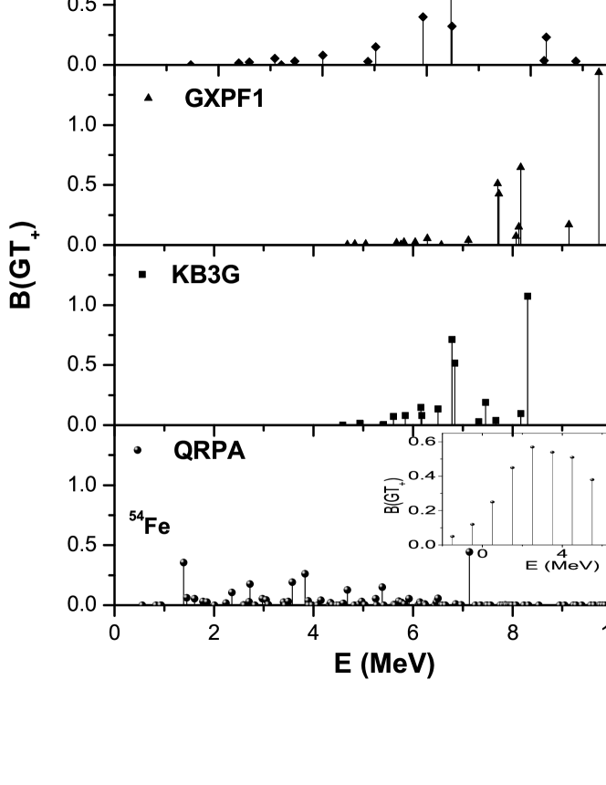
Figure 1: Calculated GT strength distributions in the electron capture direction for ⁵⁴Fe using different pn-RPA scenarios. For details of interactions used see text. In inset measured data of Ref. [42] is shown. The abscissa represents energy in daughter.

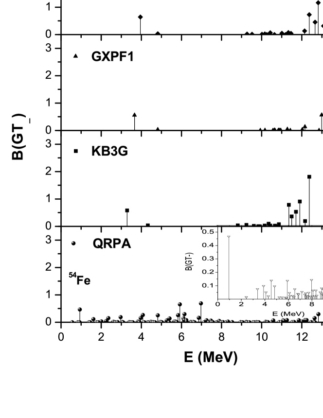
Figure 2: Same as in Fig. 1 but for calculated GT strength distributions in the $\beta^{-}$-decay direction. In inset the recent measured data of Ref. [41] is shown.

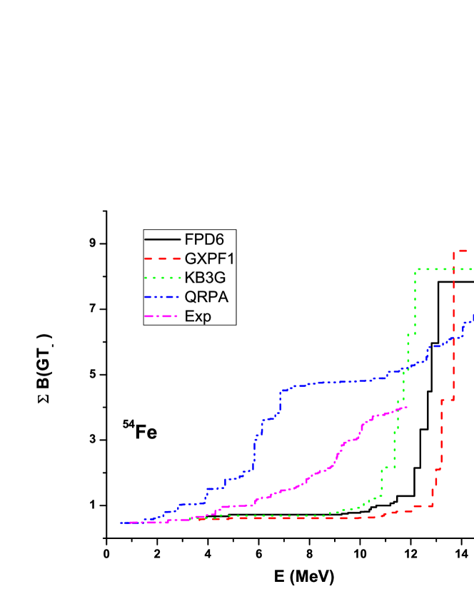
Figure 3: Cumulative GT strength distributions for ⁵⁴Fe using different pn-RPA scenarios in the $\beta^{-}$-decay direction. For details of interactions used see text. Experimental data (Exp) is taken from Ref. [41]. The abscissa represents energy in daughter.

Fig. 1 and Fig. 2 show the calculated GT strength distribution of ⁵⁴Fe in various RPA calculations. Fig. 1 displays the calculated GT strength distribution in the electron capture direction whereas Fig. 2 shows similar calculation in the $\beta^{-}$ direction. In the inset of Fig. 1 we also show the ⁵⁴Fe(n,p) reaction, measured at 97 MeV for excitation energies in ⁵⁴Mn [42]. Similarly we also show the recently measured high-resolution (³He, $t$) data on ⁵⁴Fe by Adachi and collaborators [41] in the inset of Fig. 2. Fig. 3 shows the cumulative strength distributions, in the $\beta^{-}$ direction, for various RPA calculations and measured data [41]. Fig. 3 depicts the mutual comparison of various calculations with measured data in a better fashion. It is noted that the pn-QRPA model calculates GT transitions at low excitation energy. It is further noted that the QRPA calculated distribution is better fragmented than other RPA models and follows the trend of the measured data, albeit with a much higher magnitude of strength distribution.

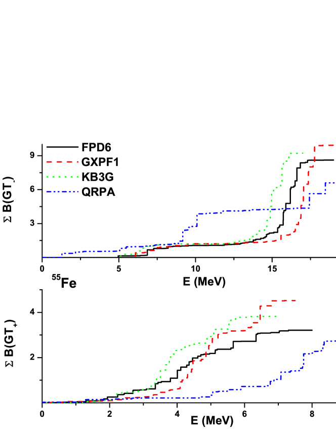
Figure 4: Cumulative GT strength distributions for ⁵⁵Fe using different pn-RPA scenarios. For details of interactions used see text. The abscissa represents energy in daughter.

For the remaining cases we decided to show only the cumulative GT strength distributions to save space. Fig. 4 display the cumulative strength distributions in a two-panel frame. The upper panel shows the cumulative strength distribution in the $\beta^{-}$ direction using the different RPA models whereas the lower panel displays the results in the electron capture direction for the case of ⁵⁵Fe. The pn-QRPA calculates high-lying transitions in ⁵⁵Co (upper panel). The KB3G interaction saturates first to its maximum strength in both directions and gives the lowest values for the centroid of the GT₊ distribution function. No measured GT strength of ⁵⁵Fe was available in literature to compare with the different calculations.

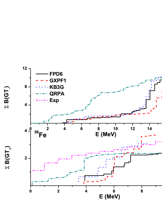
Figure 5: Cumulative GT strength distributions for ⁵⁶Fe using different pn-RPA scenarios. For details of interactions used see text. Experimental data (Exp) is taken from Ref. [43]. The abscissa represents energy in daughter.

A similar comparison of cumulative strength functions for the case of ⁵⁶Fe is shown in Fig. 5. Here we note that for the $\beta^{-}$ direction the measured GT strength distribution quote the value of $\sum B(GT_{-})$ = 9.9 $\pm$ 2.4 up to 15 MeV in daughter but extracts the B(GT) only up to discrete daughter excited states of 3.5 MeV [39]. Accordingly it was not possible for us to show the measured data in upper panel of Fig. 5. In the lower panel the measured data of Ref. [43] is shown for the electron capture direction of ⁵⁶Fe. Fig. 5 reveals that the pn-QRPA model peaks at a faster pace compared to other RPA models. Correspondingly the pn-QRPA calculates the lowest values for the centroids in both directions for ⁵⁶Fe (see Table 2). For the electron capture direction (lower panel) the pn-QRPA best mimics the trend in the measured GT data. It can be seen that the GT strength resides at much higher energies in the daughter nuclei in the $\beta^{-}$ direction for all models.

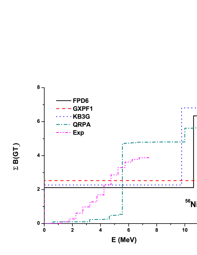
Figure 6: Cumulative GT strength distributions for the $N=Z$ nucleus ⁵⁶Ni using different pn-RPA scenarios in the $\beta^{-}$-decay direction. For details of interactions used see text. Experimental data (Exp) is taken from Ref. [45]. The abscissa represents energy in daughter.

Fig. 6 shows the GT strength distribution of $N=Z$ nucleus ⁵⁶Ni. Experimental data were taken from Ref. [45]. Here one notes that for the models used, all strength resides at one energy level in daughter nucleus for the FPD6, GXPF1 and KB3G interactions. This energy is 10.6, 11.5 and 9.8 MeV for the FPD6, GXPF1 and KB3G interactions, respectively. The recent shell model calculation by Suzuki et al. [37], using the GXPF1J interaction, showed that the GT strength distribution in ⁵⁶Ni is more fragmented and different from previous shell model calculations resulting in enhanced production yields of heavy elements. The authors further commented that the calculated GT strength using the GXPF1J interaction was found to be more fragmented with a remaining tail in the high excitation energy compared with that obtained by the KB3G interaction. For the case of ⁵⁶Ni their calculated strength was fragmented into two peaks whereas the total calculated strength was 11.32 (unquenched). On the other hand we note from Fig. 6 that the pn-QRPA calculated strength is still more fragmented over a range of energies with two distinct peaks at 5.7 MeV and 10.6 MeV in the daughter nucleus. The consequences of calculating a much more fragmented strength distribution for ⁵⁶Ni, using the pn-QRPA model, may also have interesting scenario for heavy element nucleosynthesis and requires further attention in nuclear network calculations.

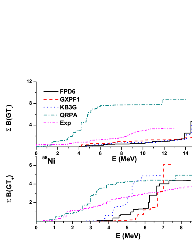
Figure 7: Cumulative GT strength distributions for ⁵⁸Ni using different pn-RPA scenarios. For details of interactions used see text. Experimental data (Exp) is taken from Ref. [47, 48] for the $\beta^{-}$-decay direction and from Ref. [46] for the electron capture direction. The abscissa represents energy in daughter.

The cumulative strength distributions for the case of ⁵⁸Ni is shown finally in Fig. 7. The upper panel shows the data for the $\beta^{-}$ direction of ⁵⁸Ni. Measured data were taken from the charge-exchange (³He,t) reaction performed by Fujita and collaborators [47, 48] with a total strength of $\sum B(GT_{-})$ = 3.5. A much higher total strength of $\sum B(GT_{-})$ = 7.5 $\pm$ 1.8 was measured by Rapaport and collaborators [39]. However their measured data could not be presented in Fig. 7 for reasons already mentioned before. The upper panel also shows that the FPD6, GXPF1 and KB3G models calculate strength up to higher energies in ⁵⁸Cu as compared to the pn-QRPA model. Consequently the pn-QRPA models calculate the GT_- centroid at a much lower energy of around 5 MeV in ⁵⁸Cu which also compares well with the experimental value of 6.9 MeV. The GXPF1 calculated centroid is thrice the value calculated by the pn-QRPA model and can bear strong astrophysical consequences. The lower panel depicts the data for the electron capture direction of ⁵⁸Ni. Here we also show the measured data by Cole and collaborators [46] who extracted a total strength of $\sum B(GT_{+})$ = 4.1 $\pm$ 0.3 (it is to be noted that the previous measured data by El-Kateb and co-workers also measured a total strength of 4.0 [43]) Once again the pn-QRPA model calculates the lowest whereas the GXPF1 model calculates the highest values for the GT₊ centroid. The pn-QRPA calculated placement of centroid (3.6 MeV) compares well with the measured centroid of 4.4 MeV. It is the case of ⁵⁸Ni where one sees the largest difference in the placement of centroid using the QRPA and various RPA interactions.

5 Summary and conclusions

Under astrophysical conditions, both the electron capture and beta decay of fp-shell nuclei depend heavily on the centroid placement and total strength of the calculated Gamow-Teller strength distributions. In this work we presented a comparative study of the Gamow-Teller strength distributions for a suite of astrophyiscally important fp-shell nuclide (^54,55,56Fe, and ^56,58Ni) using a suite of interactions, including semi-realistic interactions in the $1p$-$0f$ space with the RPA and a separable multi-shell interaction in the quasi-particle RPA. Where possible, we also presented comparison with measured data. We further compared and contrasted the statistics of calculated and measured GT strength functions using various pn-RPA schemes in this paper. Our calculations satisfied the model independent Ikeda sum rule. Work is currently in progress for other important odd-A and odd-odd cases.

The QRPA model places the centroid at much lower energies in daughter nuclei as compared to other RPA interactions. Further the placement of GT centroids by the pn-QRPA model is, in general, in good agreement with the centroids of the measured data. This tendency of QRPA model can favor higher values of electron capture rates in stellar environment and can bear significance for astrophysical problems. On the other extreme, the GXPF1 interaction usually leads to placement of GT centroid at much higher energies in daughter compared to other pn-RPA interactions.

The present study showed that the total strengths, using various RPA interactions, were in better agreement with the measured data when compared to the QRPA calculated strength. Further the width of the strength functions calculated within the QRPA was much larger than those calculated with other RPA interactions. For the special $N=Z$ nucleus ⁵⁶Ni, the QRPA model calculated Gamow-Teller strength function was well fragmented as compared to other RPA interactions (including the recently used GXPF1J interaction) and may lead to interesting consequences for heavy element nucleosynthesis.

Acknowledgments

JUN acknowledges the support of research grant provided by the Higher Education Commission, Pakistan, through HEC Project No. 20-1283. CWJ was supported by the U.S. Department of Energy for this investigation through grant DE-FG02-96ER40985.

References

Table 1: Values of GT strength force constants and deformation parameters used in the present pn-QRPA calculation

Nucleus	$\chi$	$\kappa$	$\delta$
54Fe	0.15	0.07	0.195
55Fe	0.15	0.07	0.083
56Fe	0.15	0.07	0.239
56Ni	0.001	0.052	0.011
58Ni	0.001	0.052	0.183

Table 2: Statistics of calculated GT strength distributions for nuclei using different RPA models given in second column. The GT strength values for shell-model calculations using GXPF1J interaction were taken from Table I of Ref. [37], while experimental references are: (a) $\rightarrow$ [42], (b) $\rightarrow$ [3], (c) $\rightarrow$ [41], (d) $\rightarrow$ [39], (e) $\rightarrow$ [40], (f) $\rightarrow$ [43], (g) $\rightarrow$ [45], (h) $\rightarrow$ [46], (i) $\rightarrow$ [47, 48].

Nucleus	Model	E(GT+)	Width(GT+)	$\sum B(GT_{+})$	E(GT-)	Width(GT-)	$\sum B(GT_{-})$
		MeV	MeV	arb. units	MeV	MeV	arb. units
54Fe
	FPD6	7.50	1.01	4.23	11.92	2.56	7.83
	GXPF1	8.42	1.00	5.19	12.97	2.59	8.79
	KB3G	7.13	0.83	4.62	11.02	2.34	8.24
	QRPA	5.80	3.38	3.59	8.03	4.40	7.41
	GXPF1J (SM)	-	-	4.0	-	-	7.3
	EXP(a)	3.7	2.2	3.5	-	-	-
	EXP(b)	3.0	2.3	3.1	8.3	3.6	7.5
	EXP(c)	-	-	-	7.4	3.1	4.0
	EXP(d)	-	-	-	-	-	7.8
	EXP(e)	-	-	-	7.6	3.2	6.0
55Fe
	FPD6	4.42	1.43	3.21	14.87	3.02	8.61
	GXPF1	5.07	1.26	4.52	15.93	3.24	9.92
	KB3G	4.03	1.08	3.82	13.96	2.95	9.22
	QRPA	7.12	1.75	2.98	13.68	5.77	8.31
56Fe
	FPD6	6.12	1.75	2.38	12.79	3.00	9.58
	GXPF1	6.73	1.38	3.70	14.09	3.39	10.90
	KB3G	5.49	1.32	3.10	12.54	3.13	10.30
	QRPA	3.14	1.53	2.36	7.79	3.79	9.99
	GXPF1J (SM)	-	-	2.9	-	-	9.5
	EXP(a)	2.7	2.0	2.3	-	-	-
	EXP(d)	-	-	-	-	-	9.9
	EXP(f)	3.5	3.2	3.2	-	-	-
56Ni
	FPD6	10.62	0.00	6.34	10.62	0.00	6.34
	GXPF1	11.54	0.00	7.58	11.54	0.00	7.58
	KB3G	9.77	0.00	6.81	9.77	0.00	6.81
	QRPA	6.32	1.91	5.64	6.32	1.91	5.64
	EXP(g)	-	-	-	4.1	1.4	3.8
58Ni
	FPD6	6.15	0.92	4.36	13.94	2.49	7.96
	GXPF1	6.79	0.58	6.09	14.99	3.34	9.70
	KB3G	5.02	0.70	4.91	13.97	2.55	8.51
	QRPA	3.57	1.91	4.97	4.97	2.82	8.79
	GXPF1J(SM)	-	-	4.7	-	-	8.0
	EXP(d)	-	-	-	-	-	7.5
	EXP(f)	4.0	2.1	4.0	-	-	-
	EXP(h)	4.4	5.0	4.1	-	-	-
	EXP(i)	-	-	-	6.9	3.2	3.5

References

- [1] Osterfeld F, 1992 Rev. Mod. Phys. 64 491
- [2] Nabi J-Un and Rahman M-Ur, 2007 Phys. Rev. C 75 035803
- [3] Vetterli M C, Häusser O, Abegg R, Alford W P, Celler A, Frekers D, Helmer R, Henderson R, Hicks K H, Jackson K P, Jeppesen R G, Miller C A, Raywood K and Yen S, 1989 Phys. Rev. C 40 559
- [4] Fuller G M, Fowler W A and Newman M J, 1980 Astrophys. J. Suppl. 42 447; Fuller G M, Fowler W A and Newman M J, 1982 Astrophys. J. Suppl. 48 279; Fuller G M, Fowler W A and Newman M J, 1982 Astrophys. J. 252 715; Fuller G M, Fowler W A and Newman M J, 1985 Astrophys. J. 293 1
- [5] Martínez-Pinedo G, Langanke K and Dean D J, 2000 Astrophys. J. Suppl. 126 493
- [6] Whitehead R R, 1972 Nucl. Phys. A 182 290
- [7] Caurier E, Martínez-Pinedo G, Nowacki F, Poves A and Zuker A P, 2005 Rev. Mod. Phys. 77 427
- [8] Poves A, Sánchez-Solano J, Caurier E and Nowacki F, 2001 Nucl. Phys A 694 157
- [9] Richter W A, Van der Merwe M G, Julies R E and Brown B A, 1991 Nucl. Phys A 523 325
- [10] Honma M, Otsuka T, Brown B A and Mizusaki T, 2004 Phys. Rev. C 65 061301(R); 69, 034335
- [11] Muto K, Bender E, Oda T and Klapdor-Kleingrothaus H V, 1992 Z. Phys. A 341 407
- [12] Nabi J-Un and Klapdor-Kleingrothaus H V, 1999 At. Data Nucl. Data Tables 71 149
- [13] Ring P and Shuck P, 1980 The nuclear many-body problem (Springer-Verlag, New York)
- [14] Brussard P J and Glaudemans P W M, 1977 Shell-model applications in nuclear spectroscopy (North-Holland Publishing Company, Amsterdam)
- [15] Stetcu I and Johnson C W, 2002 Phys. Rev. C 66 034301
- [16] Stetcu I and Johnson C W, 2003 Phys. Rev. C 67 044315
- [17] Stetcu I and Johnson C W, 2004 Phys. Rev. C 69 024311
- [18] Nilsson S G, 1955 Mat. Fys. Medd. Dan. Vid. Selsk 29 16
- [19] Halbleib J A and Sorensen R A, 1967 Nucl. Phys A98 542
- [20] Staudt A, Hirsch M, Muto K and Klapdor-Kleingrothaus H V, 1990 Phys. Rev. Lett 65 1543
- [21] Soloviev V G, 1987 Prog. Part. Nucl. Phys. 19 107
- [22] Kuzmin V A and Soloviev V G, 1988 Nucl. Phys A 486 118
- [23] Homma H, Bender E, Hirsch M, Muto K, Klapdor-Kleingrothaus H V and Oda T, 1996 Phys. Rev. C 54 2972
- [24] Hirsch M, Staudt A, Muto K and Klapdor-Kleingrothaus H V, 1993 At. Data Nucl. Data Tables bf 53 165
- [25] Staudt A, Bender E, Muto K and Klapdor-Kleingrothaus H V, 1990 At. Data Nucl. Data Tables 44 79
- [26] Nabi J-Un, 2012 Eur. Phys. J. 48 84
- [27] Nabi J-Un, 2011 Astrophys. Space Sci. 331 537
- [28] Nabi J-Un and Rahman M-Ur, 2005 Phys. Lett B612 190
- [29] Nabi J-Un, 2008 Phys. Rev. C 78 045801
- [30] Nabi J-Un, 2009 Eur. Phys. J. 40 223
- [31] Ikeda K, 1964 Prog. Theor. Phys. 31 434
- [32] Aufderheide M B, Bloom S D, Mathews G J and Resler D A, 1996 Phys. Rev. C 53 3139
- [33] Caurier C, Langanke K, Martínez-Pinedo G and Nowacki F, 1999 Nucl. Phys. A 653 439
- [34] Nabi J-Un and Klapdor-Kleingrothaus H V, 2004 At. Data Nucl. Data Tables 88 237
- [35] Sarriguren P, Moya de Guerra E and Alvarez-Rodriguez R, 2003 Nucl. Phys. A 716 230
- [36] Honma M, Otsuka T, Mizusaki T, Hjorth-Jensen M and Brown B A, 2005 J. Phys. Conf. Ser. 20 7
- [37] Suzuki T, Honma M, Higashiyama K, Yoshida T, Kajino T, Otsuka T, Umeda H and Nomoto K, 2009 Phys. Rev. C 79 061603(R)
- [38] Suzuki T, Honma M, Mao H, Otsuka T and Kajino T, 2011 Phys. Rev. C 83 044619
- [39] Rapaport J, Taddeucci T, Welch T P, Gaarde C, Larsen J, Horen D J, Sugarbaker E, Koncz P, Foster C C, Goodman C D, Goulding C A and Masterson T, 1983 Nucl. Phys. A 410 371
- [40] Anderson B D, Lebo C, Baldwin A R, Chittrakarn T, Madey R and Watson J W, 1990 Phys. Rev. C 41 1474
- [41] Adachi T et. al, 2012 Phys. Rev. C 85 024308
- [42] Rönnqvist T, Condé H, Olsson N, Ramström E, Zorro R, Blomgren J, Håkansson A, Ringbom A, Tibell G, Jonsson O, Nilsson L, Renberg P-U, van der Werf S Y, Unkelbach W and Brady F P, 1993 Nucl. Phys. A 563 225
- [43] El-Kateb S, Jackson K P, Alford W P, Abegg R, Azuma R E, Brown B A, Celler A, Frekers D, Häusser O, Helmer R, Henderson R S, Hicks K H, Jeppesen R, King J D, Raywood K, Shute G G, Spicer B M, Trudel A, Vetterli M and Yen S, 1994 Phys. Rev. C 49 3128
- [44] Sasano M et. al, 2011 Phys. Rev. Lett 107 202501
- [45] Sasano M et. al, 2012 Phys. Rev. C 86 034324
- [46] Cole A L et. al, 2006 Phys. Rev. C 74 034333
- [47] Fujita Y et. al, 2002 Eur. Phys. J. A 13 411
- [48] Fujita Y et. al, 2007 Phys. Rev. C 75 034310