1 Overview

This document considers the problem of drawing samples from posterior distributions formed under a Dirichlet prior and a truncated multinomial likelihood, by which we mean a Multinomial likelihood function where we condition on one or more counts being zero a priori. An example is the distribution with density

$$p(\pi|m,\alpha) \propto\underbrace{\prod_{i}\pi_{i}^{\alpha_{i}-1}}_{\text{prior}}\cdot\underbrace{\left(\prod_{i\neq 1}\left(\frac{\pi_{i}}{1-\pi_{1}}\right)^{m_{1i}}\right)\left(\prod_{i\neq 2}\left(\frac{\pi_{i}}{1-\pi_{2}}\right)^{m_{2i}}\right)}_{\text{likelihood}}$$ (1)

where $\pi\in\Delta:=\left\{x\in\mathbb{R}_{+}^{n}:\sum_{i}x_{i}=1\right\}$, $\alpha\in\mathbb{R}_{+}^{n}$, and $\mathbb{R}_{+}=\{x\in\mathbb{R}:x\geq 0\}$. We say the likelihood function has two truncated terms because each term corresponds to a multinomial likelihood defined on the full parameter $\pi$ but conditioned on the event that observations with a certain label are removed from the data.

Sampling this posterior distribution is of interest in inference algorithms for hierarchical Bayesian models based on the Dirichlet distribution or the Dirichlet Process, particularly the sampling algorithm for the Hierarchical Dirichlet Process Hidden Semi-Markov Model (HDP-HSMM) [4] which must draw samples from such a distribution.

We provide an auxiliary variable (or data augmentation) [6] sampling algorithm that is easy to implement, fast both to mix and to execute, and easily scalable to high dimensions. This document will explicitly work with the finite Dirichlet distribution, but the sampler immediately generalizes to the Dirichlet Process case based on the Dirichlet Process’s definition in terms of the finite Dirichlet distribution and the Komolgorov extension theorem [5].

Section 2 explains the problem in greater detail. Section 3 provides a derivation of our sampling algorithm. Finally, Section 4 provides numerical experiments in which we demonstrate the algorithm’s significant advantages over a generic Metropolis-Hastings sampling algorithm.

Sampler code and functions to generate each plot in this document are available at https://github.com/mattjj/dirichlet-truncated-multinomial.

2 Problem Description

We say a vector $\pi\in\Delta$ is Dirichlet-distributed with parameter vector $\alpha\in\mathbb{R}_{+}^{n}$ if it has a density

$$p(\pi|\alpha) =\frac{\Gamma\left(\sum_{i=1}^{n}\alpha_{i}\right)}{\prod_{i=1}^{n}\Gamma(\alpha_{i})}\prod_{i=1}^{n}\pi_{i}^{\alpha_{i}-1}$$ (2)

$$=:\text{Dir}(\pi|\alpha)$$ (3)

with respect to Lebesgue measure. The Dirichlet distribution and its generalization to arbitrary probability spaces, the Dirichlet Process, are common in Bayesian statistics and machine learning models. It is most often used as a prior over finite probability mass functions, such as the faces of a die, and paired with the multinomial likelihood, to which it is conjugate, viz.

$$\text{Dir}(\pi|\alpha)\cdot\text{Mult}(m|\pi) \propto\prod_{i}\pi_{i}^{\alpha-1}\cdot\prod_{i}\pi_{i}^{m_{i}}$$ (4)

$$\propto\prod_{i}\pi_{i}^{\alpha_{i}+m_{i}-1}$$ (5)

$$\propto\text{Dir}(\pi|\alpha+m).$$ (6)

That is, given a count vector $m\in\mathbb{N}_{+}^{n}$, the posterior distribution is also Dirichlet with an updated parameter vector and, therefore, it is easy to draw samples from the posterior.

However, we consider a modified likelihood function which does not maintain the convenient conjugacy property: the truncated multinomial likelihood, which corresponds to deleting a particular set of counts from the count vector $m$ or, equivalently, conditioning on the event that they are not observed. The truncated multinomial likelihood where the first component is truncated can be written

$$\text{TruncMult}_{\{1\}}(m|\pi) :=\prod_{i\neq 1}\left(\frac{\pi_{i}}{1-\pi_{1}}\right)^{m_{i}}$$ (7)

$$=\text{Mult}(m|\pi,\{m_{1}=0\}).$$ (8)

In general, any subset of indices may be truncated; if a set $\mathcal{I}\subseteq\{1,2,\ldots,n\}$ is truncated, then we write

$$\text{TruncMult}_{\mathcal{I}}(m|\pi) :=\left(\frac{1}{1-\sum_{i\in\mathcal{I}}\pi_{i}}\right)^{m_{\cdot}}\prod_{i\not\in\mathcal{I}}\pi_{i}^{m_{i}}$$ (9)

where $m_{\cdot}=\sum_{i}m_{i}$. This distribution can arise in hierarchical Bayesian models such as the HDP-HSMM [4].

In the case where the posterior is proportional to a Dirichlet prior and a single truncated multinomial likelihood term, the posterior is still simple to write down and sample. In this case, we may split the Dirichlet prior over $\mathcal{I}$ and its complement $\overline{\mathcal{I}}:=\{1,2,\ldots,n\}\setminus\mathcal{I}$; the factor over $\overline{\mathcal{I}}$ is conjugate to the likelihood, and so the posterior can be written

$$\text{Dir}(\pi|\alpha)\text{TruncMult}_{\mathcal{I}}(m|\pi) \propto\text{Dir}\left.\left(\frac{\pi_{\mathcal{I}}}{1-\sum_{i\in\mathcal{I}}\pi_{i}}\right|\alpha_{\mathcal{I}}\right)\text{Dir}\left.\left(\frac{\pi_{\overline{\mathcal{I}}}}{1-\sum_{i\in\mathcal{I}}\pi_{i}}\right|\alpha_{\overline{\mathcal{I}}}+m_{\overline{\mathcal{I}}}\right)$$ (10)

from which we can easily sample. However, given two or more truncated likelihood terms with different truncation patterns, no simple conjugacy property holds, and so it is no longer straightforward to construct samples from the posterior. For a visual comparison in the $n=3$ case, see Figure 1.

For the remainder of this document, we deal with the case where there are two likelihood terms, each with one component truncated. The generalization of the equations and algorithms to the case where any set of components is truncated is immediate.

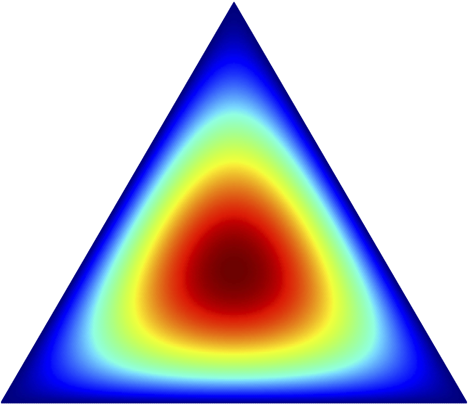
(a) The prior, $\text{Dir}(\pi|\alpha)$.

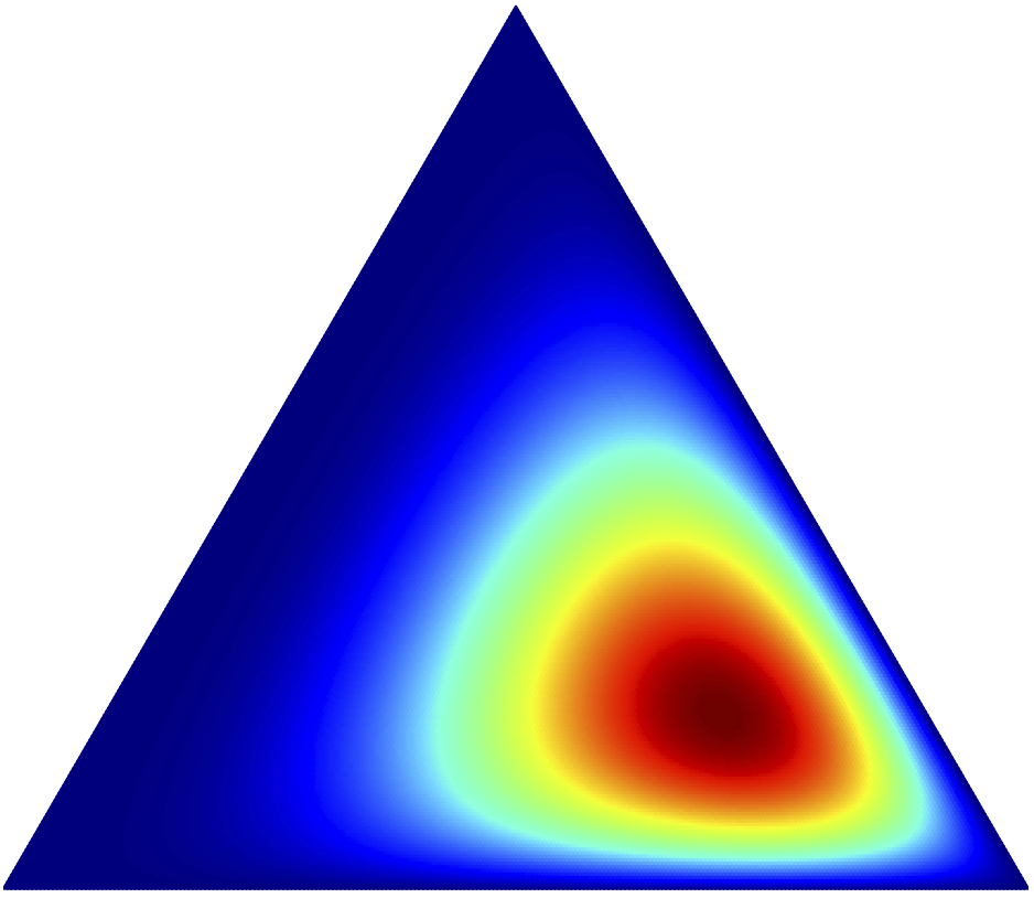
(b) The posterior proportional to $\text{Dir}(\pi|\alpha)\cdot\text{Mult}(m|\pi)$.

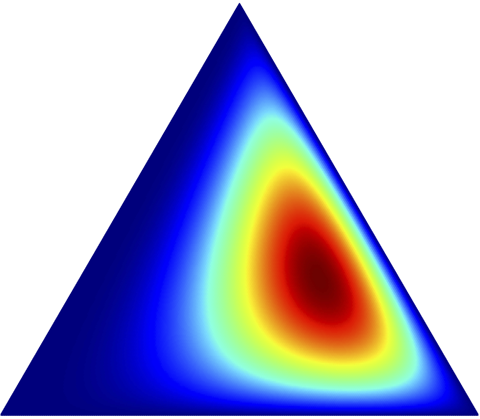
(c) The posterior proportional to $\text{Dir}(\pi|\alpha)\cdot\text{TruncMult}_{\{1\}}(m|\pi)$.

Figure 1: Projected visualizations of the prior distribution $\text{Dir}(\pi|\alpha)$ for $n=3$ and $\alpha=(2,2,2)$ and the associated posterior distributions when paired with $\text{Mult}(m|\pi)$ and $\text{TruncMult}_{\{1\}}(m|\pi)$ where $m=(0,2,0)$. In low dimensions, the posteriors can be computed via direct numerical integration over a discretized mesh.

3 An Auxiliary Variable Sampler

Data augmentation methods are auxiliary variable methods that often provide excellent sampling algorithms because they are easy to implement and the component steps are simply conjugate Gibbs sampling steps, resulting in fast mixing. For an overview, see the survey [6].

We can derive an auxiliary variable sampler for our problem by augmenting the distribution with geometric random variables $k=(k_{1},k_{2})=(\{k_{1j}\},\{k_{2j}\})$. That is, we define for $k_{ij}=\{0,1,2,\ldots\}$ a new distribution $q$ such that

$$q(\pi,m,k|\alpha) \propto\left(\prod_{i}\pi_{i}^{\alpha-1}\right)\left(\prod_{i\neq 1}\pi_{i}^{m_{1i}}\right)\left(\prod_{i\neq 2}\pi_{i}^{m_{2i}}\right)\left(\prod_{j=1}^{m_{1\cdot}}\pi_{1}^{k_{1j}}\right)\left(\prod_{j=1}^{m_{2\cdot}}\pi_{2}^{k_{2j}}\right)$$ (11)

where $\{m_{1i}\}$ and $\{m_{2i}\}$ are sample counts corresponding to each likelihood, respectively, and $m_{i\cdot}:=\sum_{j}m_{ij}$. Note that if we sum over all the auxiliary variables $k$, we have

$$\sum_{k}q(\pi,m,k|\alpha) \propto\left(\prod_{i}\pi_{i}^{\alpha-1}\right)\left(\prod_{i\neq 1}\pi_{i}^{m_{1i}}\right)\left(\prod_{i\neq 2}\pi_{i}^{m_{2i}}\right)\left(\prod_{j}\sum_{k_{1j}}\pi_{1}^{k_{1j}}\right)\left(\prod_{j}\sum_{k_{2j}}\pi_{2}^{k_{2j}}\right)$$ (12)

$$=\prod_{i}\pi_{i}^{\alpha-1}\left(\prod_{i\neq 1}\left(\frac{\pi_{i}}{1-\pi_{1}}\right)^{m_{1i}}\right)\left(\prod_{i\neq 2}\left(\frac{\pi_{i}}{1-\pi_{2}}\right)^{m_{2i}}\right)$$ (13)

$$\propto p(\pi,m|\alpha)$$ (14)

and so if we can construct samples of $\pi,k|m,\alpha$ from the distribution $q$ then we can form samples of $\pi|m,\alpha$ according to $p$ by simply ignoring the values sampled for $k$.

We construct samples of $\pi,k|m,\alpha$ by iterating Gibbs steps between $k|\pi,m,\alpha$ and $\pi|k,m,\alpha$. We see from (11) that each $k_{ij}$ in $k|\pi,m,\alpha=k|\pi,m$ is independent and distributed according to

$$q(k_{ij}|\pi,m) =(1-\pi_{i})\pi_{i}^{k_{ij}}.$$ (15)

Therefore, each $k_{ij}$ follows a geometric distribution with success parameter $(1-\pi_{i})$.

The distribution of $\pi|k,m,\alpha$ in $q$ is also simple:

$$q(\pi|m,k,\alpha) \propto\left(\prod_{i}\pi_{i}^{\alpha_{i}-1}\right)\left(\prod_{i\neq 1}\left(\frac{\pi_{i}}{1-\pi_{1}}\right)^{m_{1i}}\right)\left(\prod_{i\neq 2}\left(\frac{\pi_{i}}{1-\pi_{2}}\right)^{m_{2i}}\right)$$ (16)

$$\qquad\cdot\left(\prod_{j=1}^{m_{1\cdot}}(1-\pi_{1})\pi_{1}^{k_{1j}}\right)\left(\prod_{j=1}^{m_{2\cdot}}(1-\pi_{2})\pi_{2}^{k_{2j}}\right)$$ (17)

$$\propto\text{Dir}(\pi|\alpha+\tilde{m})$$ (18)

where $\tilde{m}$ is a set of augmented counts including the values of $k$. In other words, the Dirichlet prior is conjugate to the augmented model. Therefore we can cycle through Gibbs steps in the augmented distribution and hence easily produce samples from the desired posterior. For a graphical model of the augmentation, see Figure 2.

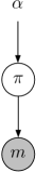
(a) Un-augmented distribution.

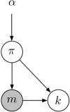
(b) Augmented distribution.

Figure 2: Graphical models for the un-augmented and augmented probability models.

4 Numerical Experiments

In this section we perform several numerical experiments to demonstrate the advantages provided by the auxiliary variable sampler. We compare to a generic Metropolis-Hastings sampling algorithm. For all experiments, when a statistic is computed in terms of a sampler chain’s samples up to sample index $t$, we discard the first $\lfloor\frac{t}{2}\rfloor$ samples and use the remaining samples to compute the statistic.

Metropolis-Hastings Sampler

We construct an MH sampling algorithm by using the proposal distribution which proposes a new position $\pi^{\prime}$ given the current position $\pi$ via the proposal distribution

$$p(\pi^{\prime}|\pi;\beta) =\text{Dir}(\pi^{\prime}|\beta\cdot\pi)$$ (19)

where $\beta>0$ is a tuning parameter. This proposal distribution has several valuable properties:

1. the mean and mode of the proposals are both $\pi$;

2. the parameter $\beta$ directly controls the concentration of the proposals, so that larger $\beta$ correspond to more local proposal samples;

3. the proposals are naturally confined to the support of the target distribution, while alternatives such as local Gaussian proposals would not satisfy the MH requirement that the normalization constant of the proposal kernel be constant for all starting points.

In our comparison experiments, we tune $\beta$ so that the acceptance probability is approximately $0.24$.

Sample Chain Autocorrelation

In Figure 3 we compare the sample autocorrelation of the auxiliary variable sampler and the alternative MH sampler for several lags with $n=10$. The reduced autocorrelation that is typical in the auxiliary variable sampler chain is indicative of faster mixing.

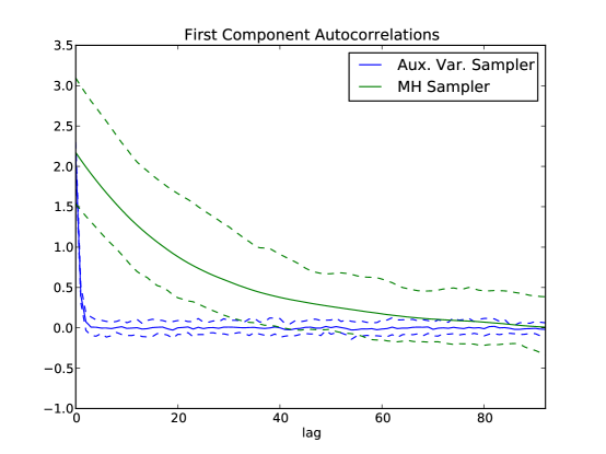
(a) Autocorrelations in the first (truncated) component.

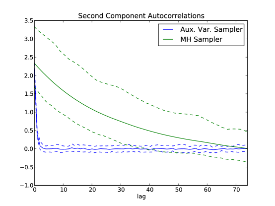
(b) Autocorrelations in the second component.

Figure 3: Autocorrelations for the auxiliary variable sampler and MH sampler chains with $\alpha_{i}=2$, $n=10$, $\beta=160$. The solid lines show the mean autocorrelation over 50 randomly-initialized runs for each sampler, and the dashed lines show the 10th and 90th percentile autocorrelation chains over those runs. These plots can be reproduced with the function autocorrelation in figures.py.

The $\widehat{R}$ Multivariate Potential Scale Reduction Factor

The $\widehat{R}$ statistic, also called the Multivariate Potential Scale Reduction Factor (MPSRF), was introduced in [1] and is a natural generalization of the scalar Scale Reduction Factor, introduced in [2] and discussed in [3, p. 296]. As a function of multiple independent sampler chains, the statistic compares the between-chain sample covariance matrix to the within-chain sample covariance matrix to measure mixing; good mixing is indicated by empirical convergence to the statistic’s asymptotic value of unity.

Specifically, loosely following the notation of [1], with $\psi_{jt}^{(i)}$ for denoting the $i$th element of the parameter vector in chain $j$ at time $t$ (with $i=1,\ldots,n$, $j=1,\ldots,M$, and $t=1,\ldots,T$), to compute the $n$-dimensional MPSRF we form

$$\widehat{V} =\frac{T-1}{T}W+\left(1+\frac{1}{M}\right)B/T$$ (20)

where

$$W =\frac{1}{M(T-1)}\sum_{j=1}^{M}\sum_{t=1}^{T}(\psi_{jt}-\bar{\psi}_{j\cdot})(\psi_{jt}-\bar{\psi}_{j\cdot})^{\mathsf{T}}$$ (21)

$$B/T =\frac{1}{M-1}\sum_{j=1}^{M}(\bar{\psi}_{j\cdot}-\bar{\psi}_{\cdot\cdot})(\bar{\psi}_{j\cdot}-\bar{\psi}_{\cdot c\cdot})^{\mathsf{T}}.$$ (22)

The MPSRF itself is then defined when $W$ is full-rank as [1, Eq. 4.1 and Lemma 1]

$$\widehat{R} :=\sup_{v\in\mathbb{R}^{n}}\frac{v^{\mathsf{T}}\widehat{V}v}{v^{\mathsf{T}}Wv}$$ (23)

$$=\lambda_{\text{max}}\left(W^{-1}\widehat{V}\right)$$ (24)

$$=\lambda_{\text{max}}\left(W^{-\frac{1}{2}}\widehat{V}W^{\frac{1}{2}}\right)$$ (25)

where $\lambda_{\text{max}}(A)$ denotes the eigenvalue of largest modulus of the matrix $A$ and the last line follows because conjugating by $W^{\frac{1}{2}}$ is a similarity transformation. Equivalently (and usefully for computation), we must find the largest solution $\lambda$ to $\det(\lambda W-\widehat{V})=0$.

However, as noted in [1, p. 446], the measure is incalculable when $W$ is singular, and because our samples are constrained to lie in the simplex in $n$ dimensions, the matrices involved will have rank $n-1$. Therefore when computing the $\widehat{R}$ statistic, we simply perform the natural Euclidean orthogonal projection to the $(n-1)$-dimensional affine subspace on which our samples lie; specifically, we define the statistic in terms of $Q^{\mathsf{T}}\widehat{V}Q$ and $Q^{\mathsf{T}}WQ$, where $Q$ is an $n\times(n-1)$ matrix such that $Q^{\mathsf{T}}Q=I_{(n-1)}$ and

$$QR =\begin{pmatrix}-(n-1)&1&\cdots&1&1\\ 1&-(n-1)&\cdots&1&1\\ &&\vdots&&\\ 1&1&\cdots&1&-(n-1)\\ 1&1&\cdots&1&1\\ \end{pmatrix}$$ (26)

for upper-triangular $R$ of size $(n-1)\times(n-1)$.

Figure 4 shows the MPSRF of both samplers computed over 50 sample chains for $n=10$ dimensions, and Figure 5 shows the even greater performance advantage of the auxiliary variable sampler in higher dimensions.

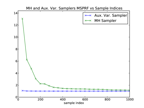
(a) The horizontal axis is the sample index.

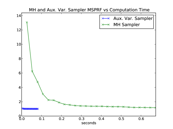
(b) The horizontal axis is elapsed time.

Figure 4: The $\widehat{R}$ Multivariate Potential Scale Reduction Factor [1] for the auxiliary variable sampler and MH sampler with $\alpha_{i}=2$, $n=10$, and $\beta=160$, with horizontal axes scaled by sample index and elapsed time. For each sampler, 5000 samples were drawn for each of 50 randomly-initialized runs, and the MPSRF was computed at 25 equally-spaced intervals. These plots can be reproduced with the function Rhatp in figures.py.

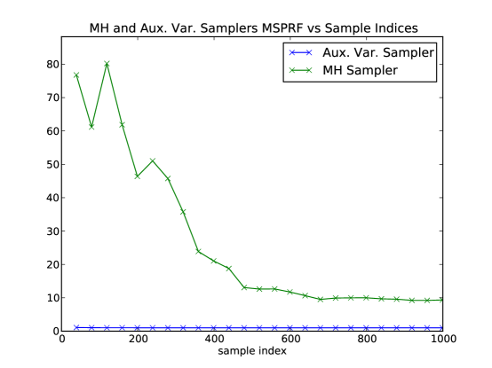
(a) The horizontal axis is the sample index.

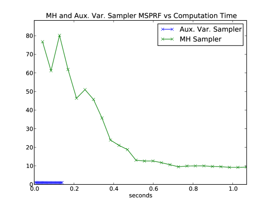
(b) The horizontal axis is elapsed time.

Figure 5: The $\widehat{R}$ Multivariate Potential Scale Reduction Factor [1] for the auxiliary variable sampler and MH sampler with $\alpha_{i}=2$, $n=20$, and $\beta=160$, with horizontal axes scaled by sample index and elapsed time. For each sampler, 5000 samples were drawn for each of 50 randomly-initialized runs, and the MPSRF was computed at 25 equally-spaced intervals. These plots can be reproduced with the function Rhatp in figures.py.

Statistic Convergence

Finally, we show the convergence of the component-wise mean and variance statistics for the two samplers. We estimated the true statistics by forming estimates using samples from 50 independent chains each with 5000 samples, effectively using 250000 samples to form the estimates. Next, we plotted the $\ell_{2}$ distance between these “true” statistic vectors and those estimated at several sample indices along the 50 runs for each of the sampling algorithms. See the plots in Figure 6.

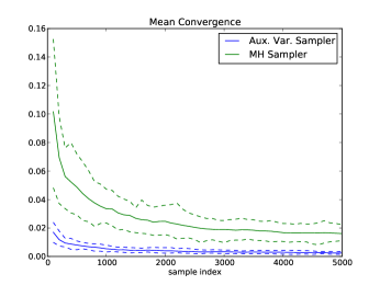
(a) $\ell_{2}$ error of component-wise mean estimate vs sample index.

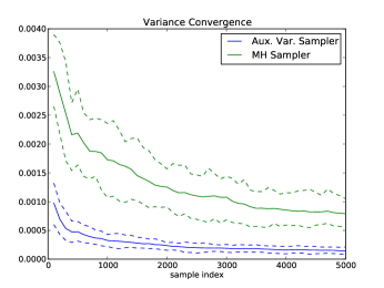
(b) $\ell_{2}$ error of component-wise variance estimate vs sample index.

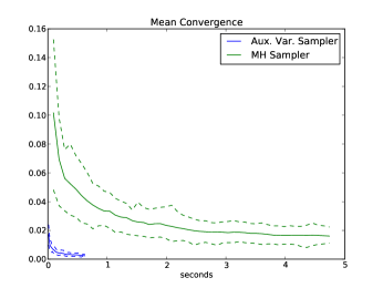
(c) $\ell_{2}$ error of component-wise mean estimate vs elapsed time.

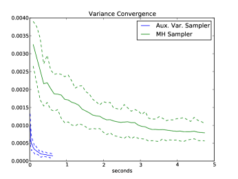
(d) $\ell_{2}$ error of component-wise variance estimate vs elapsed time.

Figure 6: Component-wise statistic convergence for the auxiliary variable sampler and MH sampler with $\alpha_{i}=2$, $n=10$, and $\beta=160$, with horizontal axes scaled by sample index and elapsed time. For each sampler, 5000 samples were drawn for each of 50 randomly-initialized runs. The $\ell_{2}$ distances from estimated “true” parameters are plotted, with the solid lines corresponding to the mean error and the dashed lines corresponding to 10th and 90th percentile errors. These plots can be reproduced with the function statistic_convergence in figures.py.

References

- [1] S.P. Brooks and A. Gelman “General Methods for Monitoring Convergence of Iterative Simulations” In Journal of Computational and Graphical Statistics JSTOR, 1998, pp. 434–455
- [2] A. Gelman and D.B. Rubin “Inference from iterative simulation using multiple sequences” In Statistical science 7.4 Institute of Mathematical Statistics, 1992, pp. 457–472
- [3] A. Gelman, J.B. Carlin, H.S. Stern and D.B. Rubin “Bayesian Data Analysis” CRC press, 2004
- [4] Matthew J. Johnson and Alan S. Willsky “Bayesian Nonparametric Hidden Semi-Markov Models” In Preprint arXiv:1203.1365v1 [stat.ME]
- [5] P. Orbanz “Construction of nonparametric Bayesian models from parametric Bayes equations” In Advances in Neural Information Processing Systems, 2009
- [6] D.A. Van Dyk and X.L. Meng “The Art of Data Augmentation” In Journal of Computational and Graphical Statistics 10.1 ASA, 2001, pp. 1–50