Convergence of a fully discrete finite difference scheme for the Korteweg–de Vries equation

Abstract.

We prove convergence of a fully discrete finite difference scheme for the Korteweg–de Vries equation. Both the decaying case on the full line and the periodic case are considered. If the initial data $u|_{t=0}=u_{0}$ is of high regularity, $u_{0}\in H^{3}(\mathbb{R})$, the scheme is shown to converge to a classical solution, and if the regularity of the initial data is smaller, $u_{0}\in L^{2}(\mathbb{R})$, then the scheme converges strongly in $L^{2}(0,T;L^{2}_{\mathrm{loc}}(\mathbb{R}))$ to a weak solution.

1. Introduction

The Korteweg–de Vries (KdV among friends and foes) equation, which reads

(1.1) $$u_{t}+uu_{x}+u_{xxx}=0,$$

has been studied extensively since its first analysis in 1895 by Korteweg and de Vries. Apart from applications as a model for shallow water waves, the KdV equation has maintained a pivotal role in several branches of mathematics. We here focus on the derivation of convergent numerical methods for the initial value problem where the equation (1.1) is augmented by initial data $u|_{t=0}=u_{0}$. The problem of analyzing convergent numerical schemes is of course intimately connected with the mathematical properties of the Cauchy problem for the KdV equation, which has undergone a tremendous development the last two decades, see, e.g., [17, 14] and the references therein. We will not be able to discuss this literature here, but only refer to the parts that are pertinent to the current paper.

In this paper we analyze the implicit finite difference scheme

(1.2) $$u^{n+1}_{j}=\overline{u}^{n}_{j}-{\Delta t}\,\overline{u}^{n}_{j}Du^{n}_{j}-{\Delta t}\,D_{+}^{2}D_{-}u^{n+1}_{j},\quad n\in\mathbb{N}_{0},\,j\in\mathbb{Z},$$

where $u^{n}_{j}\approx u(j{\Delta x},n{\Delta t})$, and ${\Delta x},{\Delta t}$ are small discretization parameters. Furthermore, $D$ and $D_{\pm}$ denote symmetric and forward/backward (spatial) finite differences, respectively, and $\overline{u}$ denotes a spatial average. Two results are proven, both for the full line and the periodic case: (1) In the case of initial data $u_{0}\in H^{3}(\mathbb{R})$, we show (see Theorem 3.3 and Remark 3.4) that the approximation (1.2) converges uniformly as ${\Delta x}\to 0$ with ${\Delta t}=\mathcal{O}\left({\Delta x}^{2}\right)$ in $C(\mathbb{R}\times[0,\bar{T}])$ for any positive $\bar{T}$ to the unique solution of the KdV equation. (2) When the initial data $u_{0}\in L^{2}(\mathbb{R})$, we prove that (see Theorem 4.3) that the approximation converges strongly as ${\Delta x}\to 0$ with ${\Delta t}=\mathcal{O}\left({\Delta x}^{2}\right)$ in $L^{2}(0,T;L^{2}_{\mathrm{loc}}(\mathbb{R}))$ to a weak solution of the KdV equation.

An interesting fact, and rarely referred to in the current literature, is that the first mathematical proof of existence and uniqueness of solutions of the KdV equation, was accomplished by Sjöberg [16] in 1970, using a finite difference approximation very much in the spirit considered here. His proof is valid for initial data that are periodic and with square integrable third derivative, that is, $u_{0}(x+1)=u_{0}(x)$ for $x\in[0,1]$ and $u_{0}^{\prime\prime\prime}\in L^{2}([0,1])$. Sjöberg’s uniqueness proof still is the standard one, using the Gronwall inequality. His approach is based on a semi-discrete approximation where one discretizes the spatial variable, thereby reducing the equation to a system of ordinary differential equations. However, we stress that for numerical computations also this set of ordinary differential equations will have to be discretized in order to be solved. Thus in order to have a completely satisfactory numerical method, one seeks a fully discrete scheme that reduces the actual computation to a solution of a finite set of algebraic equations. This is accomplished in the present paper, both in the periodic case and on the full line.

There has been a number of papers involving the numerical computation of solutions of the Cauchy problem, starting with the landmark paper by Zabusky and Kruskal [20], where they discovered the permanence of solitons (the term “solitons” being coined in the same paper) for the KdV equation using numerical techniques. However, we will here focus on papers that discuss numerical methods per se.

A popular numerical approach has been the application of various spectral methods. Little is known rigorously about the convergence of these methods. For a survey and a comparison, see [15]. See also [12]. Multisymplectic schemes have been studied in [3] (see also references therein). There exist convergence proofs for finite element methods for the KdV equation, see [19, 2, 4, 5]. However, the resulting schemes tend to be quite different from finite difference schemes derived ab initio.

The numerical computation of solutions of the KdV equation is rather capricious. Two competing effects are involved, namely the nonlinear convective term $uu_{x}$, which in the context of the Burgers equation $u_{t}+uu_{x}=0$ yields infinite gradients in finite time even for smooth data, and the linear dispersive term $u_{xxx}$, which in the Airy equation $u_{t}+u_{xxx}=0$ produces hard-to-compute dispersive waves, and these two effects combined makes it difficult to obtain accurate and fast numerical methods. Indeed, any initial data for the Burgers equation that is decreasing in a small neighborhood, will develop infinite gradients in finite time, while the Airy equation preserves all Sobolov norms while creating many oscillatory waves. Most finite difference schemes will consist of a sum of two terms, one discretizing the convective term and one discretizing the dispersive term. These two effects will have to balance each other, as it is known that the KdV equation itself keeps the Sobolov norm $H^{s}$ bounded; from [6] we know that if $u_{0}\in H^{s}(\mathbb{R})$, with $s\geq 3$, then the solution satisfies $\left\|u(t)\right\|_{H^{s}(\mathbb{R})}\leq C_{T,u_{0}}$ for $t\in[0,T]$. This dichotomy between these two effects is brought to the forefront in the method of operator splitting. Here the two equations, the Burgers equations and the Airy equation, are solved sequentially for a small time step. This procedure is iterated, and as the time step converges to zero, the approximation converges to the actual solution. In the KdV context operator splitting was introduced by Tappert [18], a Lax–Wendroff theorem was proved in [7], and convergence of the operator splitting technique proved in [8, 11, 9, 10]. Our approach here is a finite difference method which can also be viewed as an operator splitting method.

Recently, a semi-discrete scheme for the generalized KdV equation was shown to converge in $L^{2}_{\mathrm{loc}}$ for initial data in $L^{2}$ [1]. However, the scheme analyzed here, which in contrast to the scheme in [1], does not involve an explicit fourth order stabilizing term, and we show convergence for non-smooth initial data.

The rest of this paper is organized as follows: In Section 2 we present the necessary notation and define the numerical scheme. In Section 3 we show the convergence of the scheme for initial data in $H^{3}(\mathbb{R})$, while in Section 4 we show the convergence to a weak solution if the initial data is in $L^{2}(\mathbb{R})$. In Section 5 we exhibit some numerical experiments showing the convergence.

2. The scheme

We start by introducing the necessary notation. Derivatives will be approximated by finite differences, and the basic quantities are as follows. For any function $p\colon\mathbb{R}\to\mathbb{R}$ we set

$$D_{\pm}p(x)=\pm\frac{1}{{\Delta x}}\big{(}p(x\pm{\Delta x})-p(x)\big{)},\ \text{and}\ D=\frac{1}{2}\left(D_{+}+D_{-}\right)$$

for some (small) positive number ${\Delta x}$. If we introduce the average

$$\overline{p}(x)=\frac{1}{2}\left(p(x+{\Delta x})+p(x-{\Delta x})\right),$$

we find the Leibniz rule as

$$D(pq) =\overline{p}Dq+\overline{q}Dp,$$

$$D_{\pm}(pq) =S^{\pm}pD_{\pm}q+qD_{\pm}p=S^{\pm}qD_{\pm}p+pD_{\pm}q.$$

Here we have defined the shift operator

$$S^{\pm}p(x)=p(x\pm{\Delta x}).$$

We discretize the real axis using ${\Delta x}$ and set $x_{j}=j{\Delta x}$ for $j\in\mathbb{Z}$. For a given function $p$ we define $p_{j}=p(x_{j})$. We will consider functions in $\ell^{2}$ with the usual inner product and norm

$$(p,q)={\Delta x}\sum_{j\in\mathbb{Z}}p_{j}q_{j},\quad\left\|p\right\|=(p,p)^{1/2},\qquad p,q\in\ell^{2}.$$

In the periodic case with period $J$ the sum over $\mathbb{Z}$ is replaced by a finite sum $j=0,\dots,J-1$. Observe that

$$\left\|p\right\|_{\infty}=\max_{j\in\mathbb{Z}}\left|p_{j}\right|\leq\frac{1}{{\Delta x}^{1/2}}\left\|p\right\|.$$

The various difference operators enjoy the following properties:

$$(p,D_{\pm}q)=-(D_{\mp}p,q),\quad(p,Dq)=-(Dp,q),\qquad p,q\in\ell^{2}.$$

Further useful properties include

(2.1) $$(u,D_{+}^{2}D_{-}u) =\frac{1}{2}(u,D_{-}D_{+}^{2}u)-\frac{1}{2}(u,D_{+}D_{-}^{2}u)$$

$$=\frac{1}{2}\big{(}u,(D_{-}D_{+}^{2}-D_{+}D_{-}^{2})u\big{)}$$

$$=\frac{1}{2}\big{(}u,D_{-}D_{+}(D_{-}-D_{+})u\big{)}$$

$$=\frac{{\Delta x}}{2}\left\|D_{+}D_{-}u\right\|^{2}$$

since $(u,D_{+}D_{-}^{2}u)=-(u,D_{-}D_{+}^{2}u)$ (because $(u,v)=(v,u)$) in the first line, and

$$D_{-}-D_{+}=-{\Delta x}\,D_{+}D_{-}=-{\Delta x}\,D_{-}D_{+}.$$

We also need to discretize in the time direction. Introduce (a small) time step ${\Delta t}>0$, and use the notation

$$D^{t}_{+}p(t)=\frac{1}{{\Delta t}}\big{(}p(t+{\Delta t})-p(t)\big{)},$$

for any function $p\colon[0,T]\to\mathbb{R}$. Write $t_{n}=n{\Delta t}$ for $n\in\mathbb{N}_{0}=\mathbb{N}\cup\{0\}$. A fully discrete grid function is a function $u_{\Delta x}\colon{\Delta t}\,\mathbb{N}_{0}\to\mathbb{R}^{\mathbb{Z}}$, and we write $u_{\Delta x}(x_{j},t_{n})=u^{n}_{j}$. (A CFL condition will enforce a relationship between ${\Delta x}$ and ${\Delta t}$, and hence we only use ${\Delta x}$ in the notation.)

We propose the following implicit scheme to generate approximate solutions to the KdV equation (1.1)

(2.2) $$u^{n+1}_{j}=\overline{u}^{n}_{j}-{\Delta t}\,\overline{u}^{n}_{j}Du^{n}_{j}-{\Delta t}\,D_{+}^{2}D_{-}u^{n+1}_{j},\quad n\in\mathbb{N}_{0},\,j\in\mathbb{Z}.$$

For the initial data we have

$$u^{0}_{j}=u_{0}(x_{j}),\quad j\in\mathbb{Z}.$$

Remark 2.1.

This scheme can be reformulated as an operator splitting scheme as follows. Set

$$u^{n+1/2}_{j}=\frac{1}{2}\left(u^{n}_{j+1}+u^{n}_{j-1}\right)-\frac{{\Delta t}}{2{\Delta x}}\left(\frac{1}{2}\left(u^{n}_{j+1}\right)^{2}-\frac{1}{2}\left(u^{n}_{j-1}\right)^{2}\right),$$

i.e., $u^{n+1/2}$ is solution operator of the Lax–Friedrichs scheme for Burgers’ equation, applied to $u^{n}$. Then

$$\frac{u^{n+1}-u^{n+1/2}}{{\Delta t}}=-D_{+}^{2}D_{-}u^{n+1},$$

i.e., $u^{n+1}$ is the approximate solution operator of a first-order implicit scheme for Airy’s equation $u_{t}+u_{xxx}=0$. If we write these two approximate solution operators as $S^{B}_{{\Delta t}}$, and $S^{A}_{\Delta t}$, respectively, the update formula (2.2) reads

$$u^{n+1}=\left(S_{\Delta t}^{A}\circ S_{\Delta t}^{B}\right)u^{n}.$$

The convergence of this type of operator splitting using exact solution operators have been shown in [8, 11], with severe restrictions on the initial data. The results in this paper can be viewed as a convergence result for operator splitting using approximate operators with less restrictions on the initial data, but with specified ratios between the temporal and spatial discretizations (CFL-like conditions).

3. Convergence for smooth initial data

To show that the implicit scheme can be solved with respect to $u^{n+1}_{j}$, we proceed as follows: Write the scheme as

$$(1+{\Delta t}D_{+}^{2}D_{-})u^{n+1}_{j}=\overline{u}^{n}_{j}-{\Delta t}\,\overline{u}^{n}_{j}Du^{n}_{j}$$

and hence

$$((1+{\Delta t}D_{+}^{2}D_{-})u^{n+1},u^{n+1}) =\left\|u^{n+1}\right\|^{2}+{\Delta t}(D_{+}^{2}D_{-}u^{n+1},u^{n+1})$$

$$=\left\|u^{n+1}\right\|^{2}+\frac{1}{2}{\Delta t}{\Delta x}\left\|D_{+}D_{-}u^{n+1}\right\|^{2}$$

$$\geq\left\|u^{n+1}\right\|^{2},$$

thus

$$\left\|u^{n+1}\right\|\leq\left\|(1+{\Delta t}D_{+}^{2}D_{-})u^{n+1}\right\|=\left\|\overline{u}^{n}-{\Delta t}\,\overline{u}^{n}Du^{n}\right\|.$$

The fundamental stability lemma reads as follows.

Lemma 3.1.

Let $u^{n}_{j}$ be a solution of the difference scheme (2.2). Then the following estimate holds

(3.1) $$\left\|u^{n+1}\right\|^{2}+{\Delta t}{\Delta x}^{1/2}\Big{(}{\Delta x}\lambda\left\|D_{+}^{2}D_{-}u^{n+1}\right\|^{2}+{\Delta x}^{1/2}\left\|D_{+}D_{-}u^{n+1}\right\|^{2}+\frac{\delta}{\lambda}\left\|Du^{n}\right\|^{2}\Big{)}\\ \leq\left\|u^{n}\right\|^{2},$$

provided the CFL condition

(3.2) $$\lambda\left\|u^{0}\right\|\left(\frac{1}{3}+\frac{1}{2}\lambda\left\|u^{0}\right\|\right)<\frac{1-\delta}{2},\quad\delta\in(0,1),$$

holds where $\lambda={\Delta t}/{\Delta x}^{3/2}$.

Proof.

For the moment we drop the indices $j$ and $n$ from our notation, and use the notation $u$ for $u_{j}^{n}$ where $j$ and $n$ are fixed. We first study the “Burgers” term ${\Delta t}\,\overline{u}Du$. Let $u$ be a grid function and set

(3.3) $$w=\overline{u}-{\Delta t}\,\overline{u}Du.$$

If the timestep ${\Delta t}$ satisfies (3.2) then we have the following “cell entropy” inequality

(3.4) $$\frac{1}{2}w^{2}\leq\frac{1}{2}\overline{u^{2}}-\frac{{\Delta t}}{3}Du^{3}-\delta\frac{{\Delta x}^{2}}{2}\left(Du\right)^{2},\quad\delta\in(0,1).$$

To prove this we multiply (3.3) by $\overline{u}$ to find

$$\frac{1}{2}w^{2} =\frac{1}{2}\overline{u}^{2}-{\Delta t}\frac{1}{2}\overline{u}Du^{2}+\frac{1}{2}\left(w-\overline{u}\right)^{2}$$

$$=\frac{1}{2}\overline{u^{2}}-{\Delta t}\frac{1}{2}\overline{u}Du^{2}+\frac{1}{2}{\Delta t}^{2}\overline{u}^{2}\left(Du\right)^{2}+\frac{1}{2}\left(\overline{u}^{2}-\overline{u^{2}}\right).$$

Now we have that

$$\frac{1}{4}(a+b)\left(a^{2}-b^{2}\right)=\frac{1}{3}\left(a^{3}-b^{3}\right)-\frac{1}{12}(a-b)^{3},$$

and

$$\frac{1}{4}(a+b)^{2}-\frac{1}{2}\left(a^{2}+b^{2}\right)=-\frac{1}{4}(a-b)^{2}.$$

For a grid function, this implies

$$\overline{u}Du^{2} =\frac{2}{3}Du^{3}-\frac{2{\Delta x}^{2}}{3}\left(Du\right)^{3},$$

$$\overline{u}^{2}-\overline{u^{2}} =-{\Delta x}^{2}\left(Du\right)^{2}.$$

Therefore

$$\frac{1}{2}w^{2} =\frac{1}{2}\overline{u^{2}}-\frac{{\Delta t}}{3}Du^{3}+\frac{1}{2}{\Delta t}^{2}\overline{u}^{2}\left(Du\right)^{2}+\frac{{\Delta t}{\Delta x}^{2}}{3}\left(Du\right)^{3}-\frac{{\Delta x}^{2}}{2}\left(Du\right)^{2}$$

$$=\frac{1}{2}\overline{u^{2}}-\frac{{\Delta t}}{3}Du^{3}-\delta\frac{{\Delta x}^{2}}{2}\left(Du\right)^{2}$$

$$\qquad+{\Delta x}^{2}\left(Du\right)^{2}\left(\frac{\lambda}{3}{\Delta x}^{3/2}Du+\frac{1}{2}{\Delta x}\lambda^{2}\overline{u}^{2}-\frac{1-\delta}{2}\right)$$

$$\leq\frac{1}{2}\overline{u^{2}}-\frac{{\Delta t}}{3}Du^{3}-\delta\frac{{\Delta x}^{2}}{2}\left(Du\right)^{2}$$

$$\qquad+{\Delta x}^{2}\left(Du\right)^{2}\left(\frac{\lambda}{3}{\Delta x}^{1/2}\left\|u\right\|_{\infty}+\frac{1}{2}{\Delta x}\lambda^{2}\overline{u}^{2}-\frac{1-\delta}{2}\right)$$

$$\leq\frac{1}{2}\overline{u^{2}}-\frac{{\Delta t}}{3}Du^{3}-\delta\frac{{\Delta x}^{2}}{2}\left(Du\right)^{2}$$

$$\qquad+{\Delta x}^{2}\left(Du\right)^{2}\underbrace{\left(\frac{\lambda}{3}\left\|u\right\|+\frac{1}{2}\lambda^{2}\left\|u\right\|^{2}-\frac{1-\delta}{2}\right)}_{A}$$

$$\leq\frac{1}{2}\overline{u^{2}}-\frac{{\Delta t}}{3}Du^{3}-\delta\frac{{\Delta x}^{2}}{2}\left(Du\right)^{2},\quad\delta\in(0,1),$$

where we have employed that $A<0$ since $\lambda$ satisfies the CFL condition (3.2). Estimate (3.4) follows.

Summing (3.4) over $j$ we get

(3.5) $$\left\|w\right\|^{2}+\delta{\Delta x}^{2}\left\|Du\right\|^{2}\leq\left\|u\right\|^{2}.$$

Next we study the full difference scheme by adding the “Airy term” ${\Delta t}\,D_{+}^{2}D_{-}u^{n+1}_{j}$. Thus the full difference scheme (2.2) can be written

$$v=w-{\Delta t}\,D_{+}^{2}D_{-}v.$$

Writing this as $w=v+{\Delta t}\,D_{+}^{2}D_{-}v$, we square it and sum over $j$ to get

(3.6) $$\left\|w\right\|^{2} =\left\|v\right\|^{2}+2{\Delta t}(v,D_{+}^{2}D_{-}v)+{\Delta t}^{2}\left\|D_{+}^{2}D_{-}v\right\|^{2}$$

$$=\left\|v\right\|^{2}+{\Delta t}{\Delta x}\left\|D_{-}D_{+}v\right\|^{2}+{\Delta t}^{2}\left\|D_{+}^{2}D_{-}v\right\|^{2},$$

using the identity (2.1).

For the function $u^{n}$ this means that

(3.7) $$\left\|w\right\|^{2} =\left\|u^{n+1}\right\|^{2}$$

$$\qquad+{\Delta t}{\Delta x}^{1/2}\left({\Delta x}\lambda\left\|D_{+}^{2}D_{-}u^{n+1}\right\|^{2}+{\Delta x}^{1/2}\left\|D_{+}D_{-}u^{n+1}\right\|^{2}\right)$$

$$\leq\left\|u^{n}\right\|^{2}-\delta{\Delta x}^{2}\left\|Du\right\|^{2},$$

using (3.5). This implies

(3.8) $$\left\|u^{n+1}\right\|^{2}+{\Delta t}{\Delta x}^{1/2}\big{(}{\Delta x}\lambda\left\|D_{+}^{2}D_{-}u^{n+1}\right\|^{2}\\ +{\Delta x}^{1/2}\left\|D_{+}D_{-}u^{n+1}\right\|^{2}+\frac{\delta}{\lambda}\left\|Du^{n}\right\|^{2}\big{)}\leq\left\|u^{n}\right\|^{2}.$$

∎

Next, we consider what corresponds to the finite difference scheme satisfied by the time derivative of the original scheme.

Lemma 3.2.

Let $u^{n}_{j}$ be a solution of the difference scheme (2.2). Then the following estimate holds

(3.9) $$\left\|D^{t}_{+}u^{n}\right\|^{2} +{\Delta t}^{2}\left\|D_{+}^{2}D_{-}D^{t}_{+}u^{n}\right\|^{2}$$

$$+{\Delta t}{\Delta x}\left\|D_{+}D_{-}D^{t}_{+}u^{n}\right\|^{2}+\tilde{\delta}{\Delta x}^{2}\left\|DD^{t}_{+}u^{n-1}\right\|^{2}$$

$$\qquad\qquad\qquad\qquad\qquad\leq\left\|D^{t}_{+}u^{n-1}\right\|^{2}\left(1+3{\Delta t}\left\|Du^{n}\right\|_{\infty}\right),$$

provided ${\Delta t}$ is chosen such that

(3.10) $$6\left\|u_{0}\right\|^{2}\lambda^{2}+\left\|u_{0}\right\|\lambda<\frac{1-\tilde{\delta}}{2},\qquad\tilde{\delta}\in(0,1).$$

Proof.

Introduce

$$\alpha^{n}=D^{t}_{+}u^{n-1}=\frac{1}{{\Delta t}}(u^{n}-u^{n-1}),\quad n\in\mathbb{N}.$$

Using (2.2) we see that this grid function satisfies

$$\alpha^{n+1} =\overline{\alpha}^{n}-{\Delta t}\left(\overline{\alpha}^{n}Du^{n}+\overline{u}^{n-1}D\ \alpha^{n}\right)+{\Delta t}^{2}\overline{\alpha}^{n}D\alpha^{n}-{\Delta t}D_{+}^{2}D_{-}\alpha^{n+1}$$

(3.11) $$=\overline{\alpha}^{n}-{\Delta t}\,D(u^{n}\alpha^{n})+{\Delta t}^{2}\overline{\alpha}^{n}D\alpha^{n}-{\Delta t}D_{+}^{2}D_{-}\alpha^{n+1},\quad n\in\mathbb{N}.$$

Introduce

(3.12) $$\beta=\overline{\alpha}-{\Delta t}\,D(u\alpha)+\frac{{\Delta t}^{2}}{2}D\alpha^{2},$$

which means that (3.11) can be written as

(3.13) $$\alpha^{n+1}=\beta-{\Delta t}D_{+}^{2}D_{-}\alpha^{n+1}.$$

We proceed as before and square (3.12) to find

$$\frac{1}{2}\beta^{2} =\frac{1}{2}\overline{\alpha^{2}}+\frac{{\Delta t}^{2}}{2}\left(D(u\alpha)-\frac{{\Delta t}}{2}D\alpha^{2}\right)^{2}$$

$$\qquad-{\Delta t}\left(\overline{u}\,\overline{\alpha}D\alpha+\overline{\alpha}^{2}Du\right)+{\Delta t}^{2}\overline{\alpha}^{2}D\alpha-\frac{{\Delta x}^{2}}{2}\left(D\alpha\right)^{2}.$$

We have that

$$\frac{1}{2}\left(D(u\alpha)-\frac{{\Delta t}}{2}D\alpha^{2}\right)^{2} \leq\left(D(u\alpha)\right)^{2}+{\Delta t}^{2}\overline{\alpha}^{2}\left(D\alpha\right)^{2}$$

$$\leq 2\overline{u}^{2}\left(D\alpha\right)^{2}+2\overline{\alpha}^{2}\left(Du\right)^{2}+{\Delta t}^{2}\overline{\alpha}^{2}\left(D\alpha\right)^{2},$$

$$\overline{\alpha}^{2}D\alpha =\frac{1}{3}D\alpha^{3}-\frac{{\Delta x}^{2}}{3}\left(D\alpha\right)^{3},$$

$$\overline{u}\,\overline{\alpha}D\alpha+\overline{\alpha}^{2}Du =\frac{1}{2}D\left(u\alpha^{2}\right)+\frac{1}{2}\overline{\alpha}^{2}Du-\frac{{\Delta x}^{2}}{2}\left(D\alpha\right)^{2}Du.$$

Using this

(3.14) $$\frac{1}{2}\beta^{2} \leq\frac{1}{2}\overline{\alpha^{2}}-\frac{{\Delta t}}{2}D\left(u\alpha^{2}-\frac{2{\Delta t}}{3}\alpha^{3}\right)-\frac{{\Delta t}}{2}\overline{\alpha}^{2}Du+\frac{{\Delta t}{\Delta x}^{2}}{2}\left(D\alpha\right)^{2}Du$$

$$\quad+{\Delta t}^{2}\left(2\overline{u}^{2}\left(D\alpha\right)^{2}+2\overline{\alpha}^{2}\left(Du\right)^{2}+{\Delta t}^{2}\overline{\alpha}^{2}\left(D\alpha\right)^{2}-\frac{{\Delta x}^{2}}{3}\left(D\alpha\right)^{3}\right)$$

$$\quad-\frac{{\Delta x}^{2}}{2}\left(D\alpha\right)^{2}.$$

Now we must balance the positive terms with ${\Delta x}^{2}(D\alpha)^{2}$. To this end we estimate

$${\Delta x}^{2}(D\alpha)^{2} \leq\overline{\alpha^{2}},$$

$${\Delta t}^{2}\overline{\alpha}^{2}(Du)^{2} \leq\lambda{\Delta x}^{1/2}\,{\Delta t}\left\|u^{n}\right\|_{\infty}\overline{\alpha^{2}}\left|Du^{n}\right|,$$

$${\Delta t}^{2}\overline{\alpha}^{2} \leq 2\left\|u^{n}\right\|_{\infty}^{2}+2\left\|u^{n-1}\right\|_{\infty}^{2},$$

$${\Delta x}^{2}\left|D\alpha\right| \leq\frac{1}{\lambda{\Delta x}^{1/2}}\left(\left\|u^{n}\right\|_{\infty}+\left\|u^{n-1}\right\|_{\infty}\right).$$

Using these in (3.14) we find

$$\frac{1}{2}\beta^{2} \leq\frac{1}{2}\overline{\alpha^{2}}-\frac{{\Delta t}}{2}D\left(u\alpha^{2}-\frac{2{\Delta t}}{3}\alpha^{3}\right)+(\frac{{\Delta t}}{2}+\frac{{\Delta t}}{2})\overline{\alpha^{2}}\left|Du\right|+2{\Delta t}^{2}\,\overline{\alpha}^{2}(Du)^{2}$$

$$\quad+\lambda^{2}{\Delta x}^{3}\left(D\alpha\right)^{2}\left(2\overline{u}^{2}+2\left\|u^{n}\right\|_{\infty}^{2}+2\left\|u^{n-1}\right\|_{\infty}^{2}+\frac{1}{3\lambda{\Delta x}^{1/2}}\left(\left\|u^{n}\right\|_{\infty}+\left\|u^{n-1}\right\|_{\infty}\right)\right)$$

$$\quad-\frac{{\Delta x}^{2}}{2}\left(D\alpha\right)^{2}$$

$$\leq\frac{1}{2}\overline{\alpha^{2}}-\frac{{\Delta t}}{2}D\left(u\alpha^{2}-\frac{2{\Delta t}}{3}\alpha^{3}\right)+{\Delta t}\left(1+\lambda{\Delta x}^{1/2}\,\left\|u^{n}\right\|_{\infty}\right)\overline{\alpha^{2}}\left|Du^{n}\right|$$

$$\quad+\lambda^{2}{\Delta x}^{2}\left(D\alpha\right)^{2}\left(2{\Delta x}\left(2\left\|u^{n}\right\|_{\infty}^{2}+\left\|u^{n-1}\right\|_{\infty}^{2}\right)+\frac{{\Delta x}^{1/2}}{3\lambda}\left(\left\|u^{n}\right\|_{\infty}+\left\|u^{n-1}\right\|_{\infty}\right)\right)$$

$$\quad-\frac{{\Delta x}^{2}}{2}\left(D\alpha\right)^{2}$$

$$\leq\frac{1}{2}\overline{\alpha^{2}}-\frac{{\Delta t}}{2}D\left(u\alpha^{2}-\frac{2{\Delta t}}{3}\alpha^{3}\right)+{\Delta t}(1+\lambda\left\|u_{0}\right\|)\overline{\alpha^{2}}\left|Du^{n}\right|$$

$$\quad+\lambda^{2}{\Delta x}^{2}\left(D\alpha\right)^{2}\left(6\left\|u_{0}\right\|^{2}+\frac{2}{3\lambda}\left\|u_{0}\right\|-\frac{1-\tilde{\delta}}{2\lambda^{2}}\right)-\tilde{\delta}\frac{{\Delta x}^{2}}{2}\left(D\alpha\right)^{2}$$

$$\leq\frac{1}{2}\overline{\alpha^{2}}-\frac{{\Delta t}}{2}D\left(u\alpha^{2}-\frac{2{\Delta t}}{3}\alpha^{3}\right)+{\Delta t}\frac{3-\tilde{\delta}}{2}\,\overline{\alpha^{2}}\left|Du^{n}\right|$$

$$\quad+{\Delta x}^{2}\left(D\alpha\right)^{2}\left(6\left\|u_{0}\right\|^{2}\lambda^{2}+\left\|u_{0}\right\|\lambda-\frac{1-\tilde{\delta}}{2}\right)-\tilde{\delta}\frac{{\Delta x}^{2}}{2}\left(D\alpha\right)^{2},\quad\tilde{\delta}\in(0,1).$$

Here we have enforced the CFL condition (3.10), which in particular implies that $\left\|u_{0}\right\|\lambda\leq(1-\tilde{\delta})/2$. To simplify the numerical expressions, we have employed $\frac{2}{3}\leq 1$. Now we multiply with ${\Delta x}$ and sum over $j$ to obtain

(3.15) $$\frac{1}{2}\left\|\beta\right\|^{2}+\tilde{\delta}\frac{{\Delta x}^{2}}{2}\left\|D\alpha\right\|^{2}\leq\frac{1}{2}\left\|\alpha\right\|^{2}+\frac{3-\tilde{\delta}}{2}{\Delta t}\left\|Du^{n}\right\|_{\infty}\left\|\alpha\right\|^{2}.$$

Writing equation (3.13) as

$$\beta^{2}=\left(\alpha^{n+1}+{\Delta t}D_{+}^{2}D_{-}\alpha^{n+1}\right)^{2},$$

we find

$$\left\|\beta\right\|^{2} =\left\|\alpha^{n+1}\right\|^{2}+2{\Delta t}(\alpha^{n+1},D_{+}^{2}D_{-}\alpha^{n+1})+{\Delta t}^{2}\left\|D_{+}^{2}D_{-}\alpha^{n+1}\right\|^{2}$$

$$=\left\|\alpha^{n+1}\right\|^{2}+{\Delta t}{\Delta x}\left\|D_{+}D_{-}\alpha^{n+1}\right\|^{2}+{\Delta t}^{2}\left\|D_{+}^{2}D_{-}\alpha^{n+1}\right\|^{2}.$$

Combining this with (3.15) we find

(3.16) $$\left\|\alpha^{n+1}\right\|^{2}+{\Delta t}{\Delta x}\left\|D_{+}D_{-}\alpha^{n+1}\right\|^{2}+{\Delta t}^{2}\left\|D_{+}^{2}D_{-}\alpha^{n+1}\right\|^{2}\\ +\tilde{\delta}{\Delta x}^{2}\left\|D\alpha^{n}\right\|^{2}\leq\left(1+3{\Delta t}\left\|Du^{n}\right\|_{\infty}\right)\left\|\alpha^{n}\right\|^{2}.$$

∎

At this point we recall the inequality (cf. Lemma A.1):

(3.17) $$\left\|Du\right\|_{\infty}\leq\varepsilon\left\|D_{+}^{2}D_{-}u\right\|+C(\varepsilon)\left\|u\right\|,$$

where $\varepsilon$ is any constant, and $C(\varepsilon)$ is another constant depending on $\varepsilon$.

The definition of $u^{n}$, (2.2), can be rewritten

(3.18) $$\alpha^{n+1}=D^{t}_{+}u^{n}=\frac{1}{2\mu}D_{+}D_{-}u^{n}-\overline{u}^{n}Du^{n}-D_{+}^{2}D_{-}u^{n+1},$$

where $\mu={\Delta t}/{\Delta x}^{2}=\lambda/{\Delta x}^{1/2}$. Therefore (using Lemma 3.1 in the second estimate)

$$\left\|D_{+}^{2}D_{-}u^{n+1}\right\| \leq\left\|\alpha^{n+1}\right\|+\left\|\overline{u}^{n}Du^{n}\right\|+\frac{1}{2\mu}\left\|D_{+}D_{-}u^{n}\right\|$$

$$\leq\left\|\alpha^{n+1}\right\|+\left\|Du^{n}\right\|_{\infty}\left\|u_{0}\right\|+\frac{1}{2\mu}\left(\varepsilon\left\|D_{+}^{2}D_{-}u^{n}\right\|+C(\varepsilon)\left\|u_{0}\right\|\right)$$

$$\leq\left\|\alpha^{n+1}\right\|+\left\|u_{0}\right\|\left(\varepsilon_{1}\left\|D_{+}^{2}D_{-}u^{n}\right\|+C(\varepsilon_{1})\left\|u_{0}\right\|\right)$$

$$\qquad\qquad+\frac{1}{2\mu}\varepsilon\left\|D_{+}^{2}D_{-}u^{n}\right\|+\frac{1}{2\mu}C(\varepsilon)\left\|u_{0}\right\|$$

$$\leq\left\|\alpha^{n+1}\right\|+\left(\varepsilon_{1}\left\|u_{0}\right\|+\frac{{\Delta x}^{1/2}}{2\lambda}\varepsilon\right)\left\|D_{+}^{2}D_{-}u^{n}\right\|$$

$$\qquad\qquad+\underbrace{C(\varepsilon_{1})\left\|u_{0}\right\|^{2}+\frac{{\Delta x}^{1/2}}{2\lambda}C(\varepsilon)\left\|u_{0}\right\|}_{\mathcal{A}(\varepsilon_{1},\varepsilon)}$$

$$\leq\left\|\alpha^{n+1}\right\|+\frac{1}{2}\left\|D_{+}^{2}D_{-}u^{n}\right\|+\mathcal{A}\ \text{ (choosing $\varepsilon_{1}$ and $\varepsilon$ such that this holds)}$$

$$=\left\|\alpha^{n+1}\right\|+\frac{1}{2}\left\|D_{+}^{2}D_{-}\left(u^{n+1}-{\Delta t}\alpha^{n+1}\right)\right\|+\mathcal{A}$$

$$\leq\left\|\alpha^{n+1}\right\|+\frac{1}{2}\left\|D_{+}^{2}D_{-}u^{n+1}\right\|+\frac{1}{2}{\Delta t}\left\|D_{+}^{2}D_{-}\alpha^{n+1}\right\|+\mathcal{A}$$

$$\leq\left\|\alpha^{n+1}\right\|+\frac{1}{2}\left\|D_{+}^{2}D_{-}u^{n+1}\right\|+\frac{1}{2}\left\|\alpha^{n}\right\|\left(1+3{\Delta t}\left\|Du^{n}\right\|_{\infty}\right)^{1/2}+\mathcal{A}$$

$$\leq\left\|\alpha^{n+1}\right\|+\frac{1}{2}\left\|D_{+}^{2}D_{-}u^{n+1}\right\|+\frac{1}{2}\left\|\alpha^{n}\right\|\left(1+3\lambda\left\|u_{0}\right\|\right)^{1/2}+\mathcal{A},$$

where we have used (3.16) to estimate ${\Delta t}\left\|D_{+}^{2}D_{-}\alpha^{n+1}\right\|$. Hence

(3.19) $$\left\|D_{+}^{2}D_{-}u^{n+1}\right\|\leq c_{0}+c_{1}\left\|\alpha^{n+1}\right\|+c_{2}\left\|\alpha^{n}\right\|,$$

for some constants $c_{0}$, $c_{1}$ and $c_{2}$ that are independent of ${\Delta x}$. Exploiting this and the inequality (cf. Lemma A.1) in (3.16), we get

$$\left\|\alpha^{n+1}\right\|^{2} \leq\left\|\alpha^{n}\right\|^{2}+{\Delta t}\left(\varepsilon\left\|D_{+}^{2}D_{-}u^{n}\right\|+C(\varepsilon)\left\|u^{n}\right\|\right)\left\|\alpha^{n}\right\|^{2}$$

$$\leq\left\|\alpha^{n}\right\|^{2}+C{\Delta t}\left(\varepsilon\left(c_{0}+c_{1}\left\|\alpha^{n}\right\|+c_{2}\left\|\alpha^{n-1}\right\|\right)+C(\varepsilon)\left\|u_{0}\right\|\right)\left\|\alpha^{n}\right\|^{2}.$$

Since $\left\|u^{n}\right\|$ is bounded by $\left\|u_{0}\right\|$,

(3.20) $$\left\|\alpha^{n+1}\right\|^{2}\leq\left\|\alpha^{n}\right\|^{2}+{\Delta t}\left(d_{1}\left\|\alpha^{n}\right\|^{2}+d_{2}\left(\left\|\alpha^{n}\right\|^{3}+\left\|\alpha^{n}\right\|^{2}\left\|\alpha^{n-1}\right\|\right)\right),$$

for constants $d_{1}$ and $d_{2}$ which only depend on $\left\|u_{0}\right\|$ and $\lambda$. Set $a_{n}=\left\|\alpha^{n}\right\|^{2}$, so that

$$a_{n+1}\leq a_{n}+{\Delta t}\left(d_{1}a_{n}+d_{2}\left(a_{n}^{3/2}+a_{n}a_{n-1}^{1/2}\right)\right).$$

Now let $A=A(t)$ be the solution of the differential equation

$$\frac{dA}{dt}=d_{1}A+2d_{2}A^{3/2},\qquad A\left(t_{1}\right)=a_{1}>0.$$

This solution has blow-up time

$$T^{\infty}=t_{1}+\frac{2}{d_{1}}\ln\left(1+\frac{d_{1}}{d_{2}\sqrt{a_{0}}}\right).$$

Furthermore, for $t<T^{\infty}$, $A$ is a convex function of $t$ (since the second derivative clearly is non-negative). We now claim that for $t_{n}<T^{\infty}$, we have

$$a_{n}\leq A(t_{n}),\quad n\in\mathbb{N}.$$

This holds for $n=1$ by construction. Assuming that the claim holds for natural numbers up to $n$, we get

$$a_{n+1} \leq A\left(t_{n}\right)$$

$$\qquad+{\Delta t}\Big{(}d_{1}A\left(t_{n}\right)$$

$$\qquad\qquad+d_{2}\left(A\left(t_{n}\right)^{3/2}+A\left(t_{n}\right)A\left(t_{n-1}\right)^{1/2}\right)\Big{)}$$

$$\leq A\left(t_{n}\right)+{\Delta t}\left(d_{1}A\left(t_{n}\right)+2d_{2}A\left(t_{n}\right)^{3/2}\right)$$

$$\leq A(t_{n+1}).$$

The last inequality follows from

$$A(t_{n+1})-A\left(t_{n}\right) =\int_{t_{n}}^{t_{n+1}}A^{\prime}(s)ds$$

$$=\int_{t_{n}}^{t_{n+1}}\left(d_{1}A\left(s\right)+2d_{2}A\left(s\right)^{3/2}\right)ds$$

$$\geq\int_{t_{n}}^{t_{n+1}}A\left(t_{n}\right)+{\Delta t}\left(d_{1}A\left(t_{n}\right)+2d_{2}A\left(t_{n}\right)^{3/2}\right)ds$$

using the monotonicity. Hence, for $t\leq\bar{T}=T^{\infty}/2$, $\left\|\alpha^{n}\right\|\leq C$ for some constant independent of ${\Delta x}$.

Therefore, we can follow Sjöberg [16] to prove convergence of the scheme for $t<\bar{T}$. We reason as follows: Let $u_{{\Delta x}}(x,t)$ be the piecewise bilinear continuous interpolation

(3.21) $$u_{{\Delta x}}(x,t) =u^{n}_{j}+\left(x-x_{j}\right)D_{+}u^{n}_{j}+\left(t-t_{n}\right)D^{t}_{+}u^{n}_{j}$$

$$\qquad\qquad+\left(x-x_{j}\right)\left(t-t_{n}\right)D^{t}_{+}D_{+}u^{n}_{j}$$

for $(x,t)\in[x_{j},x_{j+1})\times[t_{n},t_{n+1})$. Observe that

$$u_{{\Delta x}}(x_{j},t_{n})=u^{n}_{j},\qquad j\in\mathbb{Z},\quad n\in\mathbb{N}_{0}.$$

Note that $u_{\Delta x}$ is continuous everywhere and differentiable almost everywhere.

The function $u_{\Delta x}$ satisfies the bounds

(3.22) $$\left\|u_{{\Delta x}}(\,\cdot\,,t)\right\|_{L^{2}(\mathbb{R})} \leq\left\|u_{0}\right\|_{L^{2}(\mathbb{R})},$$

(3.23) $$\left\|\partial_{x}u_{\Delta x}(\,\cdot\,,t)\right\|_{L^{2}(\mathbb{R})} \leq C,$$

(3.24) $$\left\|\partial_{t}u_{\Delta x}(\,\cdot\,,t)\right\|_{L^{2}(\mathbb{R})} \leq C,$$

(3.25) $$\left\|\partial_{xxx}u_{\Delta x}(\,\cdot\,,t)\right\|_{L^{2}(\mathbb{R})} \leq C,$$

for $t\leq\bar{T}$ and for a constant $C$ which is independent of ${\Delta x}$. The first three bounds have already been shown, to show the last bound notice that

$$\left\|D_{+}^{2}D_{-}u^{n}\right\|\leq\left\|D^{t}_{+}u^{n}\right\|+\left\|\bar{u}^{n}\right\|_{\infty}\left\|Du^{n}\right\|\leq C.$$

The inequality (3.25) follows readily from this.

The bound on $\partial_{t}u_{\Delta x}$ also implies that $u_{\Delta x}\in\operatorname*{Lip}([0,\bar{T}];L^{2}(\mathbb{R}))$. Then an application of the Arzelà–Ascoli theorem using (3.22) shows that the set $\left\{u_{\Delta x}\right\}_{{\Delta x}>0}$ is sequentially compact in $C([0,\bar{T}];L^{2}(\mathbb{R}))$, such that there exist a sequence $\left\{u_{{\Delta x}_{j}}\right\}_{j\in\mathbb{N}}$ which converges uniformly in $C([0,\bar{T}];L^{2}(\mathbb{R}))$ to some function $u$. Then we can apply the Lax–Wendroff like result from [7] to conclude that $u$ is a weak solution.

The bounds (3.23), (3.24), and (3.25) means that $u$ is actually a strong solution such that (1.1) holds as an $L^{2}$ identity. Thus the limit $u$ is the unique solution to the KdV equation taking the initial data $u_{0}$.

Summing up, we have proved the following theorem:

Theorem 3.3.

Assume that $u_{0}\in H^{3}(\mathbb{R})$. Then there exists a finite time $\bar{T}$, depending only on $\left\|u_{0}\right\|_{H^{3}(\mathbb{R})}$, such that for $t\leq\bar{T}$, the difference approximations defined by (2.2) converge uniformly in $C(\mathbb{R}\times[0,\bar{T}])$ to the unique solution of the KdV equation (1.1) as ${\Delta x}\to 0$ with ${\Delta t}=\mathcal{O}\left({\Delta x}^{2}\right)$.

Remark 3.4.

We can now proceed as in [16] to conclude the existence of a solution for all time: We know that the size of the interval of existence $[0,\bar{T}]$ only depends on the $H^{3}$ norm of the initial data $u_{0}$. But the exact solution of the KdV equation preserves this norm, thus we can define the approximations in an interval $[\bar{T},2\bar{T}]$, starting from the initial value

$$u^{0}_{j}=\frac{1}{{\Delta x}}\int_{I_{j}}\lim_{{\Delta x}\to 0}u_{\Delta x}(x,\bar{T})\,dx,$$

This can be repeated to conclude that there exists a solution for all $t>0$.

Remark 3.5.

To keep the presentation fairly short we have only provided details in the full line case. However, we note that the same proofs apply mutatis mutandis also in the periodic case. In particular, the Sobolev estimates provided in the appendix are based on summation by parts where the decay at infinity is replaced by the periodicity, yielding the same results.

4. Convergence with $L^{2}$ initial data

In this section we show that the same difference approximation defined by (2.2) converges to a solution of the KdV equation in the case of initial data $u_{0}\in L^{2}(\mathbb{R})$. Clearly we cannot use previous estimates, since those estimates depend on the smoothness of initial data. However in [13], Kato showed that the solution of the KdV equation possesses an inherent smoothing effect due to its dispersive character. In particular, such an effect cannot be present in solutions of hyperbolic equations. More precisely, Kato proved that the solution of (1.1) satisfies the following inequality:

$$\Big{(}\int_{-T}^{T}\int_{-R}^{R}\left|u_{x}\right|^{2}dxdt\Big{)}^{1/2}\leq C(T,R),\quad T,R>0,$$

which is the main ingredient in the proof of existence of weak solutions of KdV equation with initial data $u_{0}\in L^{2}(\mathbb{R})$. Indeed we prove that the approximate solution $u_{\Delta x}$ lies in

$$W=\{w\in L^{2}(0,T;H^{1}(-Q,Q))\mid w_{t}\in L^{4/3}(0,T;H^{-2}(-Q,Q))\}$$

which suffices to get compactness in $L^{2}(0,T;L^{2}(-Q,Q))$ using the Aubin–Simon compactness lemma, Lemma 4.4.

Let the function $p$ be defined as $p=\hat{p}*\omega$, where

$$\hat{p}(x)=\max\left\{1,\min\left\{(1+x+R,1+2R)\right\}\right\},$$

and $\omega$ is a symmetric positive function with integral one and support in $[-1,1]$. We are interested in this function for arbitrary and large values of $R$. All derivatives of $p$ are bounded. We shall also use that

$$0\leq\frac{d}{dx}p(x)=\int_{-R}^{R}\omega(x-y)dy\leq 1.$$

Since $p$ is positive we can define the weighted inner product and corresponding norms by

$$(u,v)_{p}=(u,pv)={\Delta x}\sum_{j}p_{j}u_{j}v_{j},\qquad\left\|u\right\|_{p}^{2}=(u,u)_{p},$$

where $p_{j}=p(x_{j})$. Note that $\left\|u\right\|_{p}^{2}\leq(1+2R)\left\|u\right\|^{2}$.

Using summation by parts (recall that $(S^{\pm}u)_{j}=u_{j\pm 1}$), we have

$$\left(D_{-}D_{+}^{2}u,u\right)_{p} =\left(D_{-}D_{+}^{2}u,up\right)$$

$$=-\left(D_{+}^{2}u,pD_{+}u+S^{+}uD_{+}p\right)$$

$$=-\left(D_{+}\left(D_{+}u\right)D_{+}u,p\right)-\left(D_{+}^{2}u,S^{+}uD_{+}p\right)$$

$$=-\frac{1}{2}\left(D_{+}\left(D_{+}u\right)^{2},p\right)+\frac{{\Delta x}}{2}\left(\left(D_{+}^{2}u\right)^{2},p\right)-\left(D_{+}^{2}u,S^{+}uD_{+}p\right)$$

$$=\frac{1}{2}\left(\left(D_{+}u\right)^{2},D_{-}p\right)+\frac{{\Delta x}}{2}\left(\left(D_{+}^{2}u\right)^{2},p\right)+\left(D_{+}u,D_{-}\left(S^{+}uD_{+}p\right)\right)$$

$$=\frac{1}{2}\left(\left(D_{+}u\right)^{2},D_{-}p\right)+\frac{{\Delta x}}{2}\left(\left(D_{+}^{2}u\right)^{2},p\right)+\left(D_{+}u,D_{-}S^{+}uD_{+}p+uD_{-}D_{+}p\right)$$

$$=\left(\left(D_{+}u\right)^{2},\frac{1}{2}D_{-}p+D_{+}p\right)+\frac{{\Delta x}}{2}\left(\left(D_{+}^{2}u\right)^{2},p\right)+\left(uD_{+}u,D_{-}D_{+}p\right)$$

$$=\left(\left(D_{+}u\right)^{2},\frac{1}{2}D_{-}p+D_{+}p\right)+\frac{{\Delta x}}{2}\left(\left(D_{+}^{2}u\right)^{2},p\right)+\frac{1}{2}\left(D_{+}u^{2},D_{-}D_{+}p\right)$$

$$\qquad\qquad-\frac{{\Delta x}}{2}\left(\left(D_{+}u\right)^{2},D_{+}D_{-}p\right)$$

$$=\left(\left(D_{+}u\right)^{2},D_{-}p+\frac{1}{2}D_{+}p\right)+{\Delta x}\left(\left(D_{+}^{2}u\right)^{2},p\right)-\frac{1}{2}\left(u^{2},D_{+}D_{-}^{2}p\right).$$

So we have

(4.1) $$\left(D_{-}D_{+}^{2}u,u\right)_{p} =\left(\left(D_{+}u\right)^{2},D_{-}p\right)+\frac{1}{2}\left(\left(D_{+}u\right)^{2},D_{+}p\right)$$

$$\qquad\qquad+\frac{{\Delta x}}{2}\left\|D_{+}^{2}u\right\|_{p}^{2}-\frac{1}{2}\left(u^{2},D_{+}D_{-}^{2}p\right).$$

Lemma 4.1.

Let $u^{n}_{j}$ be a solution of the difference scheme (2.2). Let $N$ be such that $N{\Delta t}=T$, and assume that the CFL condition (3.2) holds. Then

(4.2) $$\left\|u^{N}\right\|_{p}^{2}+ 2{\Delta t}{\Delta x}\sum_{n=0}^{N-1}\sum_{\left|j{\Delta x}\right|\leq R-1}\left(D_{+}u_{j}^{n+1}\right)^{2}$$

$$\qquad\qquad\leq\left\|u^{0}\right\|_{p}^{2}+4\mu\left(\left\|u^{N}\right\|^{2}+\left\|u^{0}\right\|^{2}\right)+C,$$

where $\mu={\Delta t}/{\Delta x}^{2}=\lambda/{\Delta x}^{1/2}$ and the constant $C$ depends only on $T$ and $u_{0}$. In particular, for any finite number $R$, we have that

(4.3) $${\Delta t}{\Delta x}\sum_{n=0}^{N-1}\sum_{\left|j{\Delta x}\right|\leq R-1}\left(D_{+}u^{n}_{j}\right)^{2}\leq C_{R},$$

where $C_{R}=C(R,\left\|u_{0}\right\|,T)$.

Remark 4.2.

We shall see that this CFL condition is not sufficient to conclude convergence of the scheme. For that we need ${\Delta t}=\mathcal{O}\left({\Delta x}^{2}\right)$.

Proof.

As before we set

$$w=\overline{u}-{\Delta t}\,\overline{u}Du.$$

Set $\lambda={\Delta t}/{\Delta x}^{3/2}$. If the timestep ${\Delta t}$ satisfies the following CFL condition (3.2) then we can multiply (3.4) by $p$ to get the “cell entropy” inequality

(4.4) $$\frac{1}{2}pw^{2}\leq\frac{1}{2}p\overline{u^{2}}-\frac{{\Delta t}}{3}pDu^{3}-\delta\frac{{\Delta x}^{2}}{2}p\left(Du\right)^{2},\quad\delta\in(0,1).$$

Summing (4.4) over $j$ we get

(4.5) $$\frac{1}{2}\left\|w\right\|_{p}^{2}+\delta\frac{{\Delta x}^{2}}{2}\left\|Du\right\|_{p}^{2}\leq\frac{1}{2}\left\|u\right\|_{p}^{2}-\frac{{\Delta t}}{3}(p,Du^{3})+\frac{{\Delta x}^{2}}{2}\left(u^{2},D_{+}D_{-}p\right).$$

By (A.5) we have

$$\left\|uD_{+}p\right\|_{\infty} \leq\varepsilon\left\|D_{-}\left(uD_{+}p\right)\right\|+C(\varepsilon)\left\|uD_{+}p\right\|$$

$$\leq\varepsilon\left(\left\|D_{+}uD_{+}p\right\|+\left\|uD_{-}D_{+}p\right\|\right)+C(\varepsilon)\left\|uD_{+}p\right\|,$$

and similarly

$$\left\|uD_{-}p\right\|_{\infty}\leq\varepsilon\left(\left\|D_{+}uD_{-}p\right\|+\left\|S^{+}uD_{-}D_{+}p\right\|\right)+C(\varepsilon)\left\|uD_{-}p\right\|.$$

We use this to estimate

$$\left|(p,Du^{3})\right| =\left|(Dp,u^{3})\right|$$

$$\leq\left\|uDp\right\|_{\infty}\left\|u\right\|^{2}$$

$$\leq\frac{1}{2}\left(\left\|uD_{+}p\right\|_{\infty}+\left\|uD_{-}p\right\|_{\infty}\right)\left\|u\right\|^{2}$$

$$\leq\frac{1}{2}\Big{(}\varepsilon\left(\left\|D_{+}uD_{-}p\right\|+\left\|uD_{-}D_{+}p\right\|+\left\|D_{+}uD_{+}p\right\|+\left\|S^{+}uD_{-}D_{+}p\right\|\right)$$

$$\qquad+\frac{C(\varepsilon)}{2}\big{(}\left\|uD_{+}p\right\|+\left\|uD_{-}p\right\|\big{)}\Big{)}\left\|u\right\|^{2}$$

$$\leq\frac{1}{2}\varepsilon\left(\left\|D_{+}uD_{-}p\right\|+\left\|D_{+}uD_{+}p\right\|\right)\left\|u\right\|^{2}$$

$$\qquad+\frac{1}{2}\varepsilon\Big{(}\left\|u\right\|\left\|D_{-}D_{+}p\right\|_{\infty}+\left\|S^{+}u\right\|\left\|D_{-}D_{+}p\right\|_{\infty}$$

$$\qquad\qquad\qquad+\frac{C(\varepsilon)}{2}\big{(}\left\|u\right\|\left\|D_{+}p\right\|_{\infty}+\left\|u\right\|\left\|D_{-}p\right\|_{\infty}\big{)}\Big{)}\left\|u\right\|^{2}$$

$$\leq\varepsilon\left(\left\|D_{+}uD_{+}p\right\|^{2}+\left\|D_{+}uD_{-}p\right\|^{2}\right)+A(\varepsilon,\left\|u\right\|)$$

$$\leq\varepsilon\left(\left(\left(D_{+}u\right)^{2},D_{+}p\right)+\left(\left(D_{+}u\right)^{2},D_{-}p\right)\right)+A(\varepsilon,\left\|u_{0}\right\|)$$

where the locally bounded function $A$ now depends on the first and second derivatives of $p$. Recall that $\left\|u\right\|\leq\left\|u_{0}\right\|$, cf. (3.1). Hence,

(4.6) $$\left\|w\right\|_{p}^{2}+\delta\frac{{\Delta x}^{2}}{2}\left\|Du\right\|_{p}^{2} \leq\left\|u\right\|_{p}^{2}+A(\varepsilon,\left\|u_{0}\right\|){\Delta t}$$

$$\qquad+\varepsilon{\Delta t}\left(\left(\left(D_{+}u\right)^{2},D_{+}p\right)+\left(\left(D_{+}u\right)^{2},D_{-}p\right)\right)$$

$$\qquad+\frac{{\Delta x}^{2}}{2}\left(u^{2},D_{+}D_{-}p\right).$$

Next we study the full difference scheme by adding the “Airy term” ${\Delta t}\,D_{+}^{2}D_{-}u^{n+1}_{j}$. Thus the full difference scheme (2.2) can be written

$$v=w-{\Delta t}\,D_{+}^{2}D_{-}v.$$

Writing this as $w=v+{\Delta t}\,D_{+}^{2}D_{-}v$, we square it, multiply by $p$ and sum over $j$ to get

$$\left\|w\right\|_{p}^{2} =\left\|v\right\|_{p}^{2}+2{\Delta t}\left(v,D_{+}^{2}D_{-}v\right)_{p}+{\Delta t}^{2}\left\|D_{+}^{2}D_{-}v\right\|_{p}^{2}$$

$$=\left\|v\right\|_{p}^{2}+{\Delta t}^{2}\left\|D_{+}^{2}D_{-}v\right\|_{p}^{2}$$

$$\quad+2{\Delta t}\left(\left(D_{+}v\right)^{2},D_{-}p\right)+{\Delta t}\left(\left(D_{+}v\right)^{2},D_{+}p\right)$$

$$\qquad\qquad+{\Delta t}{\Delta x}\left\|D_{+}^{2}v\right\|_{p}^{2}-{\Delta t}\left(v^{2},D_{+}D_{-}^{2}p\right).$$

Combining this with (4.6) we get

$$\left\|v\right\|_{p}^{2} +{\Delta t}\left(\left(D_{+}v\right)^{2},D_{+}p\right)+2{\Delta t}\left(\left(D_{+}v\right)^{2},D_{-}p\right)$$

$$+{\Delta t}^{2}\left\|D_{+}^{2}D_{-}v\right\|_{p}^{2}+\delta\frac{{\Delta x}^{2}}{2}\left\|Du\right\|^{2}_{p}+{\Delta t}{\Delta x}\left\|D_{+}^{2}v\right\|_{p}^{2}$$

$$\quad\leq\left\|u\right\|_{p}^{2}+\varepsilon{\Delta t}\left(\left(D_{+}u\right)^{2},D_{-}p\right)+\varepsilon{\Delta t}\left(\left(D_{+}u\right)^{2},D_{+}p\right)$$

$$\qquad\qquad+{\Delta t}A(\varepsilon,\left\|u_{0}\right\|)+{\Delta t}\left(v^{2},D_{+}D_{-}^{2}p\right).$$

Rearranging and dropping some terms “with the right sign” we obtain

$$\left\|v\right\|_{p}^{2}+{\Delta t}(2-\varepsilon) \left(\left(D_{+}v\right)^{2},D_{-}p\right)+{\Delta t}(1-\varepsilon)\left(\left(D_{+}v\right)^{2},D_{+}p\right)$$

$$\leq\left\|u\right\|_{p}^{2}+2{\Delta t}\,\varepsilon\left(\left(D_{+}u\right)^{2}-\left(D_{+}v\right)^{2},Dp\right)$$

$$\qquad+{\Delta t}\left(A(\varepsilon,\left\|u_{0}\right\|)+\frac{1}{2}\left\|u_{0}\right\|^{2}+\frac{1}{2}\left\|D_{+}D_{-}^{2}p\right\|^{2}\right).$$

Next, observe that

$$\left(\left(D_{+}v\right)^{2},D_{\pm}p\right)\geq{\Delta x}\!\!\!\!\!\!\sum_{\left|j{\Delta x}\right|\leq R-1}\left(D_{+}v_{j}\right)^{2}\geq 0.$$

Define the locally bounded function $B$ by $B(\varepsilon,z)=A(\varepsilon,z)+\frac{1}{2}z^{2}+\left\|D_{+}D_{-}^{2}p\right\|^{2}$. We choose $\varepsilon=1/2$ and recall that $v=u^{n+1}$ and $u=u^{n}$. Then we get

(4.7) $$\left\|u^{n+1}\right\|_{p}^{2}+ 2{\Delta t}{\Delta x}\!\!\!\!\sum_{\left|j{\Delta x}\right|\leq R-1}\left(D_{+}u_{j}^{n+1}\right)^{2}$$

$$\leq\left\|u^{n}\right\|_{p}^{2}+{\Delta t}\left(\left(D_{+}u^{n}\right)^{2}-\left(D_{+}u^{n+1}\right)^{2},Dp\right)+{\Delta t}B(\varepsilon,\left\|u_{0}\right\|).$$

This is a telescoping sum, and we choose $N$ such that $N{\Delta t}=T$ to find

(4.8) $$\left\|u^{N}\right\|_{p}^{2}+ {\Delta t}{\Delta x}\sum_{n=0}^{N-1}\sum_{\left|j{\Delta x}\right|\leq R-1}\left(D_{+}u_{j}^{n+1}\right)^{2}$$

$$\leq\left\|u^{0}\right\|_{p}^{2}+{\Delta t}\left(\left(D_{+}u^{0}\right)^{2}-\left(D_{+}u^{N}\right)^{2},Dp\right)+TB(\varepsilon,\left\|u_{0}\right\|).$$

From this we can easily conclude the proof of the lemma. ∎

Theorem 4.3.

Let $\left\{u^{n}_{j}\right\}$ be a sequence defined by the numerical scheme (2.2), and assume that there is a constant $K$ such that ${\Delta t}=K{\Delta x}^{2}$. Assume furthermore that $\left\|u_{0}\right\|_{L^{2}(\mathbb{R})}$ is finite, then there exist constants $C_{1}$, $C_{2}$, and $C_{3}$ such that

(4.9) $$\left\|u_{\Delta x}\right\|_{L^{\infty}(0,T;L^{2}(-Q,Q))} \leq C_{1},$$

(4.10) $$\left\|u_{\Delta x}\right\|_{L^{2}(0,T;H^{1}(-Q,Q))} \leq C_{2},$$

(4.11) $$\left\|\partial_{t}u_{{\Delta x}}\right\|_{L^{{4}/{3}}(0,T;H^{-2}(-Q,Q))} \leq C_{3},$$

where $Q=R-1$ and $u_{\Delta x}$ is defined by bilinear interpolation from $\left\{u^{n}_{j}\right\}$, cf. (3.21). Moreover, there exists a sequence of $\left\{{\Delta x}_{j}\right\}_{j=1}^{\infty}$ with $\lim_{j}{\Delta x}_{j}=0$, and a function $u\in L^{2}(0,T;L^{2}(-Q,Q))$ such that

(4.12) $$\text{$u_{{\Delta x}_{j}}\to u$ strongly in $L^{2}(0,T;L^{2}(-Q,Q))$},$$

as $j$ goes to infinity. The function $u$ is a weak solution of (1.1).

Proof.

We first observe that $\left\|u_{\Delta x}\right\|\leq\left\|u_{0}\right\|$ so that (4.9) holds. To that end we first recall (3.1) which in particular implies that $\left\|u^{n+1}\right\|\leq\left\|u^{n}\right\|$. Write now

$$u_{\Delta x}=w_{j}+\frac{x-x_{j}}{{\Delta x}}(w_{j+1}-w_{j}),\quad(x,t)\in[x_{j},x_{j+1})\times[t_{n},t_{n+1})$$

where $w_{j}=u^{n}_{j}+(t-t_{n})D^{t}_{+}u^{n}_{j}$. This implies

$$\int\left|u_{\Delta x}\right|^{2}\,dx =\sum_{j}\int_{x_{j}}^{x_{j+1}}\left|w_{j}+\frac{x-x_{j}}{{\Delta x}}(w_{j+1}-w_{j})\right|^{2}dx$$

$$={\Delta x}\sum_{j}\big{(}w_{j}^{2}+\frac{1}{3}(w_{j+1}-w_{j})^{2}+w_{j}(w_{j+1}-w_{j})\big{)}$$

$$=\frac{2}{3}\left\|w\right\|^{2}+\frac{{\Delta x}}{3}\sum_{j}w_{j+1}w_{j}$$

$$\leq\left\|w\right\|^{2}$$

$$\leq\left\|u^{n}\right\|^{2}.$$

The conclusion follows.

To show (4.10) we calculate that for $(x,t)\in[x_{j},x_{j+1})\times[t_{n},t_{n+1})$

$$\partial_{x}u_{\Delta x} =D_{+}u^{n}_{j}+(t-t_{n})D^{t}_{+}D_{+}u^{n}_{j}$$

$$=\alpha_{n}(t)D_{+}u^{n}_{n}+\left(1-\alpha_{n}(t)\right)D_{+}u^{n+1}_{j},$$

where $\alpha_{n}(t)=(t-t_{n})/{\Delta t}\in[0,1)$. Using this, we find

$$\left\|\partial_{x}u_{\Delta x}\right\|_{L^{2}(0,T;L^{2}(-Q,Q))}^{2} =\int_{0}^{T}\left\|\partial_{x}u_{\Delta x}(\,\cdot\,,t)\right\|_{L^{2}(-Q,Q)}^{2}\,dt$$

$$\leq 2\sum_{n}{\Delta x}\sum_{\left|j{\Delta x}\right|\leq Q}\left(D_{+}u^{n}_{j}\right)^{2}\frac{1}{{\Delta t}^{2}}\int_{t_{n}}^{t_{n+1}}(t-t_{n})^{2}\,dt$$

$$\qquad\quad\qquad+\left(D_{+}u^{n+1}_{j}\right)^{2}\frac{1}{{\Delta t}^{2}}\int_{t_{n}}^{t_{n+1}}(t_{n+1}-t)^{2}\,dt$$

$$\leq\frac{2}{3}{\Delta t}\sum_{n}{\Delta x}\sum_{\left|j{\Delta x}\right|\leq Q}\big{(}\left(D_{+}u^{n}_{j}\right)^{2}+\left(D_{+}u^{n+1}_{j}\right)^{2}\big{)}$$

$$\leq C_{R},$$

by Lemma 4.1. This, and the fact that $\left\|u_{\Delta x}(\,\cdot\,,t)\right\|_{L^{2}(-Q,Q)}\leq\left\|u_{0}\right\|$, proves (4.10).

Next, observe that in each cell $[x_{j},x_{j+1})\times[t_{n},t_{n+1})$

(4.13) $$\partial_{t}u_{{\Delta x}}=D^{t}_{+}u^{n}_{j}+(x-x_{j})D_{+}D^{t}_{+}u^{n}_{j},$$

and from the scheme we have

(4.14) $$D^{t}_{+}u^{n}_{j}=\frac{{\Delta x}^{2}}{2{\Delta t}}D_{+}D_{-}u^{n}_{j}-\bar{u}_{j}^{n}Du_{j}^{n}-D_{-}D_{+}^{2}u_{j}^{n+1}.$$

We claim that for all sufficiently small ${\Delta x}$ (actually for ${\Delta x}<1/3$):

• For all $n\in\mathbb{N}_{0}$,

  $$\left\|D_{-}D_{+}^{2}u^{n}\right\|_{H^{-3}(-Q,Q)}\leq C\left\|D_{+}u^{n}\right\|_{L^{2}(-Q,Q)}.$$

• For all $n\in\mathbb{N}_{0}$,

  $$\left\|D_{+}D_{-}u^{n}\right\|_{H^{-2}(-Q,Q)}\leq C\left\|D_{+}u^{n}\right\|_{L^{2}(-Q,Q)}.$$

• The piecewise constant function $\bar{u}_{j}^{n}Du_{j}^{n}$ satisfies

  $$\left\|\bar{u}Du\right\|_{L^{4/3}(0,T,L^{2}(-Q,Q))}\leq C,$$

  for some constant which only depends on $Q$, $T$ and $u_{0}$.

To prove the first part of the claim, let $\phi\in H^{3}_{0}(-Q,Q)$ be any test function

$$\Bigl{|}\int_{-Q}^{Q}\left(D_{-}D_{+}^{2}u^{n}\right)\phi(x)\,dx\Bigr{|} =\Bigl{|}\sum_{\left|j{\Delta x}\right|\leq Q}D_{-}D_{+}^{2}u^{n}_{j}\int_{x_{j}}^{x_{j+1}}\phi(x)\,dx\Bigr{|}$$

$$=\Bigl{|}\sum_{\left|j{\Delta x}\right|\leq Q}D_{+}u^{n}_{j}\int_{x_{j}}^{x_{j+1}}D_{+}D_{-}\phi(x)\,dx\Bigr{|}$$

$$\leq\underbrace{\sum_{\left|j{\Delta x}\right|\leq Q}\left|D_{+}u^{n}_{j}\right|\int_{x_{j}}^{x_{j+1}}\left|\phi^{\prime\prime}(x)\right|\,dx}_{{I}}$$

$$\qquad+\underbrace{\sum_{\left|j{\Delta x}\right|\leq Q}\left|D_{+}u^{n}_{j}\right|\int_{x_{j}}^{x_{j+1}}\left|D_{+}D_{-}\phi(x)-\phi^{\prime\prime}(x)\right|\,dx}_{{II}}.$$

We start by estimating ${II}$, to that end

$$\int_{x_{j}}^{x_{j+1}}\left|D_{+}D_{-}\phi(x)-\phi^{\prime\prime}(x)\right|\,dx \leq\frac{1}{{\Delta x}^{2}}\int_{x_{j}}^{x_{j+1}}\int_{x}^{x+{\Delta x}}\int_{z-{\Delta x}}^{z}\int_{x}^{\tau}\left|\phi^{\prime\prime\prime}(\theta)\right|\,d\theta\,d\tau\,dz\,dx$$

$$\leq\frac{1}{{\Delta x}^{2}}\int_{x_{j}}^{x_{j+1}}\int_{x}^{x+{\Delta x}}\int_{z-{\Delta x}}^{z}\sqrt{\tau-x}\left\|\phi^{\prime\prime\prime}\right\|_{L^{2}(x,\tau)}\,d\tau\,dz\,dx$$

$$\leq\frac{4}{3}{\Delta x}^{3/2}\left\|\phi^{\prime\prime\prime}\right\|_{L^{2}(x_{j-1,x_{j+2})}}.$$

Thus

$${II} \leq{\Delta x}\Bigl{(}\sum_{\left|j{\Delta x}\right|\leq Q}3{\Delta x}\left|D_{+}u^{n}_{j}\right|^{2}\Bigr{)}^{1/2}\Bigl{(}\sum_{\left|j{\Delta x}\right|\leq Q}\left\|\phi^{\prime\prime\prime}\right\|_{L^{2}(x_{j-1},x_{j+2})}^{2}\Bigr{)}^{1/2}$$

$$\leq 3{\Delta x}\left\|D_{+}u^{n}\right\|_{L^{2}(-Q,Q)}\left\|\phi^{\prime\prime\prime}\right\|_{L^{2}(-Q,Q)}.$$

As to ${I}$, we calculate

$${I} =\sum_{\left|j{\Delta x}\right|\leq Q}\left|D_{+}u^{n}_{j}\right|\int_{x_{j}}^{x_{j+1}}\left|\phi^{\prime\prime}(x)\right|\,dx$$

$$\leq\sum_{\left|j{\Delta x}\right|\leq Q}\left|D_{+}u^{n}_{j}\right|\sqrt{{\Delta x}}\left\|\phi^{\prime\prime}\right\|_{L^{2}(x_{j},x_{j+1})}$$

$$\leq\Bigl{(}\sum_{\left|j\right|\leq Q}{\Delta x}\left|D_{+}u^{n}_{j}\right|^{2}\Bigr{)}^{1/2}\Bigl{(}\sum_{\left|j{\Delta x}\right|\leq Q}\left\|\phi^{\prime\prime}\right\|_{L^{2}(x_{j},x_{j+1})}^{2}\Bigr{)}^{1/2}$$

$$=\left\|D_{+}u^{n}\right\|_{L^{2}(-Q,Q)}\left\|\phi^{\prime\prime}\right\|_{L^{2}(-Q,Q)}.$$

Therefore (a) follows. Claim (b) is proved similarly.

To prove (c) we first define the cut-off function $\eta$ as

$$\eta(x)=\begin{cases}1&\left|x\right|\leq Q,\\ 0&\left|x\right|\geq Q+1,\\ x+Q+1&x\in[-(Q+1),-Q],\\ Q+1-x&x\in[Q,Q+1],\end{cases}$$

and set $\eta_{j}=\eta(x_{j})$. Then we have that

$${\Delta t}\sum_{n=0}^{N-1}\Bigl{(}\sum_{j}\left|\eta_{j}\bar{u}^{n}_{j}Du^{n}_{j}\right|^{2}\Bigr{)}^{2/3} \leq{\Delta t}\sum_{n=0}^{N-1}\left\|\eta u^{n}\right\|_{\infty}^{4/3}\Bigl{(}\sum_{\left|j{\Delta x}\right|\leq R}\left(Du^{n}_{j}\right)^{2}\Bigr{)}^{2/3}$$

$$\leq\Bigl{(}{\Delta t}\sum_{n=0}^{N-1}\left\|\eta u^{n}\right\|_{\infty}^{4}\Bigr{)}^{1/3}\Bigl{(}{\Delta t}{\Delta x}\sum_{n=0}^{N-1}\sum_{\left|j{\Delta x}\right|\leq R}\left(Du^{n}_{j}\right)^{2}\Bigr{)}^{2/3}$$

$$\leq\Bigl{(}{\Delta t}\sum_{n=0}^{N-1}\left\|\eta u^{n}\right\|_{\infty}^{4}\Bigr{)}^{1/3}\Bigl{(}{\Delta t}{\Delta x}\sum_{n=0}^{N-1}\sum_{\left|j{\Delta x}\right|\leq R}\left(D_{+}u^{n}_{j}\right)^{2}\Bigr{)}^{2/3}$$

$$\leq\Bigl{(}{\Delta t}\sum_{n=0}^{N-1}\left\|\eta u^{n}\right\|_{\infty}^{4}\Bigr{)}^{1/3}C_{R}^{2/3},$$

by Lemma 4.1. To proceed we use the inequality

$$\left\|v\right\|_{\infty}\leq 2\Bigl{(}{\Delta x}\sum_{\left|j{\Delta x}\right|\leq R}v_{j}^{2}\Bigr{)}^{1/4}\Bigl{(}{\Delta x}\sum_{\left|j{\Delta x}\right|\leq R}\left(D_{+}v_{j}\right)^{2}\Bigr{)}^{1/4},$$

which holds for any grid function $v$ such that $v_{j}=0$ for $\left|j{\Delta x}\right|\geq R$. This can be shown as follows:

$$v_{j}^{2} =\sum_{k=-\infty}^{j-1}(v_{k+1}^{2}-v_{k}^{2})={\Delta x}\sum_{k=-\infty}^{j-1}(v_{k}+v_{k+1})\frac{v_{k+1}-v_{k}}{{\Delta x}}$$

$$\leq\Big{(}{\Delta x}\sum_{k=-\infty}^{j-1}(v_{k}+v_{k-1})^{2}\Big{)}^{1/2}\Big{(}{\Delta x}\sum_{k=-\infty}^{j-1}(D_{+}v_{k})^{2}\Big{)}^{1/2}$$

$$\leq\sqrt{2}\big{(}\left\|v\right\|^{2}+\left\|v\right\|^{2}\big{)}^{1/2}\left\|D_{+}v\right\|$$

$$\leq 2\left\|v\right\|\left\|D_{+}v\right\|,$$

which implies that

$$\left\|v\right\|_{\infty}\leq 2\left\|v\right\|^{1/2}\left\|D_{+}v\right\|^{1/2}.$$

We shall use this for $v=\eta u^{n}$, to that end observe

$${\Delta x}\sum_{\left|j{\Delta x}\right|\leq R}\left(\eta_{j}u^{n}_{j}\right)^{2} \leq\left\|u^{n}\right\|^{2},$$

$${\Delta x}\sum_{\left|j{\Delta x}\right|\leq R}\left(D_{+}\eta_{j}u^{n}_{j}\right)^{2} \leq 2{\Delta x}\sum_{\left|j{\Delta x}\right|\leq R}\Big{(}\left(u^{n}_{j}D_{+}\eta_{j}\right)^{2}+\left(\eta_{j+1}D_{+}u^{n}_{j}\right)^{2}\Big{)}$$

$$\leq 2\left\|u^{n}\right\|^{2}+2{\Delta x}\sum_{\left|j{\Delta x}\right|\leq R}\left(D_{+}u^{n}_{j}\right)^{2}.$$

Hence

$$\left\|\eta u^{n}\right\|_{\infty}^{4}\leq C\left\|u^{n}\right\|^{2}\Bigl{(}\left\|u^{n}\right\|^{2}+{\Delta x}\sum_{\left|j{\Delta x}\right|\leq R}\left(D_{+}u^{n}_{j}\right)^{2}\Bigr{)}.$$

Thus

$${\Delta t}\sum_{n=0}^{N-1}\Bigl{(}{\Delta x}\sum_{\left|j{\Delta x}\right|\leq Q}\left|\bar{u}^{n}_{j}Du^{n}_{j}\right|^{2}\Bigr{)}^{2/3} \leq{\Delta t}\sum_{n=0}^{N-1}\Bigl{(}{\Delta x}\sum_{j}\left|\eta_{j}\bar{u}^{n}_{j}Du^{n}_{j}\right|^{2}\Bigr{)}^{2/3}$$

$$\leq C_{R}\biggl{(}{\Delta t}\sum_{n}\left\|u^{n}\right\|^{2}\Bigl{(}\left\|u^{n}\right\|^{2}+{\Delta x}\!\!\!\sum_{\left|j{\Delta x}\right|\leq R}\!\!\!\left(D_{+}u^{n}_{j}\right)^{2}\Bigr{)}\biggr{)}^{1/3}$$

$$\leq C,$$

for a constant $C$ depending only on $\left\|u_{0}\right\|$, $R$, and $T$. This proves (c).

Now (a), (b) and Lemma 4.1 mean that

$$\left\|D_{-}D_{+}^{2}u^{n}\right\|_{L^{4/3}(0,T,H^{-3}(-Q,Q))}^{4/3} ={\Delta t}\sum_{n=0}^{N}\left\|D_{-}D_{+}^{2}u^{n}\right\|_{H^{-3}(-Q,Q)}^{4/3}$$

$$\leq CT^{1/3}\Bigl{(}{\Delta t}\sum_{n=0}^{N}\left\|D_{+}u^{n}\right\|_{L^{2}(-Q,Q)}^{2}\Bigr{)}^{2/3}$$

$$\leq C,$$

and that

$$\left\|D_{-}D_{+}u^{n}\right\|_{L^{4/3}(0,T,H^{-3}(-Q,Q))}^{4/3}\leq C.$$

Similarly, $\bar{u}^{n}Du^{n}\in L^{4/3}(0,T,L^{2}(-Q,Q))\subset L^{4/3}(0,T,H^{-3}(-Q,Q))$. Therefore, by (4.14), $D^{t}_{+}u^{n}_{j}\in L^{4/3}(0,T,H^{-3}(-Q,Q))$. Next, let

$$\alpha(x)=\frac{1}{{\Delta x}}\sum_{j}(x-x_{j})\chi_{[x_{j},x_{j+1})}(x).$$

Then (4.13) reads

$$\partial_{t}u_{{\Delta x}}=\alpha D^{t}_{+}u^{n}+(1-\alpha)D^{t}_{+}S^{+}u^{n}.$$

Therefore

$$\left\|\partial_{t}u_{\Delta x}\right\|_{L^{4/3}(0,T,H^{-3}(-Q,Q))} \leq\left\|\alpha\right\|_{L^{\infty}(\mathbb{R})}\left\|D^{t}_{+}u^{n}\right\|_{L^{4/3}(0,T,H^{-3}(-Q,Q))}$$

$$\qquad+\left\|1-\alpha\right\|_{L^{\infty}(\mathbb{R})}\left\|D^{t}_{+}S^{+}u^{n}\right\|_{L^{4/3}(0,T,H^{-3}(-Q,Q))}$$

$$\leq 2\left\|D^{t}_{+}u^{n}\right\|_{L^{4/3}(0,T,H^{-3}(-Q,Q))}\leq C,$$

which is (4.11).

Using (4.9), (4.10), and (4.11) we can apply the Aubin–Simon compactness lemma (see Lemma 4.4) to conclude that $u_{\Delta x}$ has a subsequence which convergences strongly in $L^{2}(0,T;L^{2}(-Q,Q))$, i.e., (4.12) holds.

Note that this is enough to pass to the limit in the nonlinearity. This means we can apply the Lax–Wendroff like result of [7] to conclude that the limit is a weak solution. ∎

Lemma 4.4 (Aubin–Simon).

Let $X,B,Y$ are three Banach spaces such that $X\subset B$ with compact embedding and $B\subset Y$ with continuous embedding. Let $T>0$ and $\{u_{n}\}_{n\in\mathbb{N}}$ be a sequence such that $\{u_{n}\}_{n\in\mathbb{N}}$ is bounded in $L^{p}(0,T;X)$ and $\{\partial_{t}u_{n}\}_{n\in\mathbb{N}}$ is bounded in $L^{q}(0,T;Y)$, for any $1\leq p,\,q\leq\infty$. Then there exists $u\in L^{p}(0,T;B)$ such that, up to a subsequence,

$$u_{n}\rightarrow u\quad\text{in}\quad L^{p}(0,T;B).$$

5. Numerical examples

We have tested the scheme for two examples where the solution is known explicitly, and for one example where the solution is not known, but the initial data has a singularity, and is in $L^{2}$.

5.1. A one-soliton solution

The KdV equation (1.1) has an exact solution given by

(5.1) $$w_{1}(x,t)=9\left(1-\tanh^{2}\left(\sqrt{3/2}(x-3t)\right)\right).$$

This represents a single bump moving to the right with speed 3. We have tested our scheme with initial data $u_{0}(x)=w_{1}(x,-1)$ in order to check how fast this scheme converges. In Figure 1 we show the exact solution at $t=2$ as well as the numerical solution computed using $1000$ grid points in the interval $[-10,10]$, i.e., ${\Delta x}=20/1000$.

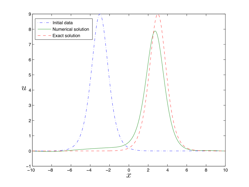
Figure 1. Initial data, and the exact and numerical solutions at $t=2$ with initial data $w_{1}(x,-1)$ with $N=1000$ grid points.

We have also computed numerically the error for a range of ${\Delta x}$, where the relative error is defined by

$$E=100\frac{\sum_{j=1}^{N}\left|w_{1}(x_{j},1)-u_{\Delta x}(x_{j},2)\right|}{\sum_{j=1}^{N}w_{1}(x_{j},1)}.$$

Recall that we are using $w_{1}(x,-1)$ as initial data, so that $w_{1}(x,1)$ represents the solution at $t=2$. In Table 1 we show the relative errors as well as the numerical convergence rates for this example.

$N$	$E$	rate
500	51.2
1000	31.4	0.70
2000	17.6	0.83
4000	9.4	0.91
8000	4.9	0.95
16000	2.5	0.96

Table 1. Relative errors for the one-soliton solution.

The numerical convergence rate indicates that, as expected, the scheme is of first order. Note also that we have to use a rather small ${\Delta x}$ in order to get a reasonably small error. Computing soliton solutions is quite hard, since these solutions are close to zero outside a bounded interval, and the speed of the soliton is proportional to its height. Therefore, if a numerical method (due to, e.g., numerical diffusion) does not have the correct height, it will also have a wrong speed. Thus after some time, it will be in the wrong place and the error is close to 100%.

5.2. A two-soliton solution

Another exact solution of (1.1) is the so-called two-soliton,

(5.2) $$w_{2}(x,t)=6(b-a)\frac{b\operatorname*{csch}^{2}\left(\sqrt{b/2}(x-2bt)\right)+a\operatorname*{sech}^{2}\left(\sqrt{a/2}(x-2at)\right)}{\left(\sqrt{a}\tanh\left(\sqrt{a/2}(x-2at)\right)-\sqrt{b}\coth\left(\sqrt{b/2}(x-2bt)\right)\right)^{2}},$$

for any real numbers $a$ and $b$. We have used $a=0.5$ and $b=1$. This solution represents two waves that “collide” at $t=0$ and separate for $t>0$. For large $\left|t\right|$, $w_{2}(\,\cdot\,,t)$ is close to a sum of two one-solitons at different locations.

Computationally, this is a much harder problem than the one-soliton solution. As initial data we have used $u_{0}(x)=w_{2}(x,-10)$. In Figure 2 we show the exact and numerical solutions at $t=20$.

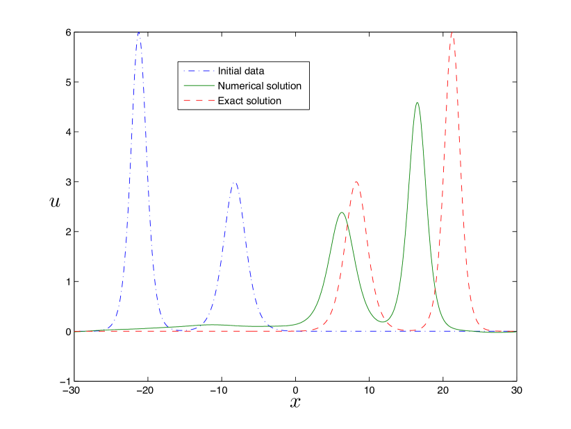
Figure 2. Initial data, and the exact and numerical solutions at $t=20$ with initial data $w_{2}(x,-10)$ with $N=4000$ grid points.

Although we have used 4000 grid points, the error is a staggering 140%! We see that the qualitative features are “right”, in the sense that the larger soliton has overtaken the slower one, but neither their heights nor their positions are correct. For sufficiently small ${\Delta x}$, the numerical solution will be close to the exact also in this case, but it is impractical to calculate numerical convergence rates since the computations would take too much time.

5.3. Initial data in $L^{2}$

We have also tried our scheme on an example where the initial data is in $L^{2}$, but not in any Sobolev space with positive index. Furthermore, note that all the conclusions in Section 4 remain valid if we restrict ourselves to the periodic case. Therefore we have chosen initial data

(5.3) $$u_{0}(x)=\begin{cases}0&x\leq 0,\\ x^{-1/3}&0<x<1,\\ 0&x\geq 1,\end{cases}$$

if $x$ is in $[-5,5]$, and extended it periodically outside this interval. In this case we have no exact solution available. Therefore we can only determine the convergence by viewing solutions with different ${\Delta x}$. In Figure 3 we have plotted the numerical solutions at $t=0.5$ using $3750$, $7500$, $15000$ and $30000$ grid cells in the interval $[-5,5]$.

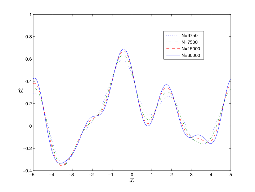
Figure 3. The numerical solution $u_{\Delta x}(x,0.5)$ with initial data (5.3) for various ${\Delta x}$.

From this figure we can observe that the numerical solutions seem to converge nicely to a (smooth) function. The coarser features are already resolved using $3750$ grid cells, and only the finer structures become more apparent for smaller ${\Delta x}$.

Appendix A Sobolev inequalities

For the convenience of the reader we include proofs of the discrete Sobolev inequalities, that are frequently used, but rarely proved.

Lemma A.1.

Given $m_{1},m_{2},m_{3},n_{1},n_{2}\in\mathbb{N}_{0}$, we define $m=m_{1}+m_{2}+m_{3}$ and $n=n_{1}+n_{2}$. Assume $m<n$. Consider $u\in\ell^{2}(\mathbb{R})$. Given a positive $\varepsilon$. The following estimates hold

(A.1) $$\left\|D_{+}^{m_{1}}D_{-}^{m_{2}}D^{m_{3}}u\right\|_{2}^{2} \leq\varepsilon\left\|D_{+}^{n_{1}}D_{-}^{n_{2}}u\right\|_{2}^{2}+C(\varepsilon)\left\|u\right\|_{2}^{2},$$

(A.2) $$\left\|D_{+}^{m_{1}}D_{-}^{m_{2}}D^{m_{3}}u\right\|_{\infty}^{2} \leq\varepsilon\left\|D_{+}^{n_{1}}D_{-}^{n_{2}}u\right\|_{2}^{2}+C(\varepsilon)\left\|u\right\|_{2}^{2},$$

for some function $C(\varepsilon)$.

The same estimates hold in the periodic case where $u\in\ell^{\infty}(\mathbb{R})$ is such that there exists a period $J\in\mathbb{N}$ such that $u_{j+J}=u_{j}$ for all $j\in\mathbb{Z}$, and the norms are taken over the period.

Proof.

We here treat the case of the full line only. Assume first that $m_{3}=0$. The proof follows by induction. Let $m=1$ and $n=2$. Then we have

$$\left\|D_{\pm}u\right\|_{2}^{2} =-(u,D_{+}D_{-}u)$$

$$\leq\varepsilon\left\|D_{+}D_{-}u\right\|_{2}^{2}+C(\varepsilon)\left\|u\right\|_{2}^{2}.$$

Since $\left\|D_{+}D_{-}u\right\|_{2}=\left\|D_{+}^{2}u\right\|_{2}=\left\|D_{-}^{2}u\right\|_{2}$, we have shown (A.1) in the case with $m=1$ and $n=2$. Assume now that (A.1) holds for all cases with $m\leq N$ for some fixed but arbitrary $N$, and all $n=m+1$. Given $m_{1},m_{2},n_{1},n_{2}$ such that $m=m_{1}+m_{2}=N+1$ and $n=n_{1}+n_{2}=m+1$. We then find

$$\left\|D_{+}^{m_{1}}D_{-}^{m_{2}}u\right\|_{2}^{2} =\left|(D_{+}^{n_{1}}D_{-}^{n_{2}}u,D_{+}^{m_{1}-(n_{2}-m_{2})}D_{-}^{m_{2}-(n_{1}-m_{1})}u)\right|$$

$$\leq\varepsilon\left\|D_{+}^{n_{1}}D_{-}^{n_{2}}u\right\|_{2}^{2}+C(\varepsilon)\left\|D_{+}^{m-n_{2}}D_{-}^{m-n_{1}}u\right\|_{2}^{2}$$

$$\leq\varepsilon\left\|D_{+}^{n_{1}}D_{-}^{n_{2}}u\right\|_{2}^{2}+C(\varepsilon)\big{(}\varepsilon_{1}\left\|D_{+}^{m_{1}}D_{-}^{m_{2}}u\right\|_{2}^{2}+C(\varepsilon_{1})\left\|u\right\|_{2}^{2}\big{)},$$

using the induction hypothesis since $m-n_{2}+m-n_{1}=m+(m-n)=N$ and $m=N+1$. We can rewrite this as

$$(1-C(\varepsilon)\varepsilon_{1})\left\|D_{+}^{m_{1}}D_{-}^{m_{2}}u\right\|_{2}^{2}\leq\varepsilon\left\|D_{+}^{n_{1}}D_{-}^{n_{2}}u\right\|_{2}^{2}+C(\varepsilon)C(\varepsilon_{1})\left\|u\right\|_{2}^{2}.$$

Given $\varepsilon$ we choose $\varepsilon_{1}$ such that $C(\varepsilon)\varepsilon_{1}\leq\frac{1}{2}$, which proves the case with $m=N+1$ and $n=m+1$. By induction we have shown (A.1) in all cases where $n=m+1$.

Next we show how to extend this result to $n=m+2$ for arbitrary $m$. The general case of $n>m$ follows similarly. Let now $n_{1},n_{2}$ be such that $n=n_{1}+n_{2}=m+2$. We now have

$$\left\|D_{+}^{m_{1}}D_{-}^{m_{2}}u\right\|_{2}^{2} \leq\varepsilon\left\|D_{+}^{n_{1}-1}D_{-}^{n_{2}}u\right\|_{2}^{2}+C(\varepsilon)\left\|u\right\|_{2}^{2}$$

$$\leq\varepsilon\big{(}\varepsilon_{1}\left\|D_{+}^{n_{1}}D_{-}^{n_{2}}u\right\|_{2}^{2}+C(\varepsilon_{1})\left\|u\right\|_{2}^{2}\big{)}+C(\varepsilon)\left\|u\right\|_{2}^{2}$$

$$=\varepsilon\varepsilon_{1}\left\|D_{+}^{n_{1}}D_{-}^{n_{2}}u\right\|_{2}^{2}+\big{(}\varepsilon C(\varepsilon_{1})+C(\varepsilon)\big{)}\left\|u\right\|_{2}^{2},$$

using first that $n_{1}-1+n_{2}=n-1=m+1$. This proves (A.1) in the general case with $m_{3}=0$.

For an arbitrary $m_{3}\in\mathbb{N}$ we observe that

(A.3) $$D_{+}^{m_{1}}D_{-}^{m_{2}}D^{m_{3}}=2^{-m_{3}}\sum_{k=0}^{m_{3}}\binom{m_{3}}{k}D_{+}^{m_{1}+k}D_{-}^{m_{2}+m_{3}-k}$$

using $D=\frac{1}{2}(D_{+}+D_{-})$, which reduces this case to that with $m_{3}=0$.

Consider now the inequality (A.2). Observe that

$$u_{j}^{2}={\Delta x}\sum_{k=-\infty}^{j-1}D_{+}u^{2}_{k}={\Delta x}\sum_{k=-\infty}^{j-1}(u_{k}+u_{k+1})D_{+}u_{k}$$

which implies that

$$\left\|u\right\|_{\infty}^{2}=\left|\big{(}(u+S^{+}u),D_{+}u\big{)}\right|\leq\varepsilon\left\|D_{+}u\right\|_{2}^{2}+C(\varepsilon)\left\|u\right\|_{2}^{2}=\varepsilon\left\|D_{\pm}u\right\|_{2}^{2}+C(\varepsilon)\left\|u\right\|_{2}^{2}.$$

Thus

$$\left\|D_{+}^{m_{1}}D_{-}^{m_{2}}u\right\|_{\infty}^{2} \leq\varepsilon\left\|D_{+}(D_{+}^{m_{1}}D_{-}^{m_{2}}u)\right\|_{2}^{2}+C(\varepsilon)\left\|D_{+}^{m_{1}}D_{-}^{m_{2}}u\right\|_{2}^{2}$$

$$\leq\varepsilon(\varepsilon_{1}\left\|D_{+}^{n_{1}}D_{-}^{n_{2}}u)\right\|_{2}^{2}+C(\varepsilon_{1})\left\|u\right\|_{2}^{2})$$

$$\quad+C(\varepsilon)(\varepsilon_{1}\left\|D_{+}^{n_{1}}D_{-}^{n_{2}}u\right\|_{2}^{2}+C(\varepsilon_{1})\left\|u\right\|_{2}^{2})$$

$$\leq(\varepsilon+C(\varepsilon))\varepsilon_{1}\left\|D_{+}^{n_{1}}D_{-}^{n_{2}}u\right\|_{2}^{2}+(\varepsilon+C(\varepsilon))C(\varepsilon_{1})\left\|u\right\|_{2}^{2}.$$

(In the rare case that $n_{1}=m_{1}+1$ and $n_{2}=m_{2}$ we do not change the first term.) Given $\varepsilon$ we choose $\varepsilon_{1}$ such that $(\varepsilon+C(\varepsilon))\varepsilon_{1}\leq\varepsilon$. This completes the proof of (A.2).

The proof of (A.2) requires some modifications in the periodic case. Let $m$ be such that $\left|u_{m}\right|=\min_{j=0,\dots,J-1}\left|u_{j}\right|$. For $j>m$ we have

$$u_{j}^{2}=u_{m}^{2}+{\Delta x}\sum_{k=m}^{j-1}D_{+}u_{k}^{2}=u_{m}^{2}+{\Delta x}\sum_{k=m}^{j-1}(u_{k}+u_{k+1})D_{+}u_{k}.$$

Thus

$$\max_{j}\left|u_{j}\right|^{2} \leq\min_{j}\left|u_{j}\right|^{2}+\left|\big{(}(u+u^{+}),D_{+}u\big{)}\right|$$

$$\leq\frac{1}{L}\left\|u\right\|^{2}_{2}+\varepsilon\left\|D_{+}u\right\|_{2}^{2}+\tilde{C}(\varepsilon)\left\|u\right\|_{2}^{2}$$

$$\leq\varepsilon\left\|D_{\pm}u\right\|_{2}^{2}+C(\varepsilon)\left\|u\right\|_{2}^{2}.$$

Here we have used that

$$J{\Delta x}\min_{j}\left|u_{j}\right|^{2}\leq{\Delta x}\sum_{k=0}^{J-1}\left|u_{k}\right|^{2}=\left\|u\right\|_{2}^{2},$$

which implies

$$\min_{j}\left|u_{j}\right|^{2}\leq\frac{1}{L}\left\|u\right\|_{2}^{2},$$

where $L=J{\Delta x}$ remains finite and nonzero as ${\Delta x}\to 0$. ∎

Remark A.2.

We could equally well have written the inequalities (A.1), (A.2) as

(A.4) $$\left\|D_{+}^{m_{1}}D_{-}^{m_{2}}D^{m_{3}}u\right\|_{2} \leq\varepsilon\left\|D_{+}^{n_{1}}D_{-}^{n_{2}}u\right\|_{2}+C(\varepsilon)\left\|u\right\|_{2},$$

(A.5) $$\left\|D_{+}^{m_{1}}D_{-}^{m_{2}}D^{m_{3}}u\right\|_{\infty} \leq\varepsilon\left\|D_{+}^{n_{1}}D_{-}^{n_{2}}u\right\|_{2}+C(\varepsilon)\left\|u\right\|_{2}.$$

Acknowledgments. This paper was initiated during the international research program on Nonlinear Partial Differential Equations at the Centre for Advanced Study at the Norwegian Academy of Science and Letters in Oslo and completed during a stay at ETH in Zürich. Both institutions are thanked for their hospitality.

References

- [1] P. Amorim and M. Figueira. Convergence of a finite difference scheme for the KdV and modified KdV equations with initial data. arXiv:1202.1232v1, (2012).
- [2] D. N. Arnold and R. Winther. A superconvergent finite element method for the Korteweg–de Vries equation. Math. Comp. 38:23–36 (1982).
- [3] U. M. Ascher and R. I. McLachlan. On symplectic and multisymplectic schemes for the KdV equation. J. Sci. Computing 25:83–104 (2005).
- [4] G. A. Baker, V. A. Dougalis, and O. A. Karakashian. Convergence of Galerkin approximations for the Korteweg–de Vries equation. Math. Comp. 40:419–433 (1983).
- [5] J. L. Bona, V. A. Dougalis, and O. A. Karakashian. Fully discrete Galerkin methods for the Korteweg–de Vries equation. Comp. & Math. with Appls. 12A:859–884 (1986).
- [6] J. L. Bona and R. Smith. The initial-value problem for the Korteweg–de Vries equation. Philos. Trans. Roy. Soc. London Ser. A 278:555–601 (1975).
- [7] H. Holden, K. H. Karlsen, and N. H. Risebro. Operator splitting methods for generalized Korteweg–de Vries equations. J. Comput. Phys. 153:203–222 (1999).
- [8] H. Holden, K. H. Karlsen, N. H. Risebro, and T. Tao. Operator splitting for the Korteweg–de Vries equation. Math. Comp. 80:821–846 (2010).
- [9] H. Holden, K. H. Karlsen, T. Karper. Operator splitting for two-dimensional incompressible fluid equations. Math. Comp., to appear.
- [10] H. Holden, K. H. Karlsen, K.-A. Lie, and N. H. Risebro. Splitting for Partial Differential Equations with Rough Solutions. Analysis and Matlab programs. European Math. Soc. Publishing House, Zürich, 2010.
- [11] H. Holden, C. Lubich, and N. H. Risebro. Operator splitting for partial differential equations with Burgers nonlinearity. Math. Comp., to appear.
- [12] A.-K. Kassam and L. N. Trefethen. Fourth-order time-stepping for stiff PDEs. SIAM J. Sci. Comput. 26:1214–1233 (2005).
- [13] T. Kato, On the Cauchy problem for the (generalized) Korteweg–de Vries equation. Studies in Applied Mathematics, Adv. Math. Suppl. Stud., vol. 8, Academic Press, New York, 1983, pp. 93–128.
- [14] F. Linares and G. Ponce. Introduction to Nonlinear Dispersive Equations. Universitext, Springer, 2009.
- [15] F. Z. Nouri and D. M. Sloan. A comparison of Fourier pseudospectral methods for the solution of the Korteweg–de Vries equation. J. Comp. Phys. 83:324–344 (1989).
- [16] A. Sjöberg. On the Korteweg–de Vries equation: Existence and uniqueness. J. Math. Anal. Appl. 29:569–579 (1970).
- [17] T. Tao. Nonlinear Dispersive Equations. Local and Global Analysis. Amer. Math. Soc., Providence, 2006.
- [18] F. Tappert. Numerical solutions of the Korteweg–de Vries equation and its generalizations by the split-step Fourier method. In: (A. C. Newell, editor) Nonlinear Wave Motion, Amer. Math. Soc., Providence, 1974, pp. 215–216.
- [19] R. Winther. A conservative finite element method for the Korteweg–de Vries equation. Math. Comp. 34:23–43 (1980).
- [20] N. J. Zabusky and M. D. Kruskal. Interaction of “solitons” in a collisionless plasma and the recurrence of initial states. Phys. Rev. Lett. 15:240–243 (1965).