Obtaining Maxwell’s equations heuristically

Abstract

Starting from the experimental fact that a moving charge experiences the Lorentz force and applying the fundamental principles of simplicity (first order derivatives only) and linearity (superposition principle), we show that the structure of the microscopic Maxwell equations for the electromagnetic fields can be deduced heuristically by using the transformation properties of the fields under space inversion and time reversal. Using the experimental facts of charge conservation and that electromagnetic waves propagate with the speed of light together with Galileo invariance of the Lorentz force allows us to introduce arbitrary electrodynamic units naturally.

I Introduction

Teaching an electrodynamics course one is faced with the question of whether one should postulate Maxwell’s equations, as one postulates Newton’s laws in an introductory classical mechanics course, or whether they should be justified from experimental experience (Coulomb’s law, Faraday’s induction law, Ampère’s law and the nonexistence of magnetic monopoles). Depending on the choice made, the didactic approach is then either deductive (axiomatic) or inductive.

Here we give a heuristic derivation of the microscopic Maxwell equations. This derivation is based on the principles of simplicity (lowest order in space and time derivatives), linearity (superposition principle) and the transformation properties of the fields under space inversion, $\vec{r}\to-\vec{r}$, and time reversal, $t\to-t$. The starting point of the derivation is the experimental fact that a (moving) charge feels the Lorentz force. In addition, in order to define electrodynamic units, we use the experimental evidence of charge conservation, the fact that electromagnetic waves propagate at the speed of light $c$ and the requirement of Galileo invariance of the Lorentz force for low velocities.

Several attempts to deduce (“derive”) Maxwell’s equations have been published.Kobe ; Dyson ; Heras1 ; Heras2 The approach that will be presented below is alternative because it does not need another dynamical equation, for example, the time-dependent Schrödinger equation Kobe or Newton’s law Dyson as a starting point. Our derivation may serve as valuable background information for the lecturer in both approaches to teaching electrodynamics. It can be used as an a posteriori justification after the Maxwell equations have been postulated and/or obtained from pure experimental experience.

The presentation is structured as follows: in Sec. II we briefly review the classification of vectors and scalars by their behavior under space inversion and time reversal. In Sec. III we present the deduction of Maxwell’s equations from the principles of simplicity and linearity, with five undetermined multiplicative constants. Three of the five constants are determined in Sec. IV from well-established experimental facts together with the demand of Galileo invariance of the Lorentz force. Fixing the final two constants leads to the natural introduction of three commonly used systems of units in electrodynamics.

II Polar and axial vectors and time reversal properties

In a standard physics curriculum starting with classical mechanics, the necessity of studying electrodynamics can be motivated by the implications of the particle property charge, be it fixed or moving. Experimental evidence shows that the Lorentz force on a test particle with electric charge $q$, moving with velocity $\vec{v}$ is given by

$$\vec{F}=q\,(\vec{E}+\eta\,\vec{v}\times\vec{B}\,).$$ (1)

This equation postulates the existence of a local electric field $\vec{E}(\vec{r},t)$ and a local magnetic induction $\vec{B}(\vec{r},t)$ at the position of the particle $\vec{r}$, generated by all charge carrying, field generating particles except the test particle itself. A particle with the property magnetic charge is not known up to now. Thus the fields are generated only by electric charges with charge density $\rho$ and moving charges with electric current density $\vec{j}$ (see below).

Due to the multiplicative connection of charge and fields in Eq. (1), their units can be chosen arbitrarily. E. g., an arbitrarily defined charge unit $[q]$ fixes the dimension of the electric field $[E]$ and that of the product $[\eta B]$ with again an arbitrary constant $\eta$ which finally defines $[B]$ and thus fixes the relative dimension of both fields.

Of central importance for the following is the fact that the vector character with respect to space inversion, $\vec{r}\to-\vec{r}$, is twofold:Emde ; Jackson ; Norb90

• Vectors $\vec{p}$, that transform according to

  $$\vec{p}\stackrel{{\scriptstyle\vec{r}\to-\vec{r}}}{{\longrightarrow}}\vec{p}~{}^{\prime}=-\vec{p},$$ (2)

  under inversion are called polar vectors (or just vectors).

• Vectors $\vec{a}$, that transform according to

  $$\vec{a}\stackrel{{\scriptstyle\vec{r}\to-\vec{r}}}{{\longrightarrow}}\vec{a}~{}^{\prime}=\vec{a},$$ (3)

  under inversion are called axial vectors (or pseudo vectors). They need a (right) hand rule for their definition.

As an example from classical mechanics, we explicitly depict the transformation properties of position $\vec{r}$, momentum $\vec{p}$ and angular momentum $\vec{L}$ in Fig. 1.

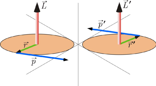
Figure 1: An example for the transformation properties of polar vectors (position $\vec{r}$ and momentum $\vec{p}$) and an axial vector (angular momentum $\vec{L}=\vec{r}\times\vec{p}$) under space inversion wiki .

For the multiplication of different types of vectors the following rules hold:

$$\vec{p}_{1}\times\vec{p}_{2} = \vec{a}$$ (4)

$$\vec{a}_{1}\times\vec{a}_{2} = \vec{a}$$ (5)

$$\vec{a}_{1}\times\vec{p}_{1} = \vec{p}.$$ (6)

Furthermore, in the same manner as there are vectors and pseudo vectors, also scalars $S$ transforming according to

$$S\stackrel{{\scriptstyle\vec{r}\to-\vec{r}}}{{\longrightarrow}}S^{\prime}=S$$ (7)

under inversion and pseudo scalars $S^{\ast}$ with

$$S^{\ast}\stackrel{{\scriptstyle\vec{r}\to-\vec{r}}}{{\longrightarrow}}{S^{\ast}}^{\prime}=-S^{\ast}$$ (8)

can be defined. They can be generated, e. g., by taking the following products

$$\vec{p}_{1}\cdot\vec{p}_{2} = S$$ (9)

$$\vec{a}_{1}\cdot\vec{a}_{2} = S$$ (10)

$$\vec{p}_{1}\cdot\vec{a}_{1} = S^{\ast}$$ (11)

We can now identify the vector, respectively scalar character of the quantities appearing in the Lorentz force, together with their behavior under the reversal of time.

1. Because the mass $m$ is a scalar, $\vec{F}=m\ddot{\vec{r}}$ is a polar vector with $\vec{F}(-t)=\vec{F}(t)$. Therefore, because $q$ in (1) is a scalar, $\vec{E}$ is a polar vector with $\vec{E}(\vec{r},-t)=\vec{E}(\vec{r},t)$.

2. Because the velocity $\vec{v}$ is a polar vector with $\vec{v}(-t)=-\vec{v}(t)$, due to the vector product in (1), $\vec{B}$ is an axial vector with $\vec{B}(\vec{r},-t)=-\vec{B}(\vec{r},t)$.

This unequal nature of the two field vectors of electrodynamics has been known and used in teaching for a long time.foot1 An early appearance and critical discussion in the literature can be found in.Emde

For future reference we state that the field generating charge density is defined by $\varrho:=\lim_{\Delta V\to 0}\Delta Q/\Delta V$, where $\Delta V>0$ because of the discrete nature of charge. Here, as usual, it is idealized as a continuous scalar field with $\varrho(\vec{r},t)=\varrho(-\vec{r},t)$ and $\varrho(\vec{r},-t)=\varrho(\vec{r},t)$ and thus the field generating current density

$$\vec{j}(\vec{r},t)=\varrho(\vec{r},t)~{}\vec{\nu}(\vec{r},t),$$ (12)

with the velocity field $\vec{\nu}(\vec{r},t)$ of the charge density (not to be confused with the test particle velocity $\vec{v}$ in Eq. (1)), is a polar vector with $\vec{j}(\vec{r},t)=-\vec{j}(-\vec{r},t)$ and $\vec{j}(\vec{r},-t)=-\vec{j}(\vec{r},t)$.

III Generating the Maxwell equations: The basic idea

The classic text book by Jackson Jackson contains a discussion showing that the Maxwell equations do indeed equate quantities with the same transformation behavior under time reversal and space inversion. The idea to be presented here is that this behavior together with the Lorentz force and the heuristic demand for simplicity and linearity allows to deduce the structure of the Maxwell equations. The principles of simplicity and linearity together with the symmetry properties of the fields have already been employed by Migdal Migdal to derive the homogeneous curl equations. The program that we will follow here is to equate field generating quantities $\varrho$ and $\vec{j}$ with derivatives of the fields with respect to time or space up to at most first order, and, so that the fields and the inhomogeneous terms fulfill the superposition principle.foot4

Firstly, as discussed above, there is no experimental evidence of magnetic charges. Thus there do not exist any field generating pseudo scalars and the only pseudo scalar (11) that can be generated by taking first order spatial derivatives of any of the fields, which is $\vec{\nabla}\cdot\vec{B}$, has to vanish and we find

$$\vec{\nabla}\cdot\vec{B}=0.$$ (13)

Nevertheless, magnetic monopoles are a topic of current research, especially because, based on an idea by Dirac, they may explain the discrete nature of the electric charge.Schwinger Furthermore, they may be helpful as a didactic tool.Crawford We note in passing that there is a very simple physical argument for the vanishing divergence of $\vec{B}$: if this divergence would be non-zero, a magnetic induction field $\vec{B}$ proportional to $\vec{r}$ would exist (as is well-known from the electric field case) and the Lorentz force (1) would contain terms proportional to $\dot{\vec{r}}\times\vec{r}$, i. e., terms proportional to the angular momentum that would lead to out of plane acceleration. For a charged particle corresponding trajectories have, however, never been observed in pure magnetic induction fields. Concluding the discussion of (13), we mention that mixed terms of the correct symmetry, as, e. g., $\vec{j}\cdot\dot{\vec{B}}$ in (13) would violate the superposition principlefoot4 .

Secondly, due to the fact that $\dot{\vec{B}}$, as well as according to (6) also $\vec{\nabla}\times\vec{E}$, are the only axial vectors without sign change on time reversal they have to appear in one equation together. A field generating axial vector does not exist and the heuristic demand for simplicity and linearity lead us to the equation

$$\vec{\nabla}\times\vec{E}+\chi\,\dot{\vec{B}}=0$$ (14)

with an undetermined constant $\chi$.

Thirdly, the only scalar that can be generated from first derivatives of the fields without sign change on time reversal is $\vec{\nabla}\cdot\vec{E}$. This quantity must be determined by the only scalar source term $\varrho$ and therefore we can write

$$\vec{\nabla}\cdot\vec{E}=\alpha\,\varrho$$ (15)

with a yet undetermined constant $\alpha$. Again we note that mixed terms of the correct symmetry, as, e. g., $\vec{j}\cdot\dot{\vec{E}}$ in (15) would violate the superposition principlefoot4 , whereas a term proportional to $\ddot{\rho}$ violates the use of maximally first order derivatives.

Finally, the only polar vectors with sign change on time reversal that can be generated from the fields by first order derivatives are $\dot{\vec{E}}$ and $\vec{\nabla}\times\vec{B}$; they therefore appear in one equation together with $\vec{j}$, that reads

$$\vec{\nabla}\times\vec{B}+\kappa\,\dot{\vec{E}}=\beta\,\vec{j},$$ (16)

with the two constants $\kappa,\beta$ still to be determined.

The homogeneous (13,14) as well as the inhomogeneous Maxwell equations (15,16) constructed in this way still contain 4 undetermined constants $\chi,\alpha,\kappa$, and $\beta$. Together with the constant $\eta$ appearing in the Lorentz force, Eq. (1), 5 constants still have to be determined.

IV Determining the constants and choice of units

As an experimental fact, the field generating quantities $\rho$ and $\vec{j}$ have to fulfill the equation of continuity. In addition we know that the Lorentz force has to be invariant under Galileo transformation for small $v\ll c$ with the speed of light $c$ (Lorentz invariance adds corrections proportional to $(v/c)^{2}$). Furthermore, from experimental evidence as well as from the theory of special relativity, we know that the universal propagation speed $c$ has to be contained in the wave equation, which can be deduced from the equations obtained in Sec. III (see below). For the five constants we therefore have 3 equations, meaning that there is a degree of ambiguity, which will be resolved by the discussion of three possible, frequently used systems of units, the “Système International d’ unités” (SI units), the Gaussian system (cgs units), and the Heaviside-Lorentz units.

IV.1 Charge conservation

Taking the divergence of (16) together with (15) leads to

$$\beta\vec{\nabla}\cdot\vec{j}=\kappa\,\vec{\nabla}\cdot\dot{\vec{E}}=\kappa\,\alpha\,\dot{\varrho}.$$ (17)

Thus the fundamental equation of continuity $\dot{\varrho}+\vec{\nabla}\cdot\vec{j}=0$ is fulfilled if

$$\kappa\alpha=-\beta.$$ (18)

IV.2 Invariance of the Lorentz force

The Lorentz invariance of the Lorentz force for small velocities, $v\ll c$, in leading order means Galileo invariance. For the purposes of determining the constant $\chi$ it is therefore sufficient to consider the Galileo transformation $\;\vec{r}\to\vec{r}\,^{\prime}=\vec{r}-\vec{v}_{0}t$; $\;\;\vec{v}\,^{\prime}=\vec{v}-\vec{v}_{0}$. Applied to (1) this leads to

$$\vec{F}=q(\vec{E}+\eta\vec{v}\times\vec{B}\,)=q(\vec{E}+\eta\vec{v}_{0}\times\vec{B}+\eta\vec{v}\,^{\prime}\times\vec{B}\,)\stackrel{{\scriptstyle!}}{{=}}q(\vec{E}\,^{\prime}+\eta\vec{v}\,^{\prime}\times\vec{B}\,^{\prime}).$$ (19)

For the fields, the postulated invariance of the Lorentz force means

$$\vec{E}\,^{\prime}=\vec{E}+\eta\vec{v}_{0}\times\vec{B}\,,\quad\vec{B}\,^{\prime}=\vec{B}.$$ (20)

Using a calculation similar to that in,Jammer we find on the other hand

$$\frac{\partial}{\partial\vec{r}}\times\vec{E}(\vec{r},t) = \frac{\partial}{\partial\vec{r}\,^{\prime}}\times\vec{E}(\vec{r}\,^{\prime}+\vec{v}_{0}t,t)$$ (21)

$$\left.\frac{\partial\vec{B}(\vec{r},t)}{\partial t}\right|_{\vec{r}=\mbox{\tiny const}} = \left.\frac{\partial\vec{B}(\vec{r}\,^{\prime}+\vec{v}_{0}t,t)}{\partial t}\right|_{\vec{r}\,^{\prime}=\mbox{\tiny const}}-\left(\vec{v}_{0}\cdot\frac{\partial}{\partial\vec{r}\,^{\prime}}\right)\vec{B}$$ (22)

$$= \left.\frac{\partial\vec{B}(\vec{r}\,^{\prime}+\vec{v}_{0}t,t)}{\partial t}\right|_{\vec{r}\,^{\prime}}+\frac{\partial}{\partial\vec{r}\,^{\prime}}\times\left(\vec{v}_{0}\times\vec{B}\,\right).$$ (23)

For (14) this leads to

$$\frac{\partial}{\partial\vec{r}}\times\vec{E}+\chi\dot{\vec{B}}=\frac{\partial}{\partial\vec{r}\,^{\prime}}\times\left(\vec{E}+\chi\vec{v}_{0}\times\vec{B}\,\right)+\chi\left.\frac{\partial\vec{B}}{\partial t}\right|_{\vec{r}\,^{\prime}}\stackrel{{\scriptstyle!}}{{=}}\frac{\partial}{\partial\vec{r}\,^{\prime}}\times\vec{E}\,^{\prime}+\chi\frac{\partial\vec{B}\,^{\prime}}{\partial t}=0.$$ (24)

Therefore

$$\vec{E}\,^{\prime}=\vec{E}+\chi\vec{v}_{0}\times\vec{B}$$ (25)

has to hold and by comparison with (20) we find

$$\chi=\eta.$$ (26)

IV.3 Wave equation

The wave equation for vanishing inhomogeneities $\varrho$ and $\vec{j}$ follows by taking the curl of (14) and using (15) and (16). With $\vec{\nabla}\times(\vec{\nabla}\times\vec{E})=\vec{\nabla}(\vec{\nabla}\cdot\vec{E}\,)-\Delta\vec{E}$ this leads to

$$\vec{\nabla}(\vec{\nabla}\cdot\vec{E}\,)-\Delta\vec{E}+\chi\,\vec{\nabla}\times\dot{\vec{B}}=-\Delta\vec{E}-\chi\kappa\,\ddot{\vec{E}}=0.$$ (27)

Finally, using (26) we find that

$$\eta\kappa=-\frac{1}{c^{2}}$$ (28)

has to hold for the remaining constants with a velocity $c$, determined by measuring the velocity of electromagnetic waves in vacuum, which turns out to be $c=$2.9986$\times 10^{8}$m/s, the (universal) vacuum speed of light. It is worthwhile to note that a velocity with the same numerical value can be determined by pure electrostatic and magnetostatic measurements (“$c$ equivalence principle”).Heras3 ; Heras4

IV.4 Final choice of the system of units

The constant $\chi$ is now fixed by (26) and for $\kappa,\alpha,\beta$, and $\eta$ we have the two relations (18) and (28), leading to $\alpha/(\eta\beta)=c^{2}$.Heras1 Two of the constants can be chosen arbitrarily. Common choices are:

• SI units: $\eta=1$ leading to $\kappa=-1/c^{2}$, and $\beta=4\pi\times 10^{-7}$N/A${}^{2}\equiv\mu_{0}$ leading to $\alpha=\mu_{0}c^{2}\equiv 1/\varepsilon_{0}$ and thus to the Lorentz force

  $$\vec{F}=q[\vec{E}(\vec{r},t)+\vec{v}\times\vec{B}(\vec{r},t)],$$ (29)

  and the rationalized Maxwell equations (without explicit appearance of $\pi$)

  $$\vec{\nabla}\times\vec{E}(\vec{r},t) = -\dot{\vec{B}}(\vec{r},t)$$ (30)

  $$\vec{\nabla}\times\vec{B}(\vec{r},t) = \mu_{0}\vec{j}(\vec{r},t)+\mu_{0}\varepsilon_{0}\dot{\vec{E}}(\vec{r},t)$$ (31)

  $$\vec{\nabla}\cdot\vec{E}(\vec{r},t) = \frac{\varrho(\vec{r},t)}{\varepsilon_{0}}$$ (32)

  $$\vec{\nabla}\cdot\vec{B}(\vec{r},t) = 0.$$ (33)

• cgs units: $\eta=1/c$ leading to $\kappa=-1/c$, and $\beta=4\pi/c$ leading to $\alpha=4\pi$, and the Lorentz force

  $$\vec{F}=q[\vec{E}(\vec{r},t)+\frac{\vec{v}}{c}\times\vec{B}(\vec{r},t)],$$ (34)

  where the electric field and the magnetic induction have the same units. The Maxwell equations read

  $$\vec{\nabla}\times\vec{E}(\vec{r},t) = -\frac{1}{c}\dot{\vec{B}}(\vec{r},t)$$ (35)

  $$\vec{\nabla}\times\vec{B}(\vec{r},t) = \frac{4\pi}{c}\vec{j}(\vec{r},t)+\frac{1}{c}\dot{\vec{E}}(\vec{r},t)$$ (36)

  $$\vec{\nabla}\cdot\vec{E}(\vec{r},t) = 4\pi\varrho(\vec{r},t)$$ (37)

  $$\vec{\nabla}\cdot\vec{B}(\vec{r},t) = 0.$$ (38)

• Heaviside-Lorentz units: $\eta=1/c$ leading to $\kappa=-1/c$, and $\beta=1/c$ leading to $\alpha=1$. This gives again the Lorentz force (34) from above but with different field units (although electric field $\vec{E}$ and magnetic induction $\vec{B}$ have again the same units) and leads to rationalized Maxwell equations, but without the explicit appearance of $\varepsilon_{0}$ and $\mu_{0}$

  $$\vec{\nabla}\times\vec{E}(\vec{r},t) = -\frac{1}{c}\dot{\vec{B}}(\vec{r},t)$$ (39)

  $$\vec{\nabla}\times\vec{B}(\vec{r},t) = \frac{1}{c}\vec{j}(\vec{r},t)+\frac{1}{c}\dot{\vec{E}}(\vec{r},t)$$ (40)

  $$\vec{\nabla}\cdot\vec{E}(\vec{r},t) = \varrho(\vec{r},t)$$ (41)

  $$\vec{\nabla}\cdot\vec{B}(\vec{r},t) = 0.$$ (42)

In this way the units are introduced naturally by fixing two remaining constants appearing in the Maxwell equations and the Lorentz force.

V Summary

Starting from the Lorentz force as an experimental fact and using the principles of simplicity and linearity, we could show that the structure of the Maxwell equations for the electromagnetic fields in vacuum can be deduced. These are two (pseudo)scalar equations for the divergence of the respective fields and two (pseudo)vector equations for the curl of the fields, in accord with the fundamental theorem of vector calculus. The vector character (polar or axial) of the fields and their transformation properties under time reversal are at the heart of our presented approach. Charge conservation, the Galileo invariance of the Lorentz force and the fact that electromagnetic waves propagate at the speed of light enabled us to fix three of the five undetermined constants in the Lorentz force and the 4 deduced Maxwell equations. As an additional useful result of the calculation, arbitrary systems of units can be introduced, which is didactically more pleasing than to postulate the units a priori.

^† deceased on August 17, 2009

References

- (1) Donald H. Kobe, “Derivation of Maxwell’s equations from the local gauge invariance of quantum mechanics”, Am J. Phys. 46, 342-348 (1978).
- (2) Freeman J. Dyson, “Feynman’s proof of the Maxwell equations”, Am. J. Phys. 58, 209-211 (1990).
- (3) José A. Heras, “Can Maxwell’s equations be obtained from the continuity equation?”, Am. J. Phys. 75, 652-657 (2007).
- (4) José A. Heras, “How to obtain the covariant form of Maxwell’s equations from the continuity equation”, Eur. J. Phys. 30, 845-854 (2009).
- (5) Fritz Emde, “Polare und axiale Vektoren in der Physik”, Z. Phys. A 12, 258-264 (1923).
- (6) John David Jackson, Classical Electrodynamics, 2nd. ed. (Wiley, New York, 1975).
- (7) J. W. Norbury, “The invariance of classical electromagnetism under charge conjugation, parity and time reversal (CPT) transformations”, Eur. J. Phys. 11, 99-102 (1990).
- (8) adapted from http://commons.wikimedia.org/wiki/File:Angular_momentum_circle.png
- (9) The different nature of and is apparent also in the construction of the electromagnetic field tensor in the covariant formulation of electrodynamics.
- (10) Arkadi B. Migdal, Qualitative Methods in Quantum Theory (Benjamin, Reading MA, 1977).
- (11) The superposition principle for an inhomogeneous, partial differential equation, with linear differential operator states that with two solutions obeying and also the sum is a solution for the inhomogeneity .
- (12) Julian Schwinger, “A Magnetic Model of Matter”, Science 165, 757-761 (1969).
- (13) Frank S. Crawford, “Magnetic monopoles, Galilean invariance, and Maxwell’s equations”, Am. J. Phys. 60, 109-114 (1992).
- (14) Max Jammer and John Stachel, “If Maxwell has worked between Ampère and Faraday: An historical fable with a pedagogical moral”, Am. J. Phys. 48, 5-7 (1980).
- (15) José A. Heras, “The Galilean limits of Maxwell’s equations”, Am. J. Phys. 78, 1048-1055 (2010).
- (16) José A. Heras, “The equivalence principle and the correct form of writing Maxwell’s equations”, Eur. J. Phys. 31, 1177-1185 (2010).