Submillimetre line spectrum of the Seyfert galaxy NGC 1068 from the Herschel-SPIRE Fourier Transform Spectrometer

Abstract

The first complete submillimetre spectrum (190-670$\mu$m) of the Seyfert 2 galaxy NGC 1068 has been observed with the SPIRE Fourier Transform Spectrometer onboard the Herschel Space Observatory. The sequence of CO lines (J_up=4-13), lines from H₂O, the fundamental rotational transition of HF, two o-H₂O⁺ lines and one line each from CH⁺ and OH⁺ have been detected, together with the two [CI] lines and the [NII]205$\mu$m line. The observations in both single pointing mode with sparse image sampling and in mapping mode with full image sampling allow us to disentangle two molecular emission components, one due to the compact circum-nuclear disk (CND) and one from the extended region encompassing the star forming ring (SF-ring). Radiative transfer models show that the two CO components are characterized by density of $n({\rm H_{2}})$=$10^{4.5}$ and $10^{2.9}$ cm^-3 and temperature of $T_{\rm kin}$ =100K and 127K, respectively. The comparison of the CO line intensities with photodissociation region (PDR) and X-ray dominated region (XDR) models, together with other observational constraints, such as the observed CO surface brightness and the radiation field, indicate that the best explanation for the CO excitation of the CND is an XDR with density of n(H₂) $\sim$ 10⁴ cm^-3 and X-ray flux of 9 erg s^-1 cm^-2, consistent with illumination by the active galactic nucleus, while the CO lines in the SF-ring are better modeled by a PDR. The detected water transitions, together with those observed with the Herschel  PACS Spectrometer, can be modeled by an LVG model with low temperature ($T_{\rm kin}\sim$ 40K) and high density ($n({\rm H_{2}})$ in the range $10^{6.7}$ — $10^{7.9}$ cm^-3). The emission of H₂O⁺ and OH⁺ are in agreement with PDR models with cosmic ray ionization. The diffuse ionized atomic component observed through the [NII]205$\mu$m line is consistent with previous photoionization models of the starburst.

1. Introduction

NGC 1068 (Messier 77) is a nearby ($cz$ = 1137 km s^-1) and bright (L_IR=L_8-1000μm $\sim$2 $\times$ 10¹¹ L_⊙, Bland-Hawthorn et al. 1997) Seyfert galaxy, often considered as the prototypical Seyfert type 2 galaxy. However, since the discovery of the broad permitted lines in the polarized optical spectrum of NGC 1068 (Antonucci & Miller, 1985), it has become clear that this galaxy was in reality a hidden broad line region galaxy. The general distinction between the two types of Seyfert galaxies might be due only to orientation effects, according to the so called Unification model (Antonucci, 1993).

Being the strongest nearby Seyfert 2 galaxy, it has been observed extensively over the whole electromagnetic spectrum. Molecular (CO and HCN) observations have shown a prominent starburst ring (hereafter SF-ring) at a radius of 1.0-1.5 kpc and a central circum-nuclear disk (hereafter CND) with a diameter of $d$ $\sim$ 300 pc (Tacconi et al., 1994; Schinnerer et al., 2000). Near-IR observations (Scoville et al., 1988; Thronson et al., 1989) have clearly revealed a 2.3 kpc stellar bar. The compact ($\sim$1 pc) hot dust source in the nucleus of NGC 1068, measured using near-infrared speckle imaging and integral field spectroscopy (Thatte et al., 1997), is probably heated by the AGN’s strong radiation field and possibly associated with the postulated dense circum-nuclear torus. A jet was observed from centimeter to millimeter wavelengths extending out to several kiloparsecs from the center (e.g., Krips et al., 2006; Gallimore et al., 2004). Mid-IR observations revealed hot and ionized gas biconically following the path of the radio jet (e.g., Müller Sánchez et al., 2009, and references therein) and indicating the existence of a parsec-scale warm dust torus (Jaffe et al., 2004). Recent interferometric observations of CO (3-2) and CO (1-0) show that the CO (3-2) emission peaks in the central region within $\sim$ 5 $\arcsec$ from the nucleus, while the CO(1-0) emission is mainly located along the spiral arms (Tsai et al., 2012).

Spectroscopic coverage of NGC 1068 has been extensive. In the mid-IR to far-IR wavelength range, spectra have been measured by the ISO (Kessler et al., 1996) SWS (de Graauw et al., 1996) and LWS (Clegg et al., 1996) spectrometers (Lutz et al., 2000; Spinoglio et al., 2005, respectively), covering the 2.4-45 $\mu$m and 43-197 $\mu$m spectral ranges. At millimeter wavelengths it was recently observed from the ground in the 190-307 GHz (976-1578 $\mu$m) range (Kamenetzky et al., 2011). The submillimeter waveband is one of the few spectral regions that have not been so far explored; the new observations made by the Spectral and Photometric Imaging Receiver (SPIRE) (Griffin et al., 2010) Fourier Transform Spectrometer (FTS) (Naylor et al., 2010b), onboard the Herschel Space Observatory (Pilbratt et al., 2010), covering the spectral range from 190 $\mu$m to 670 $\mu$m, fill most of this gap with the first complete submillimeter spectrum of NGC 1068.

Submillimeter spectral measurements are of particular interest as NGC 1068 is a prime candidate to study the effects of the AGN onto the circum-nuclear material and the surrounding disk. In particular, the study of the excitation conditions and chemistry of the CND appear already from the existing ground-based molecular line observations to be very different from the starburst galaxies environments. The peculiar line ratios of different molecular transitions, mostly HCN, HCO⁺, and ¹²CO, led to the suggestion that the CND of NGC 1068 harbors a giant X-ray-dominated region (XDR, e.g., Rotaciuc et al., 1991; Maloney et al., 1996; Usero et al., 2004; Kohno et al., 2008). The HCN and HCO⁺ molecular line studies of Krips et al. (2008, 2011) confirm an increased abundance of HCN and/or increased kinetic temperatures. CO lines can also discriminate between “classical” photodissociation regions (PDRs) and X-ray dominated regions (XDRs) (e.g. Meijerink & Spaans, 2005). Using the intermediate J rotational lines from the CO molecule, from J_up=4 to J_up=13, which can be observed with the SPIRE FTS, we want to test if indeed in NGC 1068 an XDR is needed to explain the spectral line energy distribution originating from the CND. The case of the ultraluminous IR galaxy Mrk231 already demonstrated that the Herschel-SPIRE data are indeed able to discriminate between the two emission mechanisms and therefore detect the effects of the AGN (van der Werf et al., 2010). Herschel-PACS observations of the high-J CO lines (J${}_{up}\geq 14$) detected in NGC 1068 have been recently presented by Hailey-Dunsheath et al. (2012). The two components, at high and medium excitation, needed to explain the observed CO lines arising from the central 10$\arcsec$ region from J_up= 14 to J_up= 24 can be excited by X-ray or shock heating, while far-UV heating is unlikely.

The Herschel-SPIRE spectroscopic observations of NGC 1068 presented here have been collected under the guaranteed time key project “Physical Processes in the Interstellar Medium of Very Nearby Galaxies” (PI: Christine Wilson). Within the same observational program, SPIRE and Photodetector Array Camera and Spectrometer (PACS) (Poglitsch et al., 2010) photometric images have been collected, which will be presented in a forthcoming paper with the detailed analysis of the continuum emission (Spinoglio et al 2012, in prep.).

2. Observations

2.1. SPIRE Spectroscopy

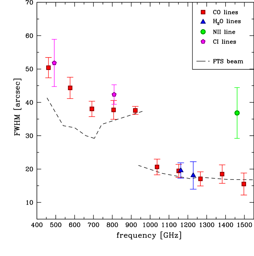
Figure 1.— Observed source sizes, as measured from the mapping observations of the brightest SPIRE lines (FWHM in arcsec, with 1$\sigma$ error bars) as a function of frequency (colored points) compared with the SPIRE-FTS beam (broken lines). All source sizes in the SSW, except for [NII]205 $\mu$m, are consistent with the beam width at that frequency. In contrast, the source sizes in the SLW are more extended than the beam.

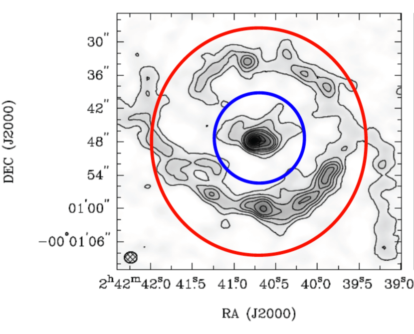
Figure 2.— Left: CO(3-2) integrated intensity map of the central region of NGC 1068 from Tsai et al. (2012). Right: CO(1-0) integrated intensity map of the central region of NGC 1068 from Tsai et al. (2012). The minimum SSW (blue) and the maximum SLW (red) SPIRE FTS beam sizes of 17$\arcsec$ and 42$\arcsec$, respectively, are shown in the figures as concentric circles.

NGC 1068 was observed with the SPIRE-FTS (Griffin et al., 2010) onboard the Herschel Space Observatory (Pilbratt et al., 2010) both in the single pointing mode with sparse image sampling and in the mapping mode with full image sampling. The FTS has two detectors arrays called the spectrometer long wave (SLW, in the range of 303-671 $\mu$m) and the spectrometer short wave (SSW, in the range 194-313 $\mu$m), with a small (10 $\mu$m) overlap in wavelength. The spectral resolution of the FTS ranges from about 280 km s^-1 to 950 km s^-1 in the high resolution mode, moving in wavelength from 194 $\mu$m to 671 $\mu$m. The two SPIRE FTS observations of NGC 1068 were collected on Operational Day 626 (29 January 2011); the fully sampled map has Observation ID 1342213444 and the single pointing ”deep” spectrum has Observation ID 1342213445. The pointed observations were carried out both at low and high spectral resolutions (FWHM $\sim$ 30 GHz and 1.44 GHz), covered with 32 repetitions each, for a total on-source integration time of 410 seconds and 4,262 seconds respectively. The shallower mapping observations at high resolution had 8 repetitions and covered an area with a diameter of approximately 2$\arcmin$. The total on-source integration time was 17,050 seconds.

The FTS beam size and shape vary as a function of frequency and cannot be characterized by a simple Gaussian response. As can be seen from Figure 1, where the observed source sizes of the brightest lines detected by the mapping observations of the SPIRE FTS are plotted as a function of frequency (see the method described in Section 2.1.1), the FTS beam widths (FWHM) range from 17″ to 42″, probing a wider area in the sky with increasing wavelength, and show a strong discontinuity between the SLW and SSW bands, due to the multi-moded feed-horns used for the spectrometer arrays (see Section 4.2.3 and Figure 5.13 in the SPIRE Observers’ Manual).

The combination of the complex morphology of the inner region of NGC 1068 with the SPIRE-FTS beam properties yield a particular coupling effect between the two. Figure 2 shows the CO(3-2) and CO(1-0) interferometric maps from Tsai et al. (2012) of the central region of NGC 1068. As can be seen from these maps, the morphology of NGC 1068 is dominated by two main components (see also, e.g., García-Burillo et al., 2010, and references therein): the compact (of the order of 4″ in diameter) CND at the center of the galaxy, possibly associated with the active nucleus, and a relatively extended ring, with a radius of the order of 10-20″, whose emission is dominated by star formation (SF) activity. The relative contribution from these two spatial components to the various rotational transitions of the ¹²CO molecule strongly varies with the transition from the low-J (J${}_{up}\sim 4$) to the high-J (J${}_{up}\sim 13$) lines. In this range the dominant source of CO excitation changes from the extended SF-ring to the compact CND. There is also a variation of the angular scale probed by the FTS beam, from extended (beam FWHM $\sim$ 42″) to compact (17″), as shown by the two concentric circles in the maps of Figure 2.

Figure 3.— The observed submillimeter spectrum of NGC 1068, as measured from the SPIRE-FTS pointed observations. As can be seen the two SSW and SLW spectra do not overlap. This is due to both the different beam sizes and the intrinsically different source sizes.

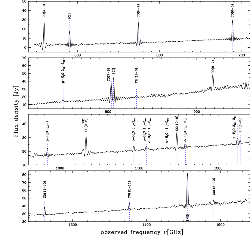
Figure 4.— The observed submillimetre spectrum of NGC 1068, as measured from the SPIRE-FTS pointed observations. From top to bottom are presented the consecutive spectral ranges. The emission line positions are indicated. Line identifications are given for detections with S/N$>$3$\sigma$ (see Table Submillimetre line spectrum of the Seyfert galaxy NGC 1068 from the Herschel-SPIRE Fourier Transform Spectrometer ).

2.1.1 Source size measurements

We first describe the reduction procedure that was used for source size measurements, while in Sections 2.1.2 and 2.1.3 we describe the reduction procedure for spectral line measurements. We employ two reductions as the two measurements have different requirements.

The mapping observations of NGC 1068 have been reduced with the standard reprocessing pipeline in HIPE v.7 and converted into spectral cubes using the NaiveProjection task with custom pixel sizes of 11″  and 13.8″  for the SSW and SLW bands, respectively. These sizes were chosen empirically starting from a large size and reducing it until holes (pixel with zero coverage) appeared in the maps. The final cube for each of the two FTS bands has a variable on-source integration time in the map, between 16 and 32 FTS scans. From these two cubes a number of sub-cubes have been obtained by extracting a 60 GHz wide window (corresponding to $\sim 200$ bins in high spectral resolution) around each line detected in the spectrum of the brightest spaxel, where a spaxel is defined as each one of the 5x5 spatial pixels which fill the spectrometer field of view, and modeling and subtracting the continuum emission with a 1^st order polynomial using HIPE’s task LineIntensityMap.

The FTS data from a pointed observation have two available calibrations which provide the target’s correct flux for the two extreme cases of an unresolved source and of an extended source that completely and uniformly fills the instrument beam. To determine which calibration to use, we measured the emitting region size for several lines from the analysis of the spectra cubes (see Figure 1).

The source sizes of all the transitions present in the SSW band, with the exception of the [NII]205 $\mu$m line, are consistent with originating from an unresolved source and they are therefore well calibrated in the pointed spectrum using the unresolved source solution. For this reason, we used the line fluxes measured from the pointed spectrum for all the transitions in the SSW band except for the [NII]205 $\mu$m line, for which we have used the mapping observations. ([NII] emission arises from ionized gas and so we may expect some contribution from the SF-ring.) For all the transitions in the SLW band, we measured the source sizes from the mapping observations.

We have obtained line integrated maps with the task IntegrateMapFromCube from the spectral sub-cubes. The integration over the lines has made no use of the fitting functionality inside the task, because of the possible spurious detections observed for spectral features with low signal-to-noise ratios. These line maps have been used to measure the angular extent of the region emitting every detected line using a 2D Gaussian fit. While the instrument PSF is not strictly gaussian, because a large fraction of its light is in wider secondary lobes, this approach is robust enough to quantify the scale size of the emitting region through the fit of the PSF core.

In conclusion, the deep pointed spectrum in the SSW band samples primarily, not exclusively, the lines emitted by the compact source, while the SLW band measures lines emitted by both the compact and the extended structures. This coupling effect between the beam and the target morphology makes it difficult to reconstruct the correct spectral line energy distribution (SLED) for the ¹²CO molecular lines for the CND alone. To overcome these problems, we have combined the information extracted from the pointed spectrum with those derived from the mapping observations.

2.1.2 Spectroscopic mapping observations

The mapping observations of NGC 1068 were again reduced using a modified version of the standard Spectrometer Map pipeline script in the Herschel Interactive Processing Environment (HIPE) v.9, developers build 588 and version 8.1 of the SPIRE calibration context. The standard reduction assumes that the source is extended and uniformly fills the beam. Since our source does not fill the beam, the unique point source flux conversion measured for each bolometers was applied to each of the bolometers in our two arrays. After the point source correction, spectral cubes for the SSW and SLW were created using the spireProjection task with projectionType=”naive” with a custom pixel size of $11^{\prime\prime}$ and $13.8^{\prime\prime}$ respectively as before. This cube was used for all SLW and the [NII]$205\mu$m line intensity measurements.

2.1.3 Pointed observations

The single pointing/sparse observations of NGC 1068 have been reduced using the Spectrometer Single Pointing user pipeline in the Herschel Interactive Processing Environment (HIPE) v.9, developers build 588 and version 8.1 of the SPIRE calibration context. An older version of this pipeline is described in Fulton et al. (2010). The observed submillimeter spectrum of NGC 1068, as measured from the SPIRE-FTS pointed observations, is shown in Figure 3, where the large offset at $\sim 300\mathrm{\mu m}$ is due to the large difference in the beam of the SSW and the SLW spectrometers.

2.2. Line intensities

As explained in the previous section, the transitions measured in the SSW band, except for the [NII]205 $\mu$m line, have been considered spatially unresolved and therefore measured from the pointed/deep spectrum, while, on the contrary, the other partially extended lines have been measured from the mapping observations.

In order to measure the line fluxes of the extended component, the line maps have been convolved with 2D kernels (Bendo et al., 2012) to reach the same beam size at every frequency. The final PSF corresponds to the coarsest angular resolution (FWHM = 42″) reached by the FTS for a ¹²CO line (i.e. the CO (4-3) at 461.04 GHz). The kernels were built using the SPIRE-FTS PSF measurements, dividing the PSF image of the CO (4-3) line by that of each detected line in the Fourier space.

The baseline was removed by first masking all of the spectral lines before fitting a high order polynomial to the remaining continuum. The intensities of the detected lines have been computed with a Levenberg Marquardt fitting procedure using the sinc function model. Table Submillimetre line spectrum of the Seyfert galaxy NGC 1068 from the Herschel-SPIRE Fourier Transform Spectrometer presents, for each detected transition, the rest frequency, the energy of the upper level (in K), the beam FWHM (in arcsec.)(see the SPIRE Observers’ Manual, the intensity value with both the 1$\sigma$ statistical uncertainty and total uncertainty, which include the calibration uncertainty added in quadrature. For the mapping observations, we have adopted a fixed FWHM of 43.4″  for all detected lines. For the pointed observations of the compact source, we have adopted a calibration uncertainty of 10%, while for the mapping observations of the extended source, in addition to the calibration uncertainty, we have also added in quadrature a flat-fielding uncertainty of 7%(see the SPIRE Observers’ Manual). The lines detected with the FTS are not spectrally resolved.

Figure 4 presents the observed spectrum of NGC 1068 with the identifications of all lines detected at S/N$>$3. A total of 24 emission emission lines have been detected with the Herschel-SPIRE FTS: ten lines from CO (from J_up=4 to J_up=13), six lines from H₂O, two from H₂O⁺, one from OH⁺, HF and CH⁺ each, in addition to the three atomic lines (from [NII] and [CI]). The apparent ringing in the spectrum is due to the sinc response of the FTS to each line.

In Table Submillimetre line spectrum of the Seyfert galaxy NGC 1068 from the Herschel-SPIRE Fourier Transform Spectrometer we also included literature measurements, relative to both the compact source and the extended source. In particular, we considered in our analysis the interferometric observations of CO (1-0), (2-1) and (3-2) from Krips et al. (2011), and the water lines from the Herschel-PACS observations (S. Hailey-Dunsheath 2012, private communication) for the compact component, and, for the extended component, CO (2-1) Z-Spec spectrometer observations at the Caltech Submillimeter Observatory (CSO) (Kamenetzky et al., 2011) and James Clerk Maxwell Telescope (JCMT) CO (3-2) observations convolved to the 43.4″beam (C. Wilson 2012, private comm.).

3. Results and discussion

3.1. CO Radiation transfer modeling

To obtain a general solution for the CO physical conditions, we have first used the radiative transfer code RADEX (van der Tak et al., 2007). Then, considering the best possible ranges of the parameters as derived from RADEX, we have also used the PDR and XDR models from Wolfire et al. (2010) and Meijerink & Spaans (2005) and Meijerink et al. (2007), respectively, to provide constraints on the origin of the excitation of the measured lines, and in particular to determine whether there is an influence of the AGN, through its X-ray emission, on the molecular gas in the CND and SF-ring associated with NGC 1068.

3.1.1 RADEX models

RADEX is a non-Local Thermodynamic Equilibrium (LTE) code available from the Leiden Atomic and Molecular Database (LAMDA, Schöier et al., 2005). Under the assumption of a uniform medium, using an escape probability formalism that models the entire emitting region as a single zone, RADEX performs statistical equilibrium calculations involving collisional and radiative processes. We used the collisional rate coefficients with H₂ of Yang et al. (2010). Considering the radiation field from background sources given as input, it computes the molecular level populations in the optically thin limit in the first iteration and the optical depths and the escape probabilities for each line. The interdependence of the molecular level populations and the local radiation field requires that the solution is reached through an iterative method. At each iteration, the code computes new level populations using new optical depth values, until the two converge on a consistent solution. Then the resulting line intensities are given as output.

The input parameters required for RADEX are the background radiation field, the kinetic temperature T_kin, the molecular hydrogen number density n(H₂) (assumed to be the only collision partner), and the ratio between the column density of the molecule and the width of the lines, which is the physically relevant quantity that determines the optical depth.

We used RADEX to create a grid of solutions for the CO transitions spanning wide ranges in T_kin, n(H₂), and N_CO (see Table 2). To compare this grid of models with our CO measurements we used the Bayesian likelihood analysis code (Ward et al., 2003), developed by the Z-Spec Team (Naylor et al., 2010a; Kamenetzky et al., 2011).

Figure 5.— RADEX model fitting for the compact component associated with the CND. Square points (red) represent the PACS data, circle points (blue) depict the FTS deep spectrum data, and the diamond points (grey) show the interferometric observations of the CND (Krips et al., 2011), the dotted line shows the ME model of Hailey-Dunsheath et al. (2012), while the dashed line shows the best fitting configuration of RADEX parameters (see column 4D Max of Table 3). The sum of the two models is shown as a solid line.

Figure 6.— RADEX model fitting for the extended component associated with the SF-ring. Notations as in Figure 5. The crosses (yellow) represent the FTS measurements from the spectral map and the white stars show the ground-based observations of the extended component (Kamenetzky et al. 2011, Wilson 2012, private communication). The dot-dashed line shows the best fitting configuration of RADEX parameters (see column 4D Max of Table 3). The thin solid line is the best model for the CND component. The sum of all models is shown as a thick solid line.

Computing the RADEX models, we have considered both models with and without the inclusion of the local background radiation to be added to the cosmological component of the CMB at 2.73K. To estimate the local background in the far-IR, we have fitted the aperture photometry of the Herschel-PACS and SPIRE maps at 70, 160, 250, 350 and 500 $\mu$m, respectively, that will be presented and discussed in a forthcoming paper (Spinoglio et al. 2012, in prep.). We have used a circular aperture with a diameter of 33$\arcsec$  and a dust emissivity law with $\beta$=2 and we have derived a gray-body temperature of 35 K. In agreement with the higher J-CO line fitting results of Hailey-Dunsheath et al. (2012), we have found that the inclusion of this local background does not change significantly the results of the CO fits that only include the CMB. Therefore we have adopted only the CMB black-body radiation at 2.73 K as background radiation, for both the extended and compact sources.

The presence of several spatial and spectral components in the CO SLED has required a multi-step approach, looking for the best solution of one component at a time and subtracting it from the others. We started by considering the CO SLED of the compact source, composed of the FTS-SSW measurements in combination with the compact interferometric observations. For the high-J (J${}_{\rm up}\geq 14$) PACS data, we used the medium excitation (ME) component LVG model presented by Hailey-Dunsheath et al. (2012), characterized by a density of $10^{5.7}\ {\rm cm^{-3}}$ and a kinetic temperature $T_{kin}=150$ K. The ME model for the J_up $>$ 13 CO lines was subtracted from the observed CND spectrum before attempting to fit the SLED.

In Table 3, the results obtained with the Z-Spec code are summarized. For each of the two models of the CND and SF-ring the following parameters are given: the kinetic temperature of the CO, $T_{\rm kin}$, the molecular hydrogen density, $n({\rm H_{2}})$, the CO column density, $N_{CO}$, the area filling factor, $\Phi_{\rm A}$, the gas pressure, $P$, the beam averaged CO column density, $\langle N_{\rm CO}\rangle$, and the molecular hydrogen mass M(H₂), that has been computed using a CO abundance of $x_{CO}=3\times 10^{-4}$, adopted by the Z-Spec code (Naylor et al., 2010a; Kamenetzky et al., 2011).

For each parameter, the median value, the 1-$\sigma$ interval, the 1D and the 4D maximum values are given. 1D refers to the maximum value of the integrated parameter distribution while 4D refers to the value of that parameter at the best fit solution.

The compact source is unresolved with all the considered instruments and identified with the CND, while the extended source data probe the emission arising from a region of 43.4″  in diameter, compatible with the SF-ring structure. We have obtained the best fit to the CND with RADEX, as can be seen in Figure 5, by fitting the mid-J lines (from J_up = 9 to J_up = 13) together with the low-J lines observed with interferometric techniques, which isolate the CND component, and subtracting the contribution from the medium excitation (ME) component of the LVG model of Hailey-Dunsheath et al. (2012).

The best fit of the SF-ring with RADEX (see Figure 6) was then obtained by subtracting from the observed lines (from J_up = 4 to J_up = 8 with SPIRE and J_up = 3 and 2 with JCMT) the contribution arising from the compact source by summing the mid-J and high-J contributions. As can be seen in Figure 6, the extended source gives a significant contribution to the over-all SLED only for J${}_{up}<$9. To summarize, as can be seen in Table 3, we found that the best fit RADEX model results for the CND give $T_{\rm kin}$=100 K and $n({\rm H_{2}})$= $10^{4.5}$ cm^-3 and for the SF-ring $T_{\rm kin}$=127 K and $n({\rm H_{2}})$= $10^{2.9}$ cm^-3.

3.1.2 PDR and XDR models of the CND component

PDR and XDR models from Wolfire et al. (2010) and from Meijerink & Spaans (2005) and Meijerink et al. (2007) describe the thermal and chemical balance of molecular gas that is exposed to far-ultraviolet (FUV) radiation (6-13.6 eV) and X-rays (1-100 keV), respectively. The codes used to determine the gas conditions in these regions as a function of depth take into consideration elaborate chemical networks and the cooling, heating and chemical processes which are completely determined by the radiation field.

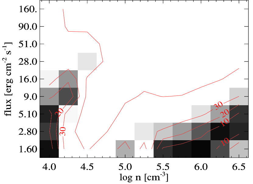
Figure 7.— Reduced $\chi^{2}$ values of the models for the CND. Left: PDR models (Wolfire et al., 2010) ; Right: XDR models (Meijerink & Spaans, 2005; Meijerink et al., 2007).

We have considered the grids of PDR models of Wolfire et al. (2010), that span from 10¹ to 10⁷ cm^-3 in density and from 10^-0.5 to 10^6.5 G₀ in FUV flux. The PDR models are based on those of Kaufman et al. (2006), with updates from Wolfire et al. (2010) and Hollenbach et al. (2012). In particular the atomic and molecular freeze-out and grain chemistry in Hollenbach et al. (2012) are included, as well as their PAH photo rates which affect the ion-neutral chemistry and the production of CO. We use their “linear yield” PAH⁰ photoionization rate slightly modified for a Draine (1978) interstellar radiation field. Hot CO production by HCO⁺ recombinations is also included, as suggested by J. Black (2012, private communication).

For the XDR models, we used the grid by Meijerink et al. (2007) that spans two different ranges in density ($10^{3}-10^{4}\ {\rm cm^{-3}}$ and $10^{4}-10^{6.5}\ {\rm cm^{-3}}$) irradiation ($F_{X}=1.6-160\ {\rm ergs^{-1}cm^{-2}}$), and cloud size of 1 pc and 10 pc. We used a $\chi^{2}$ minimization algorithm to identify the best description of the ¹²CO line fluxes measured with SPIRE and interferometric data (see Table  Submillimetre line spectrum of the Seyfert galaxy NGC 1068 from the Herschel-SPIRE Fourier Transform Spectrometer ).

As already mentioned in Section  3.1.1, in addition to the CO lines detected in NGC 1068 by the SPIRE FTS, presented in Table Submillimetre line spectrum of the Seyfert galaxy NGC 1068 from the Herschel-SPIRE Fourier Transform Spectrometer , higher J lines (from J_up = 14 to J_up = 24) have been observed by PACS and presented in Hailey-Dunsheath et al. (2012). We have tried to model the whole sequence of CO lines detected with PDR/XDR models, however no single component was able to fit the data; three distinct components were needed, all originating from the compact CND, to fit the CO lines down to J_up=9. Moreover, as outlined in Hailey-Dunsheath et al. (2012), even if - in principle - PDR models could fit the data from J_up = 14 to J_up = 24, the morphology of the H₂ near-IR emission and the two different kinematics of the CO lines at J${}_{up}\leq$ 17 and J${}_{up}\geq$ 20, indicate that these two sets of lines trace physically distinct components, therefore excluding a PDR origin of these high-J CO lines. Consequently, for the high-J (J${}_{up}\geq 14$) PACS data we used the model presented by Hailey-Dunsheath et al. (2012), consisting of two XDR components with a density of $10^{5.75}$ cm^-3 and incident X-ray fluxes of 9 and 160 erg s^-1 cm^-2, respectively. Then we have performed the analysis on both the compact source and the extended source, once the other components were fitted and removed as explained in the previous section.

The mid-J lines originating from the CND are best described by a sequence of PDR models ranging from an incident FUV flux of G_o $\sim$ $10^{5.0}$ and density of $10^{4.5}$ cm^-3, in agreement with the RADEX model, to a FUV flux of G_o $\sim$ $10^{2.0}$ and density of $\sim$ $10^{6.0}$ cm^-3 (see left panel of Figure 7). On the other hand, also XDR models either with density $\sim 10^{4.0}$ cm^-3 or $\sim 10^{6.0}$ cm^-3 and incident X-ray flux in the range of 1.6–5.0 erg s^-1 cm^-2 are able to reproduce the observed mid-J CO fluxes with a good $\chi^{2}$ value (see right panel of Figure 7). However, the RADEX models (see section  3.1.1) favor solutions with n_H between $10^{4.4}$ and $10^{4.8}$ cm^-3 as listed in Table 3.

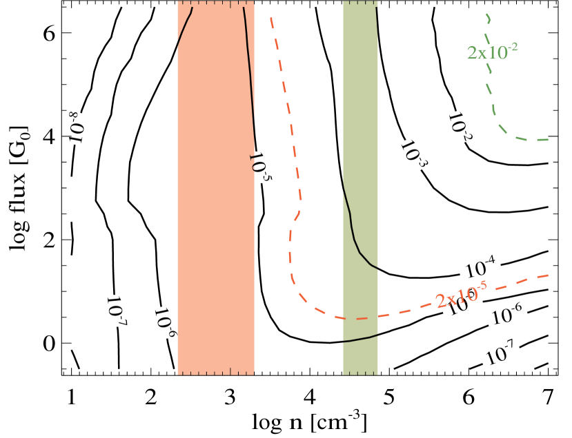
Figure 8.— Total CO surface brightness (in units of erg s^-1 cm^-2 sr^-1) as a function of incident FUV flux and density for the PDR models. The left shaded region (in orange) shows the 1$\sigma$ range of the density of the best fit RADEX model of the SF-ring (extended region), while the right shaded region (in green) reports the area of the 1$\sigma$ range of the density of the best fit RADEX model of the CND (compact component). The red dashed line represents the measured surface density for the SF-ring, while the green dashed line represents the measured surface density for the CND of 0.02 erg s^-1 cm^-2 sr^-1.

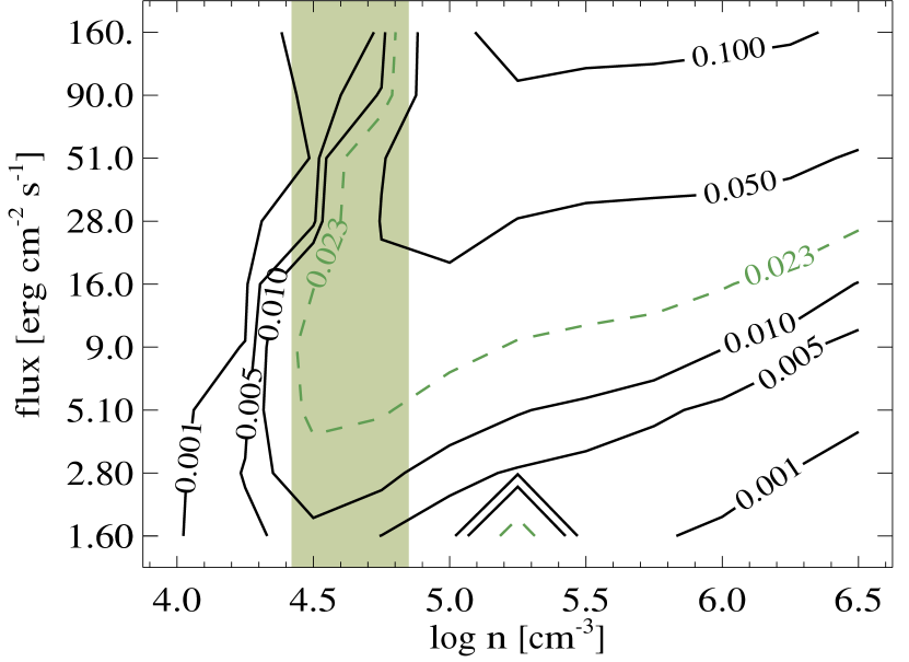
Figure 9.— Total CO surface brightness (in units of erg s^-1 cm^-2 sr^-1) as a function of incident FUV flux and density for the XDR models. The shaded region (in green) shows the 1$\sigma$ range of the density of the best fit RADEX model of the CND (compact component). The dashed line (in green) represents the measured surface density.

To further constrain the models, we have used the CO surface brightness for both PDR and XDR models, by summing over all of the modeled CO lines. For the CND, we have computed the total CO emission from the best fit XDR model presented in Figure  10 and divided by the emitting area of the CND, assumed to be 4 $\arcsec$ in diameter, and corrected by the filling factor of the RADEX best fit (see Table 3) to derive the CO surface brightness of the CND.

In Figures  8 and  9 we present the total CO surface brightness for both PDR and XDR models, respectively, with the density region allowed by the RADEX models indicated by shaded regions. From Figure  8, the predicted CO surface brightness in the CND by PDR models, which satisfies the density constrain of the RADEX model, is about two orders of magnitude below the value computed with the best fit model of the CND of 0.02 erg s^-1 cm^-2 sr^-1. On the other hand, Figure  9 shows that the predicted CO surface brightness in the CND, for an XDR model with density of $\sim$ 10^4.3 cm^-3 and incident X-ray flux $\geq$ 3 erg s^-1 cm^-2, agrees well with the best fit value of 0.02 erg s^-1 cm^-2 sr^-1.

We have also compared the observed parameters of the CND in NGC 1068 with the XDR model results presented for Arp 220 in Rangwala et al. (2011). The XDR model of Arp 220 has been computed using an updated version of the code described by Maloney et al. (1996). The assumed physical conditions in Arp 220 coincide with those of NGC 1068: a hard X-ray (1-100keV) luminosity of L_X $\sim$10⁴⁴erg s^-1, a power law index of $\alpha$ =0.7 and an absorbing hydrogen column density of N_H = 10²⁴ cm^-2, typical of Compton thick sources, like NGC 1068. In their Figure 7 (bottom, right panel), Rangwala et al. (2011) show the predicted CO surface brightness as a function of density and radius of the emitting region. Our best fit value of 0.02 erg s^-1 cm^-2 sr^-1 is in reasonable agreement with a density of $\sim$10⁴ cm^-3 and a radius of 100-200 pc. The radius that we associate to the CO emitting region in the CND is about 160 pc. We therefore conclude that the XDR origin of the CO CND emission in NGC 1068 is indeed a plausible explanation. In Figure  10 we show the fit to the observed CO fluxes using the best fit XDR model with the adopted density and X-ray flux for the CND component.

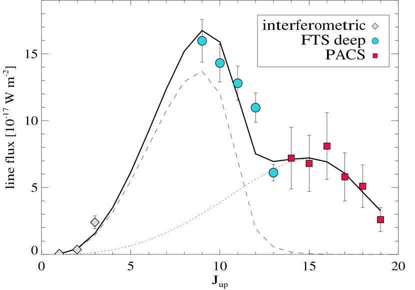
Figure 10.— XDR model fitting for the compact component, associated with the CND. Models have been taken from Meijerink & Spaans (2005) and Meijerink et al. (2007). The points follow the same color code as in Figure 5. The dotted line shows the fit of the high-J CO lines with the XDR model of Hailey-Dunsheath et al. (2012), the dashed lines show the fit of the intermediate-J CO lines, with a XDR model with density $n=10^{4.25}cm^{-3}$ and X-ray flux of 9 erg s^-1 cm^-2, once the high-J CO XDR model has been subtracted. The solid line shows the total modeled emission, which is compared to the observed data (see the text).

3.1.3 PDR and XDR models of the SF-ring component

The low-J component of the SLED can be fitted either by PDR models with a FUV flux of G_o $\gtrsim$ $10^{2}$ and density of $\sim$ $10^{3.5}$ cm^-3, in rough agreement with the RADEX modeling results, or with models with lower FUV flux (G_o $\sim$ $10^{1}$) and a higher density of $\gtrsim$10⁴ cm^-3, which are, however, in conflict with the RADEX results. Moreover (see the right of Figure 11), XDR models with a density $\sim 10^{3.0}$ cm^-3 and incident X-ray flux in the range of 0.5–2.0 erg s^-1 cm^-2 can fit the data.

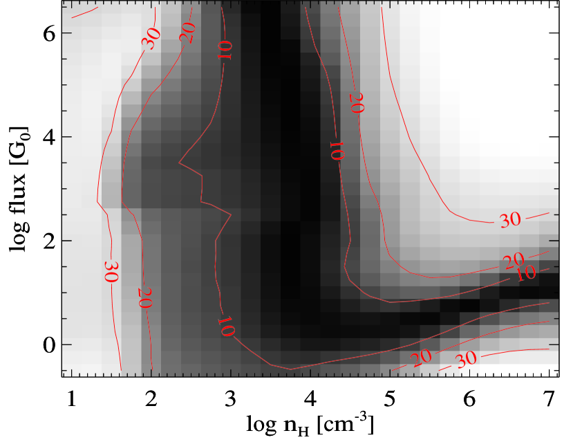
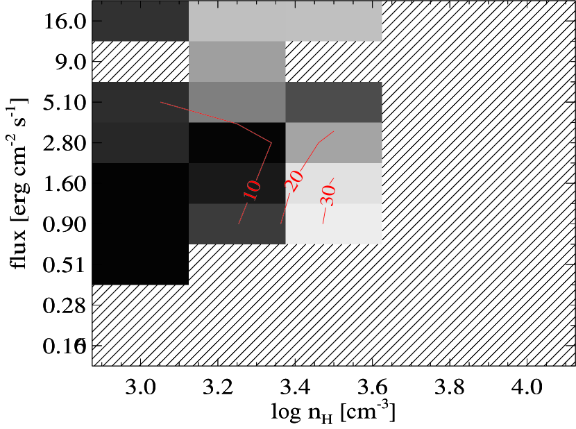
Figure 11.— Reduced $\chi^{2}$ values of the PDR (Wolfire et al., 2010) and XDR models (Meijerink & Spaans, 2005; Meijerink et al., 2007) for the extended component. Left: PDR models; Right: XDR models. The line shaded region of the figure is where no model is available or the model does not predict the lines of interest.

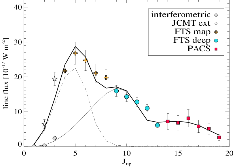
Figure 12.— PDR/XDR model fitting for the extended component (SF-ring), together with the compact component, associated with the CND. Models have been taken from Meijerink & Spaans (2005); Meijerink et al. (2007). Notations as in Figure 6. The crosses (yellow) represent the FTS measurements from the spectral map and the stars (white) show the ground-based observations of the extended component (Kamenetzky et al. 2011, Wilson 2012, private communication). The thin solid lines show the fit of the compact component, which is the sum of the high- and mid-J models as in Figure 10. The dash-dotted lines show the fit of the extended component, with a PDR model with density $n(H_{2})=10^{3.25}cm^{-3}$ and log $Go=2.75$, once the compact component has been subtracted. The thick solid line shows the total modeled emission, which is compared to the observed data (see the text).

Similarly to the case of the CND, described in Section  3.1.2, for the SF-ring we have used the total CO emission from the best fit PDR model and the area of 40$\arcsec$ in diameter to derive the extended component surface brightness. For this latter case, we did not use any filling factor because we consider that the extended emission in the SF-ring is filling most of the beam.

To further constrain the models, we use again the CO surface brightness. From Figure  8, the predicted CO surface brightness in the SF-ring, for a PDR model with density of $\sim$ 10³ cm^-3 and incident FUV flux above $G_{0}\geq 10^{2}$, agrees well with the observed value of $2\times$10^-5 erg s^-1 cm^-2 sr^-1, reinforcing this solution. We present the best fit model in Figure 12.

3.1.4 Constraining the PDR and XDR models with luminosities

In order to verify that the XDR models used to fit the compact (CND) and extended (SF-ring) molecular components in NGC 1068 are in agreement with the intrinsic X-ray flux emitted from the AGN, we have adopted an estimated intrinsic luminosity in the range of L_1-100keV $\sim$ 10⁴³-10^43.5 erg s^-1 (see, e.g. Colbert et al., 2002). Using the diameter of the CND of 4$\arcsec$ and that of the SF-ring of 40$\arcsec$, we derived an X-ray flux in the range of $\sim$ 3-10 erg s^-1cm^-2 and of $\sim$ 0.03-0.11 erg s^-1cm^-2, respectively for the compact and extended components.

The X-ray flux predicted for the XDR model of the CND component is in the range 1.6$<$F_X$<$10 erg s^-1cm^-2 (see right panel of Figure 7), therefore the hypothesis of an XDR origin of the intermediate-J CO lines in the CND can be considered valid. The X-ray flux predicted for the XDR model of the SF-ring of F_X = 0.5–2.0 erg s^-1 cm^-2 is not in agreement with our estimates, being at least one order of magnitude higher, and therefore the XDR origin of the lower-J CO lines in the extended region can be excluded, given the assumption in the above paragraph. Moreover, even if the X-ray flux would be available to excite the XDR, e.g. in the case of an underestimated intrinsic X-ray luminosity, an unknown part of it is expected to be absorbed from the interstellar medium along the path, before reaching the SF-ring. The attenuation to the X-ray source as seen by the CO-emitting gas cannot in fact be quantified. Therefore the estimated flux could be considered as an upper limit.

Similarly we estimated the far-UV (6–13.6 eV) flux from the AGN that illuminates the CND and the SF-ring. The adopted intrinsic far-UV luminosity of the AGN is $\sim$10⁴² erg s^-1. This value was calculated using the intrinsic far-UV continuum derived by Pier et al. (1994). At the distance of the SF-ring the far-UV flux is $F_{\rm FUV}=10^{0.5}$ G₀, whereas for the CND the $F_{\rm FUV}=10^{2.4}$ G₀.

This $F_{\rm FUV}$ for the CND implies a high-density ($n_{\rm H}>10^{5.5}$ cm^-3) component according to the PDR models (left panel of Figure 7), which is not in agreement with the density estimate from the RADEX modeling. For the extended component, the UV flux from the AGN is lower than that predicted by the PDR models; however, in the star-forming ring it is likely that the UV emission from young stars also contributes to the interstellar UV radiation field. For comparison, the far-UV flux from a young stellar cluster (age 5 Myr, see Spinoglio et al. 2005) of stellar mass 10⁴ M_⊙ is 10² G₀ at 50 pc. This far-UV flux is an order of magnitude higher than that from the AGN and would be compatible with the predictions of the PDR models (see left panel of Figure 11).

Taking into account all the above considerations, we therefore conclude that the most plausible explanation for the excitation of the CND is an XDR illuminated from the AGN, while that of the SF-ring is a PDR, mainly excited from the young stellar populations in the galactic arms.

3.2. H₂O emission

We detected 6 H₂O transitions, 2 o-H₂O and 4 p-H₂O lines, above a 3 $\sigma$ level within the SPIRE–FTS spectrum. In Table Submillimetre line spectrum of the Seyfert galaxy NGC 1068 from the Herschel-SPIRE Fourier Transform Spectrometer we list the detected lines, reporting their frequency, upper level energy $E_{\mathrm{up}}/\kappa_{B}$, and the measured flux. We also listed the water lines detected with PACS (S. Hailey-Dunsheath 2012, private communication). The line fluxes detected by PACS were measured with a Gaussian fitting of the line profile of the central spatial pixel (spaxel) and scaling using the standard point-source correction factors. The emission of all H₂O lines detected in the SSW band of the SPIRE-FTS, as well as most of the PACS lines, are unresolved (diameter $\leq 20\arcsec$, for the SPIRE lines, see Figure 1, and $\leq 10\arcsec$, for the PACS lines), indicating that water emission arises mainly from the CND region. Only one line, the p-H₂O $2_{11}-2_{02}$ at 752.033 GHz was observed in the SLW band, with a beam size of $\sim 33.4^{\prime\prime}$, and thus the emission of this transition may have an additional contribution from the starburst ring. However, our maps are not sensitive enough to disentangle the contribution of the starburst ring from the CND. Moreover, the PACS map of the o-H₂O $2_{12}-1_{01}$ line at 179 $\mu$m (1669.905 GHz) shows extended emission (S. Hailey-Dunsheath private communication), most likely associated with the starburst ring. Thus, if there is some contribution from the extended emission in the central spaxel, the measured flux may overestimate the contribution of the nuclear flux.

3.2.1 Excitation analysis

In order to constrain the physical conditions of the water excitation, we built a grid of models using the Large Velocity Gradient (LVG) model in plane parallel geometry described in Ceccarelli et al. (1998) varying the parameters in the following range: $n$(H₂)=10³-10⁸ cm^-3, $T_{kin}=10-1500$ K, $N$(o-H₂O) and $N$(p-H₂O) from 10¹¹ to 10¹⁷ cm^-2. The molecular data were taken from the BASECOL database (Dubernet et al., 2006) and we used the most recent collisional rate coefficients with H₂ (Dubernet et al., 2009; Daniel et al., 2010, 2011), calculated for temperatures between 5 K and 1500 K. The H₂O spectrum has been computed considering 45 levels for the ortho and para water (i.e., considering the levels up to excitation temperatures of $\sim 2000$ K). The two water forms are treated as independent species. We used an ortho-to-para H₂ ratio equal to 1 and an ortho-to-para H₂O ratio of 1. The model includes the effects of the beam filling factor, so it computes the $\chi^{2}$ for each column density minimizing with respect to the source size, temperature, and density. Our model does not include the effects of radiative pumping.

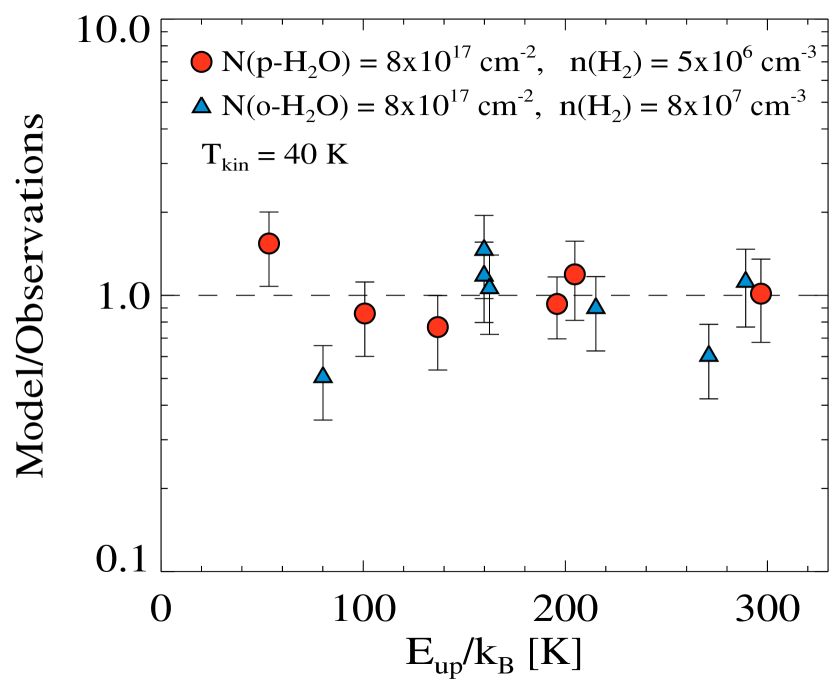
Figure 13.— Ratio between the best fit model predictions and the observations as a function of the upper level energy. Triangles show the o-H₂O transitions and circles show the p-H₂O transitions. The best fit models predict a column density of both ortho- and para-H₂O of $\sim$ 8 $\times$ 10¹⁷ cm^-2 and hydrogen desities in the range n(H₂) = 5 $\times$ 10⁶ - 8 $\times$ 10⁷ cm^-3.

We fitted the o-H₂O and p-H₂O lines separately. We found that the observations of water lines are consistent with LVG model predictions for an emission size of $10^{\prime\prime}\pm 2^{\prime\prime}$, a kinetic temperature of $T_{\mathrm{kin}}$ $\simeq$ 40$\pm$10 K, a density n(H₂) from $4\times 10^{6}$ to $8\times 10^{7}$  cm^-3, and a value of the $N/\Delta\,v$ varying between $5\times 10^{14}$ and $10^{16}$ cm^-2. The column density of each water form can then be obtained once we know the linewidth, which we set to $\sim 100$ km s^-1. This translates into a column density for both o-H₂O and p-H₂O around $5\times 10^{16}-10^{18}$ cm^-2. Figure 13 shows the best fit model for the o-H₂O and p-H₂O lines. The results of the LVG model predictions are summarized in Table 4. As can be seen in Fig. 13, the best fit model predictions can reproduce most of the line fluxes reasonably well. Only for two o-H₂O  lines the LVG model underestimates the observed line flux. However, the line flux of the o-H₂O  2₁₂-1₀₁ transition may be in fact overestimated due to some extended emission that may come from the starburst ring instead from the CND region (S. Hailey-Dunsheath private communication). As shown in previous sections and in Hailey-Dunsheath et al. (2012), the CO emission from the CND is associated with several components at different temperatures and densities. In the case of water we cannot rule out the presence of several components, but, due to the relatively low number of water lines, we did not attempt to fit the water lines with more than one component.

Our results suggest a posteriori that the excitation of the water lines is not strongly affected by radiative pumping. Without the inclusion of radiative pumping, we can indeed fit all the detected lines within a factor of two. Moreover the water transitions in the SPIRE FTS spectrum that should be more affected by radiative pumping, besides that of o-H₂O  3${}_{21}-3_{12}$, are those of o-H₂O  5${}_{23}-5_{14}$ and p-H₂O  4${}_{22}-4_{13}$ (see, e.g., González-Alfonso et al., 2010), which we do not detect, consistent with the LVG model predictions. On the other hand, we compare our findings with the results of Mrk 231 (González-Alfonso et al., 2010), where all these three transitions have been detected and their fluxes can be reproduced only if radiative pumping is included. If we adopt the same line ratios of Mrk 231 for NGC 1068, we would expect to detect also these lines, originating from a higher level, at about a 10$\sigma$ level (assuming the 3$\sigma$ sensitivity in the SSW FTS range of 10^-17 W m^-2). We conclude therefore that for NGC 1068 collisions seem to be the dominant excitation mechanism for water and that radiative pumping can be neglected.

3.3. Molecular ions of H₂O⁺, OH⁺ and CH⁺

The molecular ions of H₂O⁺, OH⁺, and CH⁺ have been detected in emission in NGC 1068. The 1115 GHz ground-state transition of H₂O⁺, as well as the 1033 GHz transition of OH⁺  and that of CH⁺, have also been detected in emission in Mrk 231 (van der Werf et al., 2010). In contrast, these transitions have all been detected in absorption in Arp 220 (Rangwala et al., 2011) and two of them (H₂O⁺  at 1115 GHz and OH⁺  at 1033 GHz) in absorption in M 82 (Kamenetzky et al., 2012).

To obtain the column densities of H₂O⁺, OH⁺, and CH⁺, we assumed that the gas is in local thermodynamical equilibrium (LTE) and the emission is optically thin and originates in the CND region (diameter of 4^′′). Assuming that all levels are populated according to the same excitation temperature, $T_{\mathrm{ex}}$, the column density is given by (see, e.g., Goldsmith & Langer, 1999):

$$N_{\mathrm{mol}}=\frac{4\pi\,F\,Q(T_{\mathrm{ex}})\exp(E_{\mathrm{up}}/k\,T_{\mathrm{ex}})}{h\nu\,A_{\mathrm{ul}}g_{\mathrm{u}}}$$ (1)

where $F$ is the integrated line brightness (in units of erg cm^-2 s^-1 sr^-1), $\nu$ is the frequency of the transition, $E_{\mathrm{up}}$ the energy of the upper level, $Q$($T_{\mathrm{ex}}$) is the partition function at the excitation temperature $T_{\mathrm{ex}}$, and $h$ and $k$ are the Planck and Boltzmann constants, respectively. We approximated the partition function of CH⁺ and OH⁺ to $Q_{\mathrm{rot}}\simeq\,kT_{\mathrm{ex}}/hB$, where $B$ is the rotational constant of the molecule. Einstein coefficients $A_{\mathrm{ul}}$, upper level degeneracy $g_{\mathrm{u}}$, and rotational constants have been obtained from the Cologne Database for Molecular Spectroscopy (CDMS; Müller et al. 2001, 2005). For o-H₂O⁺ the partition function has been obtained using the energy levels listed in the database. Both H₂O⁺ and OH⁺ present hyperfine structure, which is not resolved in the SPIRE FTS spectrum. Therefore, we used $\sum_{i}\,A_{i\mathrm{l}}g_{i}$ to account for the several hyperfine components. We adopted an ortho-to-para ratio for H₂O⁺ of 3.

The estimated column densities are $N$(H₂O⁺)=$(2.0-5.9)\times 10^{13}$ cm^-2, $N$(OH⁺)=$(1.0-1.2)\times 10^{13}$ cm^-2, and $N$(CH⁺)=$(5.4-7.5)\times 10^{13}$ cm^-2, for a range of excitation temperatures between 40 and 100 K. The uncertainty in the derived column densities is estimated to be around 50%, which arises from the uncertainty in the flux calibration. The p-H₃O⁺ $J_{\mathrm{K}}=3_{2}^{+}-2_{2}^{-}$ line at 364.7974 GHz has been detected in NGC 1068 using the JCMT (Aalto et al., 2011). We recomputed the H₃O⁺ column density using Eq. 1, our adopted size of the CND region of $4^{\prime\prime}$, and the excitation temperature range of $T_{\mathrm{ex}}$$\sim 40-100$ K. We obtained $N$(p-H₃O⁺)$\simeq(1.8-0.7)\times 10^{14}$ cm^-2. Assuming an intermediate ortho-to-para ratio of 1.5 (van der Tak et al., 2008), the total column density of H₃O⁺ is $\sim(4.5-1.8)\times 10^{14}$ cm^-2.

Considering the spectrum of Arp 220 presented in Rangwala et al. (2011), we notice that in NGC 1068, the ratio of N(H₃O⁺)/N(H₂O⁺)$\sim$10, whereas this ratio is reversed in Arp 220. Similarly, the inferred column densities indicate that N(H₃O⁺)/N(OH⁺) $\gg$ 1 in NGC 1068, while in Arp 220 the OH⁺ column density is at least an order of magnitude larger than that of H₃O⁺. So the relative abundances of the molecular ions appear to be very different in the two galaxies, suggesting some substantially different conditions.

We compared our estimated column densities with the predictions of the Hollenbach et al. (2012) PDR models for different FUV incident fluxes and cosmic ray ionization rates. For the FUV radiation field produced by the AGN in the CND region (see Section 3.1.4) the order of magnitude of the observed column densities of H₂O⁺ and OH⁺ are compatible with a low density medium (see Fig. 9 and Fig. 10 of Hollenbach et al. (2012)). According to their models, the column density of H₃O⁺ is approximately constant with a value of $10^{14}$ cm^-2, in agreement with our estimated value. Combining the observed value of the $N$(OH⁺)/$N$(H₂O⁺) ratio and the value of $N$(OH⁺), we estimated a range of values of log${}_{10}[\zeta/n]$ between $-15.5$ and $-16.5$, where $\zeta$ is the cosmic ray ionization rate and $n$ is the hydrogen nucleus density, and we derived $N_{\mathrm{H}}>2\times 10^{20}$ cm^-2 (see Figs. 10 to 13 of Hollenbach et al. (2012)). Therefore PDR models which include cosmic rays are in agreement with the observed column densities of these molecular ions.

3.4. Hydrogen fluoride

Herschel  spectroscopic observations have detected for the first time the J = 1-0 transition of hydrogen fluoride (HF) at 1232 GHz in the local universe, and revealed the ubiquitous nature of this molecule in the interstellar medium (ISM) of the Milky Way and of a few extragalactic sources, such as the local AGN/ULIRGs Mrk 231 (van der Werf et al., 2010), Arp 220 (Rangwala et al., 2011), M 82 (Kamenetzky et al., 2012) and in the Coverleaf quasar at z=2.56 (Monje et al., 2011).

This transition is generally observed in absorption, as expected, due to its very large Einstein coefficient, A₁₀ = 2.42 $\times$ 10^-2 s^-1. Only an extremely dense region, with a strong radiation field, could generate enough excitation to yield an HF feature in emission (Neufeld & Wolfire, 2009). In NGC 1068 it has been detected in emission (at a S/N $>$ 10), similarly to Mrk 231 and in contrast with Arp 220, where it has been detected in absorption.

We estimated the column density of hydrogen fluoride using Equation 1 assuming that the HF emission originated in the CND region (diameter $\sim 4^{\prime\prime}$). We adopted the kinetic temperature $T_{\mathrm{kin}}\simeq 100$ K derived for the CO gas associated with the CND region (see Sec.3.2.1) as an upper limit to the excitation temperature. The values of the upper level degeneracy, $g_{\mathrm{up}}=3$, and the rotational constant ($B$=616365 MHz) to calculate the partition function at a given temperature, $Q_{\mathrm{rot}}\simeq\,kT_{\mathrm{ex}}/hB$, have been taken from the Jet Propulsion Laboratory (JPL) catalog (Pickett et al., 1998). For $T_{\mathrm{ex}}=40-100$ K, we found a column density of HF of $N$(HF)$\simeq 7\times 10^{12}$ cm^-2. This value is one order of magnitude lower than the $N$(HF) value found in M82 (Kamenetzky et al. 2012), where hydrogen fluoride is seen in absorption. Calculations with RADEX indicate that the optically thin approximation holds for a wide range of physical conditions, with $\tau\ll 1$ for temperatures between $T_{\mathrm{kin}}=20-100$ K, densities $n$(H₂)$\simeq 10^{3}-10^{6}$ cm^-3, and column densities of 10¹¹-10¹⁴ cm^-2.

3.5. Atomic lines

In this section, we analyze the origin of the three atomic fine-structure lines detected with the SPIRE FTS, namely, the two lines from neutral carbon and the [NII]205 $\mu$m line. First we attempt to use the composite photoionization model used by Spinoglio et al. (2005), which successfully fitted the overall UV to far-IR spectrum of NGC 1068 reproducing the line fluxes within a factor 2 on average. This model was composed of an AGN component and a starburst component, which included contribution from PDR clouds, as the integration was allowed to run until the gas temperature in the cloud cooled down to T=50 K. We compare in the next section the predictions of the atomic lines detected by the SPIRE FTS using the same photoionization model reported in Spinoglio et al. (2005), which were not reported in that work.

3.5.1 [NII] and [CI] emisson

The observed [NII]205 $\mu$m line is roughly consistent with the photoionization model presented in Spinoglio et al. (2005). The predicted ratio [NII]205 $\mu$m/122 $\mu$m is $\sim$0.47, while the observed value is 18.8/30.5= 0.62$\pm$0.09, using the ISO-LWS observation of the [NII]122 $\mu$m line (Spinoglio et al., 2005). Taking into account that the two lines have been observed by two different instruments, with different apertures, this result is satisfactory. We can therefore conclude that the diffuse ionized emission traced by the [NII] ion is in agreement with being excited by the starburst component in the SF-ring of NGC 1068. The observed [CI]369 $\mu$m/[CI]609 $\mu$m line ratio is 1.65$\pm$0.30, while the ratio predicted by the photoionization model is about 3.8, indicating that the emission of the line at 609 $\mu$m could be more extended than the FTS beam.

On the other hand, the intensity of the [CI] lines predicted by the photoionization model are weaker by more than an order of magnitude compared to the observed values relatively to the [CII]158 $\mu$m emission, as measured in Spinoglio et al. (2005). The predicted ratio of [CI]369 $\mu$m/[CII]158 $\mu$m is in fact $\sim$ 10^-3 and the predicted [CI]609/[CII]158 $\mu$m $\mu$m is $\sim$ 3 $\times$ 10^-4, while the observed ratios are 9.7 $\times$ 10^-3 and 5.9 $\times$ 10^-3, respectively. This discrepancy between data and models could be due to the poor ability of current models to reproduce the [CI] emission line intensities (see, e.g., Röllig et al., 2007).

3.5.2 Using Neutral Carbon emission to estimate the gas temperature

We derive here the kinetic temperature of the molecular gas from the ratio of the intensities of the neutral Carbon lines ([CI] at 369 and 609 $\mu$m), when local thermodynamic equilibrium (LTE) is assumed. The Boltzmann equation can be written as

$$T_{k}={-E_{21}\over k}\left[ln\left({g_{1}n_{2}\over g_{2}n_{1}}\right)\right]^{-1}$$ (2)

where $T_{k}$ is the kinetic temperature of the gas, $E_{21}=E_{2}-E_{1}$, $n_{1}$ and $n_{2}$ are the level populations and $g_{1}$ and $g_{2}$ their statistical weights. The integrated flux in a line is simply $F_{ij}\propto A_{ij}n_{i}\nu_{ij}$. Therefore the kinetic temperature can be written as

$$T_{k}={-E_{21}\over k}\left[ln\left({g_{1}\over g_{2}}\cdot{{A_{10}\nu_{10}F_{21}}\over{A_{21}\nu_{21}F_{10}}}\right)\right]^{-1}$$ (3)

By substituting the observed values of the fluxes of the [CI] lines at 492.16 and 609.34 GHz of Table Submillimetre line spectrum of the Seyfert galaxy NGC 1068 from the Herschel-SPIRE Fourier Transform Spectrometer and propagating the uncertainties, we obtain a kinetic temperature of the gas of T_k = 22.5 $\pm$ 2.4 K. The kinetic temperature derived from the two [CI] lines is much lower than for either the CND or extended starburst ring components, which again argues that the CI emission is much more extended than either of these.

3.6. Comparing the derived masses with previous work

We discuss here our results in the context of the various molecular observations of NGC 1068 in the literature. In particular our radiation transfer models indicate the presence of two major components responsible for the CO (J_up $\leq$ 13) excitation: the first one is a compact component, with a diameter of $\sim$ 4$\arcsec$ (300 pc), associated with the CND with a density of n(H₂) $\sim$ 4$\times$10⁴ cm^-3, kinetic temperature of T$\sim$90 K and mass M(H₂) $\sim$ 2.4$\times$10⁷ M_☉, and the second is an extended component, with a diameter of $\sim$ 40$\arcsec$ (3 kpc), associated with the SF-ring, with a density of n(H₂) $\sim$ 7$\times$10² cm^-3, kinetic temperature of T$\sim$116 K and mass M(H₂) $\sim$ 3.5$\times$10⁸ M_☉.

Schinnerer et al. (2000) have used interferometric CO (1-0) and (2-1) observations to derive a mass of the CND (“ring” in CO (2-1), in their terminology, of $\sim$200 pc in radius) of M(H₂) $\sim$ 5$\times$10⁷ M_☉, while they measure a mass of the ”spiral arms” (our SF-ring) of M(H₂) $\sim$ 6.8$\times$10⁸ M_☉. These two mass estimates are a factor 2 times larger than our estimates; however, this discrepancy is fully justified by the difference in the gas excitation, as the CO (1-0) and (2-1) lines are mapping lower temperature gas.

We then compare our findings with the temperature of T$\geq$145 K and mass derived from the H₂ pure rotational transitions of Rigopoulou et al. (2002); from the detection of the S(1) line (Lutz et al., 2000) a warm gas mass of M(H₂) $\sim$ 10⁸ M_☉ is derived in the SWS beam of 14$\arcsec$ $\times$ 27$\arcsec$ (de Graauw et al., 1996). This is consistent with our findings, given the difference in beam size between the two spectrometers.

3.7. Observability of submillimetre lines at high redshift

Using NGC 1068 as a template to predict the submillimetre spectrum of higher redshift galaxies, we have estimated the expected line fluxes as a function of redshift, rescaling the total infrared luminosity of NGC 1068 to the value of L_IR=10¹²L_☉. We show in Figure  14(a) the observed fluxes of atomic and molecular lines of NGC 1068 from the ISO-LWS spectrometer (Spinoglio et al., 2005), from the PACS spectrometer (Hailey-Dunsheath et al., 2012), and those from this work, and compare them with the predicted fluxes at redshift of z=0.1, 0.2, 0.3, 0.5 and 1, 2, 3, 5. We also show in the figure the 5$\sigma$ 1 hour sensitivities of future observing facilities, such as CCAT and SPICA-SAFARI and compare them with the sensitivities of the Herschel  spectrometers. We refer to Spinoglio et al. (2012) and references therein for a brief description of SPICA and CCAT and for the details of the expected sensitivities of the foreseen spectrometers at their focal planes. We also show in Figure  14(b), for comparison with NGC 1068, the observed and predicted submillimetre spectra of other important local template galaxies, the prototypical starburst galaxy M82 and the ULIRG Arp220, that have been observed with the SPIRE spectrometer (Kamenetzky et al., 2012; Rangwala et al., 2011, respectively).

It is clear from Figure  14 that the intermediate to high-J CO lines, as well as the two [CI] lines, are weaker by 1-2 orders of magnitude compared to the brightest far-IR fine structure lines of [CII] and [NII]. However, their powerful diagnostic potential, in terms of detecting through XDR regions the effect of an AGN in the host galaxy, combined with their long wavelengths, makes these lines very attractive for high redshift spectroscopic cosmological surveys from ground-based telescopes. The expected sensitivity of future spectrometers at the focal plane of large submillimetre telescopes, such as CCAT, will be able to detect an object like NGC 1068, M82, or Arp220 with a luminosity of L=10¹²L_☉ at a redshift of z=0.2-0.5.

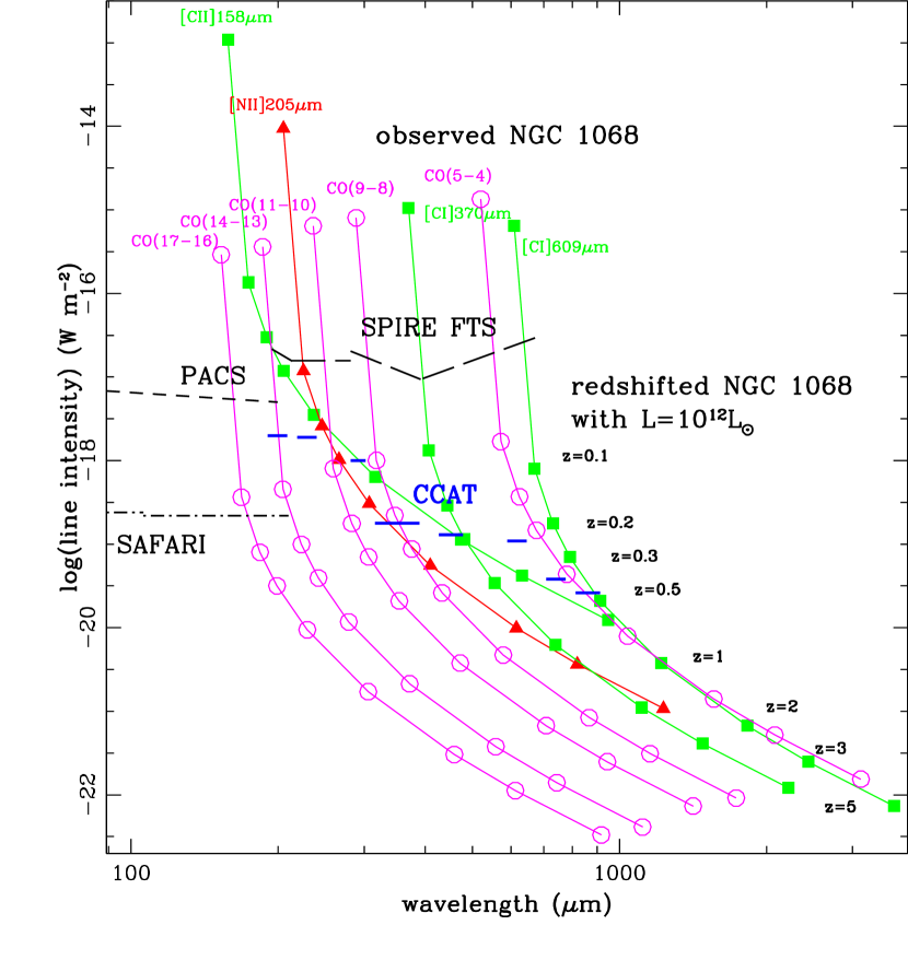
Figure 14.— Left panel: Comparison between the observed far-IR/submillimetre lines of NGC 1068 with the predictions of the same lines as a function of redshift of a similar galaxy with an intrinsic luminosity of L=10¹²L_☉. The stellar/HII region lines are shown as filled triangles (in red), the low-ionization/PDR lines are shown as filled squares (in green), while the molecular lines are shown as open circles (in magenta). For comparison, we overplot the 5$\sigma$ (in 1 hr) sensitivity threshold of Herschel-PACS, Herschel-SPIRE, SPICA-SAFARI and CCAT. See Spinoglio et al. (2012) for more details on the assumed sensitivities of the future SAFARI and CCAT instruments. Right panel: Same diagram for other two templates: the starburst galaxy M82 (Kamenetzky et al., 2012) and the ULIRG Arp220 (Rangwala et al., 2011).

4. Summary and conclusions

We summarize here the results of this work. The first complete submillimetre (190–670 $\mu$m) spectrum of the Seyfert type 2 galaxy NGC 1068 reveals the full sequence of CO pure rotational lines from J_up=4 to J_up=13. The radiation transfer analysis of these lines shows the presence of two physically distinct components: the first one originating from the circum-nuclear disk (CND) of few arcseconds in diameter ($\sim$ 4$\arcsec$) and the second one excited in the star forming ring (SF-ring) with a diameter ten times larger ($\sim$ 40$\arcsec$). These results indicate a kinetic temperature of CO of $T_{\rm kin}$=100 K and 127 K, a gas density of $n({\rm H_{2}})$=$10^{4.5}$ and $10^{2.9}$ cm^-3 and a derived molecular hydrogen mass of M(H₂) $\sim$ 2.4$\times$10⁷ M_☉ and M(H₂) $\sim$ 3.5$\times$10⁸ M_☉, for the compact and extended regions, respectively.

The comparison of the observed CO line intensities with predictions of photodissociation (PDR) and X-ray dominated regions (XDR) models shows that the circum-nuclear disk emission can be modeled equally well by both types of models, while the CO lines in the star-forming ring can be modeled by a photodissociation region only. However some observational constraints, such as the total CO surface brightness and the required radiation field, indicate that the most plausible explanation for the CO excitation of the CND is an XDR with density of n(H₂) $\sim$ 10⁴ cm^-3 and X-ray flux of 9 erg s^-1 cm^-2, consistent with the AGN illumination. In contrast, the excitation of the SF-ring component is due to PDR emission originating from the young stars/HII regions in the spiral arms.

The water lines that we have detected with SPIRE, together with those observed by PACS (S. Hailey-Dunsheath 2012, private comm.), have been modeled with an LVG model to constrain the physical conditions of the water excitation. We have found that the kinetic temperature is T_kin=40 K, the molecular hydrogen density is $n(H_{2})=4\times 10^{6}-8\times 10^{7}$ and the column density is of order N(H₂O)=8 $\times 10^{17}$ cm^-2 for both water forms.

The computed column densities of the molecular ions detected (H₂O⁺ and OH⁺ ) are in agreement with PDR models that include cosmic ray ionization.

The fundamental rotational transition of HF has been detected in emission in NGC 1068 and we infer a column density of N(HF)$\sim 7.5\times 10^{12}$ cm^-2.

For the two [CI] transitions, we derived a kinetic temperature of 22.5$\pm$2.4 K in LTE approximation, which is much lower than the temperatures traced from the intermediate-J CO molecular gas.

The molecular masses that we derived from our analysis are in good agreement with the masses estimated from both CO interferometric measurements of low-J lines and mid-infrared H₂ emission lines.

Finally we show that the intermediate-J CO and [CI] lines in galaxies with L$\sim 10^{12}L_{\sun}$ can be observed from planned and future ground-based and space telescopes up to redshift of z $\sim$ 0.5, making their diagnostic power an important tool to study galaxy evolution at intermediate redshift.

Table 1 Fluxes of the molecular and atomic lines detected in the SPIRE FTS spectrum of NGC 1068 and compared to literature data

species	line id.	rest. freq.	$E_{\mathrm{up}}/\kappa_{B}$	Beam	Flux	1$\sigma$ Stat. Uncert.	1$\sigma$ Tot. Uncert.	Ref.
				FWHM
		(GHz)	(K)	($\arcsec$)	(10-17 W m-2)
compact source
12CO	J = 1-0	0115.271	5.53	1 $\times$ 0.8	.050	.001	0.01	1
	J = 2-1	0230.538	16.60	1 $\times$ 0.8	.360	.003	0.07	1
	J = 3-2	0345.796	33.19	1 $\times$ 0.8	2.36	0.34	0.50	1
	J = 9-8	1036.912	248.88	18.7	15.41	0.15	1.55	2
	J = 10-9	1151.985	304.16	17.1	14.32a	0.23	1.45	2
	J = 11-10	1267.014	364.97	17.6	12.80	0.15	1.29	2
	J = 12-11	1381.995	431.29	16.9	10.97	0.18	1.11	2
	J = 13-12	1496.923	503.13	16.8	6.11	0.27	0.67	2
o-H2O	$3_{12}-3_{03}$+	1097.365	215.1	18.7	4.15	0.03	0.42	2
	$3_{21}-3_{12}$+	1162.912	271.0	17.1	5.80	0.14	0.60	2
	$2_{21}-2_{12}$	1661.008	159.8	12.7	4.8	$\cdots$	1.6	3
	$2_{12}-1_{01}$	1669.905	80.1	12.7	14.3	$\cdots$	4.3	3
	$3_{03}-2_{12}$	1716.769	162.5	12.3	6.9	$\cdots$	2.2	3
	$4_{14}-3_{03}$	2640.474	289.2	8.0	5.1b	$\cdots$	1.6	3
	$2_{21}-1_{10}$	2773.978	159.8	7.6	6.5	$\cdots$	2.1	3
p-H2O	$2_{11}-2_{02}$+	0752.033	136.9	33.4	3.42	0.07	0.35	2
	$2_{02}-1_{11}$+	0987.927	100.8	19.8	6.09	0.11	0.62	2
	$1_{11}-0_{00}$+	1113.343	53.4	18.7	3.49	0.05	0.35	2
	$2_{20}-2_{11}$+	1228.789	195.9	17.6	5.30	0.09	0.54	2
	$3_{22}-3_{13}$	1919.359	296.8	9.8	2.4	$\cdots$	0.8	3
	$3_{13}-2_{02}$	2164.132	204.7	11.5	6.9	$\cdots$	2.2	3
o-H2O+	$1_{11}-0_{00}$ J=3/2-1/2	1115.204	53.5	18.7	2.13	0.05	0.22	2
o-H2O+	$1_{11}-0_{00}$ J=1/2-1/2	1139.561	53.5	17.1	1.98	0.09	0.22	2
OH+	1${}_{12}-0_{12}$	1033.118	49.6	18.7	4.34	0.16	0.46	2
CH+	J = 1-0	835.079	39.6	35.0	3.16	0.08	0.33	2
HF	J = 1-0	1232.476	59.1	17.6	2.16	0.09	0.23	2
[NII]	${}^{3}P_{1}-^{3}P_{0}$	1461.134	6.77	16.8	54.97	1.42	5.67	2
extended source
12CO	J = 2-1	230.538	16.60	31.0	6.41	.015	1.3	4
	J = 3-2	345.796	33.19	43.4	19.4	$\cdots$	3.4	5
	J = 4-3	461.041	55.32	43.4	21.69	0.66	2.73	6
	J = 5-4	576.268	82.97	43.4	26.80	0.43	3.30	6
	J = 6-5	691.473	116.16	43.4	24.73	0.24	3.02	6
	J = 7-6	806.652	154.87	43.4	21.06	1.30	2.88	6
	J = 8-7	921.800	199.11	43.4	19.78	0.64	2.50	6
[CI]	${}^{3}P_{1}-^{3}P_{0}$	492.161	23.62	43.4	12.81	0.13	1.57	6
	${}^{3}P_{2}-^{3}P_{1}$	809.342	62.46	43.4	21.08	1.20	2.84	6
[NII]	${}^{3}P_{1}-^{3}P_{0}$	1461.134	6.77	43.4	187.9	8.2	24.3	6

Note. — ^a This line is possibly contaminated by the o-H₂O $3_{12}-2_{21}$ at 1153.127 GHz. However, the line fitting results indicate that the CO line is dominant; therefore we assign the whole flux to the CO line; ^b This line is blended with the CO (23–22) transition, so to obtain the flux of water we subtracted the flux of CO (23–22) predicted by the model presented by Hailey-Dunsheath et al. (2012).

References. — (1): Interferometric observations from Krips et al. (2011), adding together the emission from the E-knot and the W-knot and using the conversion: $f({\rm W~{}m^{-2}})=3.33\times 10^{-23}\nu_{GHz}S_{CO}({\rm Jy~{}km~{}s^{-1}})$; (2): This work, SPIRE-FTS deep pointed spectrum; (3): S. Hailey-Dunsheath, 2012, private communication; (4): From CSO Z-Spec observations of Kamenetzky et al. (2011), using the same conversion as for (1); (5): C. Wilson, 2012, private communication; (6): This work, SPIRE-FTS line maps

Table 2RADEX Model Parameters and Ranges

Parameter	Range	# of Points
$T_{kin}$ [K]	$10^{1.7}-10^{3.5}$	90
$n(H_{2})$ [cm-3]	$10^{1.0}-10^{5.0}$	90
$N_{\rm CO}$ [cm-2]	$10^{16}-10^{20}$	90
$\Delta V$ [km s-1]	1.0	fixed

Note. — All parameters are sampled evenly in log space.

Table 3Multi-Component Radiative Transfer Results

Parameter	Median	1$\sigma$ Range	1D Max	4D Max
compact source
$T_{\rm kin}$ [K]	92	74 $-$ 120	87	100
$n({\rm H_{2}})$ [cm-3]	$10^{4.6}$	$10^{4.4}-10^{4.8}$	$10^{4.6}$	$10^{4.5}$
$N_{CO}$ [cm-2]	$10^{19.5}$	$10^{19.3}-10^{19.7}$	$10^{19.5}$	$10^{19.6}$
$\Phi_{\rm A}$	$10^{-0.9}$	$10^{-1.0}-10^{-0.9}$	$10^{-0.9}$	$10^{-0.9}$
$P$ [K cm-2]	$10^{6.6}$	$10^{6.5}-10^{6.8}$	$10^{6.6}$	$10^{6.6}$
$\langle N_{\rm CO}\rangle$ [cm-2]	$10^{18.6}$	$10^{18.4}-10^{18.7}$	$10^{18.6}$	$10^{18.6}$
M(H2) [M⊙]	$10^{7.4}$	$10^{7.2}-10^{7.5}$	$10^{7.4}$	$10^{7.4}$
extended source
$T_{\rm kin}$ [K]	116	80 $-$ 166	121	127
$n({\rm H_{2}})$ [cm-3]	$10^{2.8}$	$10^{2.3}-10^{3.3}$	$10^{2.9}$	$10^{2.9}$
$N_{CO}$ [cm-2]	$10^{18.8}$	$10^{18.3}-10^{19.3}$	$10^{18.7}$	$10^{18.7}$
$\Phi_{\rm A}$	$10^{-1.2}$	$10^{-1.3}-10^{-1.0}$	$10^{-1.2}$	$10^{-1.1}$
$P$ [K cm-2]	$10^{4.7}$	$10^{4.3}-10^{5.2}$	$10^{4.4}$	$10^{4.4}$
$\langle N_{\rm CO}\rangle$ [cm-2]	$10^{17.7}$	$10^{17.2}-10^{18.2}$	$10^{17.6}$	$10^{17.6}$
M(H2) [M⊙]	$10^{8.5}$	$10^{8.0}-10^{9.0}$	$10^{8.5}$	$10^{8.5}$

Note. — 1D max refers to the maximum value of the integrated parameter distribution. 4D max refers to the value of that parameter at the best fit solution.

Table 4The best fit model parameters of H₂O

Parameter	Value
Temperature	$40\pm 10$ K
density	$4\times 10^{6}-8\times 10^{7}$ cm-3
diameter	10${}^{\prime\prime}\pm 2^{\prime\prime}$
$N$(o-H2O)	$2\times 10^{17}-10^{18}$ cm-2
$N$(p-H2O)	$5\times 10^{16}-10^{18}$ cm-2

References

- Aalto et al. (2011) Aalto, S., Costagliola, F., van der Tak, F., & Meijerink, R. 2011, A&A, 527, A69
- Antonucci (1993) Antonucci, R. 1993, ARA&A, 31, 473
- Antonucci & Miller (1985) Antonucci, R. R. J., & Miller, J. S. 1985, ApJ, 297, 621
- Bendo et al. (2012) Bendo, G. J., et al. 2012, MNRAS, 419, 1833
- Bland-Hawthorn et al. (1997) Bland-Hawthorn, J., Gallimore, J. F., Tacconi, L. J., Brinks, E., Baum, S. A., Antonucci, R. R. J., & Cecil, G. N. 1997, Ap&SS, 248, 9
- Ceccarelli et al. (1998) Ceccarelli, C., et al. 1998, A&A, 331, 372
- Clegg et al. (1996) Clegg, P. E., et al. 1996, A&A, 315, L38
- Colbert et al. (2002) Colbert, E. J. M., Weaver, K. A., Krolik, J. H., Mulchaey, J. S., & Mushotzky, R. F. 2002, ApJ, 581, 182
- Daniel et al. (2011) Daniel, F., Dubernet, M.-L., & Grosjean, A. 2011, A&A, 536, A76
- Daniel et al. (2010) Daniel, F., Dubernet, M.-L., Pacaud, F., & Grosjean, A. 2010, A&A, 517, A13
- de Graauw et al. (1996) de Graauw, T., et al. 1996, A&A, 315, L49
- Draine (1978) Draine, B. T. 1978, ApJS, 36, 595
- Dubernet et al. (2009) Dubernet, M.-L., Daniel, F., Grosjean, A., & Lin, C. Y. 2009, A&A, 497, 911
- Dubernet et al. (2006) Dubernet, M.-L., Grosjean, A., Flower, D., Roueff, E., Daniel, F., Moreau, N., & Debray, B. 2006, Journal of Plasma Research SERIES, Volume 7, p. 356-357, 7, 356
- Fulton et al. (2010) Fulton, T. R., et al. 2010, in Society of Photo-Optical Instrumentation Engineers (SPIE) Conference Series, Vol. 7731, Society of Photo-Optical Instrumentation Engineers (SPIE) Conference Series
- Gallimore et al. (2004) Gallimore, J. F., Baum, S. A., & O’Dea, C. P. 2004, ApJ, 613, 794
- García-Burillo et al. (2010) García-Burillo, S., et al. 2010, A&A, 519, A2
- Goldsmith & Langer (1999) Goldsmith, P. F. and Langer, W. D.1999, ApJ, 517, 209
- González-Alfonso et al. (2010) González-Alfonso, E., et al. 2010, A&A, 518, L43
- Griffin et al. (2010) Griffin, M. J., et al. 2010, A&A, 518, L3
- Hailey-Dunsheath et al. (2012) Hailey-Dunsheath, S., et al. 2012, ArXiv e-prints
- Hollenbach et al. (2012) Hollenbach, D., Kaufman, M. J., Neufeld, D., Wolfire, M., & Goicoechea, J. R. 2012, eprint arXiv:1205.6446
- Jaffe et al. (2004) Jaffe, W., et al. 2004, Nature, 429, 47
- Kamenetzky et al. (2011) Kamenetzky, J., et al. 2011, ApJ, 731, 83
- Kamenetzky et al. (2012) —. 2012, ApJ, 753, 70
- Kaufman et al. (2006) Kaufman, M. J., Wolfire, M. G., & Hollenbach, D. J. 2006, ApJ, 644, 283
- Kessler et al. (1996) Kessler, M. F., et al. 1996, A&A, 315, L27
- Kohno et al. (2008) Kohno, K., Nakanishi, K., Tosaki, T., Muraoka, K., Miura, R., Ezawa, H., & Kawabe, R. 2008, Ap&SS, 313, 279
- Krips et al. (2006) Krips, M., Eckart, A., Neri, R., Schödel, R., Leon, S., Downes, D., García-Burillo, S., & Combes, F. 2006, A&A, 446, 113
- Krips et al. (2011) Krips, M., et al. 2011, ApJ, 736, 37
- Krips et al. (2008) Krips, M., Neri, R., García-Burillo, S., Martín, S., Combes, F., Graciá-Carpio, J., & Eckart, A. 2008, ApJ, 677, 262
- Lutz et al. (2000) Lutz, D., Sturm, E., Genzel, R., Moorwood, A. F. M., Alexander, T., Netzer, H., & Sternberg, A. 2000, ApJ, 536, 697
- Maloney et al. (1996) Maloney, P. R., Hollenbach, D. J., & Tielens, A. G. G. M. 1996, ApJ, 466, 561
- Meijerink & Spaans (2005) Meijerink, R., & Spaans, M. 2005, A&A, 436, 397
- Meijerink et al. (2007) Meijerink, R., Spaans, M., & Israel, F. P. 2007, A&A, 461, 793
- Monje et al. (2011) Monje, R. R., Phillips, T. G., Peng, R., Lis, D. C., Neufeld, D. A., & Emprechtinger, M. 2011, ApJ, 742, L21
- Müller et al. (2005) Müller, H. S. P., Schlöder, F., Stutzki, J., & Winnewisser, G. 2005, Journal of Molecular Structure, 742, 215
- Müller et al. (2001) Müller, H. S. P., Thorwirth, S., Roth, D. A., & Winnewisser, G. 2001, A&A, 370, L49
- Müller Sánchez et al. (2009) Müller Sánchez, F., Davies, R. I., Genzel, R., Tacconi, L. J., Eisenhauer, F., Hicks, E. K. S., Friedrich, S., & Sternberg, A. 2009, ApJ, 691, 749
- Naylor et al. (2010a) Naylor, B. J., et al. 2010a, ApJ, 722, 668
- Naylor et al. (2010b) Naylor, D. A., et al. 2010b, in Society of Photo-Optical Instrumentation Engineers (SPIE) Conference Series, Vol. 7731, Society of Photo-Optical Instrumentation Engineers (SPIE) Conference Series
- Neufeld & Wolfire (2009) Neufeld, D. A., & Wolfire, M. G. 2009, ApJ, 706, 1594
- Pickett et al. (1998) Pickett, H. M., Poynter, R. L., Cohen, E. A., Delitsky, M. L., Pearson, J. C., & Müller, H. S. P. 1998, J. Quant. Spec. Radiat. Transf., 60, 883
- Pier et al. (1994) Pier, E. A., Antonucci, R., Hurt, T., Kriss, G., & Krolik, J. 1994, ApJ, 428, 124
- Pilbratt et al. (2010) Pilbratt, G. L., et al. 2010, A&A, 518, L1
- Poglitsch et al. (2010) Poglitsch, A., et al. 2010, A&A, 518, L2
- Rangwala et al. (2011) Rangwala, N., et al. 2011, ApJ, 743, 94
- Rigopoulou et al. (2002) Rigopoulou, D., Kunze, D., Lutz, D., Genzel, R., & Moorwood, A. F. M. 2002, A&A, 389, 374
- Röllig et al. (2007) Röllig, M., et al. 2007, A&A, 467, 187
- Rotaciuc et al. (1991) Rotaciuc, V., Krabbe, A., Cameron, M., Drapatz, S., Genzel, R., Sternberg, A., & Storey, J. W. V. 1991, ApJ, 370, L23
- Schinnerer et al. (2000) Schinnerer, E., Eckart, A., Tacconi, L. J., Genzel, R., & Downes, D. 2000, ApJ, 533, 850
- Schöier et al. (2005) Schöier, F. L., van der Tak, F. F. S., van Dishoeck, E. F., & Black, J. H. 2005, A&A, 432, 369
- Scoville et al. (1988) Scoville, N. Z., Matthews, K., Carico, D. P., & Sanders, D. B. 1988, ApJ, 327, L61
- Spinoglio et al. (2012) Spinoglio, L., Dasyra, K. M., Franceschini, A., Gruppioni, C., Valiante, E., & Isaak, K. 2012, ApJ, 745, 171
- Spinoglio et al. (2005) Spinoglio, L., Malkan, M. A., Smith, H. A., González-Alfonso, E., & Fischer, J. 2005, ApJ, 623, 123
- Tacconi et al. (1994) Tacconi, L. J., Genzel, R., Blietz, M., Cameron, M., Harris, A. I., & Madden, S. 1994, ApJ, 426, L77
- Thatte et al. (1997) Thatte, N., Quirrenbach, A., Genzel, R., Maiolino, R., & Tecza, M. 1997, ApJ, 490, 238
- Thronson et al. (1989) Thronson, Jr., H. A., et al. 1989, ApJ, 343, 158
- Tsai et al. (2012) Tsai, M., Hwang, C.-Y., Matsushita, S., Baker, A. J., & Espada, D. 2012, ApJ, 746, 129
- Usero et al. (2004) Usero, A., García-Burillo, S., Fuente, A., Martín-Pintado, J., & Rodríguez-Fernández, N. J. 2004, A&A, 419, 897
- van der Tak et al. (2008) van der Tak, F. F. S., Aalto, S., & Meijerink, R. 2008, A&A, 477, L5
- van der Tak et al. (2007) van der Tak, F. F. S., Black, J. H., Schöier, F. L., Jansen, D. J., & van Dishoeck, E. F. 2007, A&A, 468, 627
- van der Werf et al. (2010) van der Werf, P. P., et al. 2010, A&A, 518, L42
- Ward et al. (2003) Ward, J. S., Zmuidzinas, J., Harris, A. I., & Isaak, K. G. 2003, ApJ, 587, 171
- Wolfire et al. (2010) Wolfire, M. G., Hollenbach, D., & McKee, C. F. 2010, ApJ, 716, 1191
- Yang et al. (2010) Yang, B., Stancil, P. C., Balakrishnan, N., & Forrey, R. C. 2010, ApJ, 718, 1062