Non-divisiblity and non-Markovianity in a Gaussian dissipative dynamics

Abstract

We study a stochastic Schrödinger equation that generates a family of Gaussian dynamical maps in one dimension permitting a detailed exam of two different definitions of non-Markovianity: one related to the explicit dependence of the generator on the starting time, the other to the non-divisibility of the time-evolution maps. The model shows instances where one has non-Markovianity in both senses and cases when one has Markovianity in the second sense but not in the first one.

Recent theoretical and experimental advances have aroused a lot of interest in non-Markovian effects when quantum systems interact with an environment which cannot be considered at equilibrium [1]-[15]. More specifically, consider a system $S$ embedded in an environment $E$, under the hypothesis of an initial factorized state, i.e., a density matrix of the form $\rho\otimes\rho_{E}$; tracing away the environment degrees of freedom obtains an exact completely positive (CP) reduced dynamics for $S$ that sends an initial state $\rho$ at time $t_{0}\geq 0$ into a state $\rho_{t,t_{0}}$ at time $t\geq t_{0}$. This irreversible time-evolution is generated by an integro-differential equation of the form

$$\partial_{t}\rho_{t,t_{0}}=\int_{t_{0}}^{t}{\rm d}u\,K_{t,u}[\rho_{u,t_{0}}]\ ,\quad\rho_{t_{0},t_{0}}=\rho\ ,$$ (1)

where the operator kernel embodies the dependence on the past history of the system. The previous equation can be cast in the convolution-less form [10]

$$\partial_{t}\rho_{t,t_{0}}=\mathbb{L}_{t,t_{0}}[\rho_{t,t_{0}}]\ ,$$ (2)

where the presence of memory effects is now incorporated in the dependence of the generator on the initial time $t_{0}$. Because of this, the CP maps which solve (2),

$$\Gamma_{t,t_{0}}=\mathcal{T}\exp\Bigg{(}\int_{t_{0}}^{t_{1}}{\rm d}u\,\mathbb{L}_{u,t_{0}}\Bigg{)}\ ,$$ (3)

with $\mathcal{T}$ time-ordering, violate, in general, the (two-parameter) semigroup composition law, namely

$$\Gamma_{t,t_{1}}\circ\Gamma_{t_{1},t_{0}}\neq\Gamma_{t,t_{0}}\ ,\qquad 0\leq t_{0}\leq t_{1}\leq t\ .$$ (4)

Indeed, if $\mathbb{L}_{u,t_{0}}=\mathbb{L}_{u}$ then (3) yields the equality in (4); vice versa, if in (4) the equality holds, by taking the time derivative of both sides with respect to $t$ one obtains $\mathbb{L}_{t,t_{1}}=\mathbb{L}_{t,t_{0}}$ for all $t_{1}\geq t_{0}\geq 0$. In [10], the dependence of the generator $\mathbb{L}_{t,t_{0}}$ on $t_{0}$ and thus (4) is taken as a criterion of non-Markovianity.

On the other hand, in [12]– [14] a different approach is considered whereby, given a one-parameter family of CP maps $\gamma_{t}$, $t\geq 0$, their non-Markovianity is related to non-divisibility, namely to the fact that no CP map $\Lambda_{t,u}$, $t\geq u\geq 0$, exists that connects the maps $\gamma_{t}$. In other words, the criterion of non-Markovianity becomes

$$\gamma_{t}=\Lambda_{t,u}\circ\gamma_{u}\Longrightarrow\Lambda_{t,t_{0}}\quad\hbox{not CP}\ .$$ (5)

If a CP $\Lambda_{t,u}$ existed, it would follow that certain CP monotone like the trace distance, the fidelity or the relative entropy should be decreasing: then, non-Markovianity is identified by the increase in time of such quantities which can also be taken as a measure of non-Markovianity.

In order to study the two criteria of non-Markovianity, we consider a stochastic Schrödinger equation originally proposed as a non-Markovian mechanism for the wave function collapse [16]. Specifically, we take a particle in one dimension subjected to a time-dependent random Hamiltonian of the form (for sake of simplicity, in the following, vector and matrix multiplication will be understood)

$$\hat{H}^{\boldsymbol{w}}_{t}=\hat{H}-\,{\boldsymbol{w}}^{T}(t)\,\hat{{\boldsymbol{r}}}\ ,$$ (6)

where the Hamiltonian $\hat{H}$ is at most quadratic in position and momentum operators $\hat{{\boldsymbol{r}}}^{T}=(\hat{r}_{1},\hat{r}_{2})=(\hat{q},\hat{p})$, while ${\boldsymbol{w}}^{T}(t)=(w_{1}(t),w_{2}(t))$ is a Gaussian noise vector with zero mean and $2\times 2$ correlation matrix ${\boldsymbol{D}}(t,s)$:

$$\Big{[}{\boldsymbol{D}}(t,s)\Big{]}_{ij}={\langle\!\langle}w_{i}(t)\,w_{j}(s){\rangle\!\rangle},$$ (7)

where ${\langle\!\langle}\cdot{\rangle\!\rangle}$ denotes the average over the noise. This latter matrix is real symmetric, $D_{ij}(t,s)=D_{ji}(s,t)$, and of positive-definite type, that is

$$\sum_{i,j;t_{a},t_{b}}\xi_{i}(t_{a})\xi_{j}(t_{b})\,D_{ij}(t_{a},t_{b})\geq 0\ ,\ \forall\ \xi(t_{a})\in\mathbbm{R}^{2}\ ,$$ (8)

for any choice of times $\{t_{a}\}_{a=1}^{n}$. For each realization of the noise, the Schrödinger equation ($\hbar=1$)

$$i\frac{{\rm d}|\psi^{\boldsymbol{w}}_{t}\rangle}{{\rm d}t}=\left[\hat{H}-{\boldsymbol{w}}^{T}(t)\,\hat{{\boldsymbol{r}}}\right]|\psi_{t}^{\boldsymbol{w}}\rangle\ ,$$ (9)

generates unitary maps $\hat{U}^{\boldsymbol{w}}_{t,t_{0}}$ on the system Hilbert space that send an initial vector state $|\psi\rangle$ at time $t=t_{0}$ into $|\psi^{\boldsymbol{w}}_{t,t_{0}}\rangle$ at time $t$. Averaging the projector $|\psi^{\boldsymbol{w}}_{t,t_{0}}\rangle\langle\psi^{\boldsymbol{w}}_{t,t_{0}}|$ over the noise yields a density matrix

$$\rho_{t,t_{0}}={\langle\!\langle}\,|\psi^{\boldsymbol{w}}_{t,t_{0}}\rangle\langle\psi_{t,t_{0}}^{\boldsymbol{w}}|{\rangle\!\rangle}\ .$$ (10)

In order to find $\hat{U}^{\boldsymbol{w}}_{t,t_{0}}$, one first goes to the interaction representation and sets:

$$|\widetilde{\psi}^{\boldsymbol{w}}_{t,t_{0}}\rangle = \hat{U}^{\dagger}_{t-t_{0}}|\psi^{\boldsymbol{w}}_{t,t_{0}}\rangle\ ,$$

$$i\frac{{\rm d}|\widetilde{\psi}_{t,t_{0}}^{\boldsymbol{w}}\rangle}{{\rm d}t} = {\boldsymbol{w}}^{T}(t)\,\hat{{\boldsymbol{r}}}(t-t_{0})\,|\widetilde{\psi}_{t,t_{0}}^{\boldsymbol{w}}\rangle\ ,$$ (11)

where $\hat{U}_{t}=\exp(-i\,\hat{H}\,t)$ and:

$$\hat{{\boldsymbol{r}}}(t)=\hat{U}_{t}^{\dagger}\,\hat{{\boldsymbol{r}}}\,\hat{U}_{t}\equiv{\boldsymbol{S}}_{t}\hat{{\boldsymbol{r}}}\ ,$$ (12)

${\boldsymbol{S}}_{t}$ being a suitable symplectic matrix. For a given realization of the noise ${\boldsymbol{w}}(t)$, the solution is of the form $|\widetilde{\psi}^{\boldsymbol{w}}_{t,t_{0}}\rangle=\widetilde{U}^{\boldsymbol{w}}_{t,t_{0}}|\psi\rangle$ where, a part for a pure phase,

$$\widetilde{U}^{\boldsymbol{w}}_{t,t_{0}}=\exp\left\{-i\int_{t_{0}}^{t}{\rm d}u\,\hat{{\boldsymbol{w}}}^{T}(u)\,\hat{{\boldsymbol{r}}}(u-t_{0})\right\}$$ (13)

$$|\psi^{\boldsymbol{w}}_{t,t_{0}}\rangle=\hat{U}_{t-t_{0}}\hat{U}^{\boldsymbol{w}}_{t,t_{0}}\,|\psi\rangle\ .$$ (14)

By averaging over the noise, the corresponding density matrix (10) satisfies:

$$i\partial_{t}\rho_{t,t_{0}}=\Big{[}\hat{H},\rho_{t,t_{0}}\Big{]}-\sum_{j=1}^{2}\Big{[}\hat{r}_{j},{\langle\!\langle}w_{j}(t)|\psi^{\boldsymbol{w}}_{t,t_{0}}\rangle\langle\psi_{t,,t_{0}}^{\boldsymbol{w}}|{\rangle\!\rangle}\Big{]}\ .$$

This stochastic Liouville equation can be turned into a standard master equation by means of the Furutsu-Novikov-Donsker relation [17]:

$${\langle\!\langle}{\boldsymbol{w}}(s)\boldsymbol{X}[{\boldsymbol{w}}]{\rangle\!\rangle}=\int_{-\infty}^{+\infty}\hskip-14.22636pt{\rm d}u\,{\langle\!\langle}{\boldsymbol{w}}(s){\boldsymbol{w}}(u){\rangle\!\rangle}\,{\langle\!\langle}\frac{\delta R[{\boldsymbol{w}}]}{\delta{\boldsymbol{w}}(u)}{\rangle\!\rangle}\ ,$$ (15)

where $\boldsymbol{X}[{\boldsymbol{w}}]$ is a functional of the noise, $\delta/{\delta{\boldsymbol{w}}(u)}$ denotes the functional derivative with respect to the noise and $R[{\boldsymbol{w}}]$ is the density operator of the system. With $R[{\boldsymbol{w}}]=|\psi^{\boldsymbol{w}}_{t,t_{0}}\rangle\langle\psi_{t,t_{0}}^{\boldsymbol{w}}|$, one gets:

$$\partial_{t}\rho_{t,t_{0}}=\mathbb{L}_{t,t_{0}}[\rho_{t,t_{0}}]=-i\Big{[}\hat{H},\rho_{t,t_{0}}\Big{]}+\mathbb{N}_{t,t_{0}}[\rho_{t,t_{0}}]$$ (16)

with:

$$\mathbb{N}_{t,t_{0}}[\rho] =\sum_{i,j=1}^{2}C_{ij}(t,t_{0})\,\Big{(}\hat{r}_{i}\,\rho\,\hat{r}_{j}-\frac{1}{2}\Big{\{}\hat{r}_{j}\hat{r}_{i},\rho\Big{\}}\Big{)}$$ (17)

$$\boldsymbol{C}(t,t_{0}) =\int_{t_{0}}^{t}{\rm d}u\,\Big{[}{\boldsymbol{D}}(t,u)\,{\boldsymbol{S}}_{u-t}+{\boldsymbol{S}}^{T}_{u-t}{\boldsymbol{D}}^{T}(t,u)\Big{]}\ .$$ (18)

If ${\boldsymbol{D}}(t,u)=\delta(t-u)\,{\boldsymbol{D}}$ (i.e., white noise) then one reduces to the Markovian Lindblad type dynamics with a time-independent positive Kossakowski matrix, namely $\boldsymbol{C}(t,t_{0})={\boldsymbol{D}}$ [18, 19]. In the time-dependent case, in order that the maps $\Gamma_{t,t_{0}}$ generated by $\mathbb{L}_{t,t_{0}}$ be CP, the Kossakowski matrix $\boldsymbol{C}(t,t_{0})$ need not to be positive, as we explicitly show in the following. We shall seek a solution of (16) in the form

$$\rho_{t,t_{0}}=\Gamma_{t,t_{0}}[\rho]=\int\frac{{\rm d}^{2}{\boldsymbol{r}}}{2\pi}\,G_{t,t_{0}}({\boldsymbol{r}})\,R({\boldsymbol{r}})\,\hat{W}({\boldsymbol{S}}_{t-t_{0}}{\boldsymbol{r}})\,,$$ (19)

where we have introduced the Weyl operators:

$$\hat{W}({\boldsymbol{r}})={\rm e}^{i\,{\boldsymbol{r}}^{T}{\boldsymbol{\Omega}}\,\hat{{\boldsymbol{r}}}}={\rm e}^{i(q\hat{p}-p\hat{q})}\ ,$$ (20)

with ${\boldsymbol{r}}^{T}=(q,p)\in{\mathbbm{R}}^{2}$ and $\displaystyle{\boldsymbol{\Omega}}=\begin{pmatrix}0&1\cr-1&0\end{pmatrix}$, and $R({\boldsymbol{r}})=\rm Tr[\rho\,\hat{W}(-{\boldsymbol{r}})]$ is related to the initial condition by:

$$\rho_{t_{0},t_{0}}=\rho=\int\frac{{\rm d}^{2}{\boldsymbol{r}}}{2\pi}\,R({\boldsymbol{r}})\,\hat{W}({\boldsymbol{r}})\,.$$

Because the Hamiltonian $\hat{H}$ is at most quadratic and the matrix $S_{t}$ in (12) is symplectic, one finds:

$$\hat{U}_{t}\,\hat{W}({\boldsymbol{r}})\,\hat{U}_{t}^{\dagger}=\hat{W}({\boldsymbol{S}}_{t}{\boldsymbol{r}})\ .$$

Direct insertion of (19) into (16) yields

$$\partial_{t}G_{t,t_{0}}({\boldsymbol{r}})=-\Big{[}{\boldsymbol{r}}^{T}\,{\boldsymbol{S}}^{T}_{t-t_{0}}\boldsymbol{C}(t,t_{0}){\boldsymbol{S}}_{t-t_{0}}\,{\boldsymbol{r}}\Big{]}\,G_{t,t_{0}}({\boldsymbol{r}})\,,$$

whence $G_{t,t_{0}}({\boldsymbol{r}})=\exp\left[-\frac{1}{2}\,{\boldsymbol{r}}^{T}\,{\boldsymbol{g}}(t,t_{0})\,{\boldsymbol{r}}\right]$ with

$${\boldsymbol{g}}(t,t_{0}) = 2\,\int_{t_{0}}^{t}{\rm d}u\,{\boldsymbol{S}}^{T}_{u-t_{0}}\boldsymbol{C}(u,t_{0}){\boldsymbol{S}}_{u-t_{0}}$$ (21)

$$= \int_{t_{0}}^{t}{\rm d}u\int_{t_{0}}^{t}\,{\rm d}v\,{\boldsymbol{S}}^{T}_{u-t_{0}}{\boldsymbol{D}}(u,v){\boldsymbol{S}}_{v-t_{0}}\ .$$ (22)

Furthermore, since ${\boldsymbol{D}}(u,v)$ is of positive type, the matrix ${\boldsymbol{g}}(t,t_{0})$ is positive definite and $G_{t,t_{0}}({\boldsymbol{r}})$ a real Gaussian function; the solution $\Gamma_{t,t_{0}}[\rho]$ can then be cast in a continuous Kraus-Stinespring decomposition which guarantees the complete positivity of the maps $\Gamma_{t,t_{0}}$. Let $G_{t,t_{0}}({\boldsymbol{r}})=\int_{\mathbb{R}^{2}}{\rm d}^{2}{\boldsymbol{x}}\,\delta({\boldsymbol{x}}-{\boldsymbol{r}})\,G_{t,t_{0}}({\boldsymbol{x}})$ with

$$\delta({\boldsymbol{x}}-{\boldsymbol{r}})=\frac{1}{(2\pi)^{2}}\int_{\mathbb{R}^{2}}{\rm d}^{2}{\boldsymbol{y}}\,{\rm e}^{i{\boldsymbol{y}}^{T}{\boldsymbol{\Omega}}({\boldsymbol{x}}-{\boldsymbol{r}})}\ .$$

By inserting it into (19) and using $\hat{W}({\boldsymbol{x}})\hat{W}({\boldsymbol{r}})\hat{W}^{\dagger}({\boldsymbol{x}})={\rm e}^{-i{\boldsymbol{x}}^{T}{\boldsymbol{\Omega}}{\boldsymbol{r}}}\hat{W}({\boldsymbol{r}})$, one rewrites

$$\Gamma_{t,t_{0}}[\rho]=\int_{\mathbb{R}^{2}}\frac{{\rm d}^{2}{\boldsymbol{y}}}{2\pi}F_{t,t_{0}}({\boldsymbol{y}})\,\hat{U}_{t-t_{0}}\hat{W}({\boldsymbol{x}})\,\rho\,\hat{W}^{\dagger}({\boldsymbol{x}})\hat{U}^{\dagger}_{t-t_{0}}\\$$ (23)

with the Fourier transform

$$F_{t,t_{0}}({\boldsymbol{y}})=\int_{\mathbb{R}^{2}}\frac{{\rm d}^{2}{\boldsymbol{x}}}{2\pi}\,{\rm e}^{i{\boldsymbol{y}}^{T}{\boldsymbol{\Omega}}{\boldsymbol{x}}}G_{t,t_{0}}({\boldsymbol{x}})\ ,$$ (24)

also a real Gaussian, hence a positive function.

Using (19) one can study the composition properties of the maps $\Gamma_{t,t_{0}}$; since:

$$\Gamma_{t_{2},t_{1}}\circ\Gamma_{t_{1},t_{0}}[\rho]=\int\frac{{\rm d}^{2}{\boldsymbol{r}}}{2\pi}\,G_{t_{2},t_{1}}({\boldsymbol{S}}_{t_{1}-t_{0}}{\boldsymbol{r}})\,G_{t_{1},t_{0}}({\boldsymbol{r}})\,R({\boldsymbol{r}})\,\hat{W}({\boldsymbol{S}}_{t_{2}-t_{0}}{\boldsymbol{r}}),$$

in order to to satisfy the semigroup composition law $\Gamma_{t_{2},t_{1}}\circ\Gamma_{t_{1},t_{0}}=\Gamma_{t_{1},t_{0}}$ one should have

$$G_{t_{2},t_{1}}({\boldsymbol{S}}_{t_{1}-t_{0}}{\boldsymbol{r}})\,G_{t_{1},t_{0}}({\boldsymbol{r}})=G_{t_{2},t_{0}}({\boldsymbol{r}})\,.$$

Using (22), one instead finds that

$$\Bigg{(}\int_{t_{1}}^{t_{2}}\int_{t_{1}}^{t_{2}}+\int_{t_{0}}^{t_{1}}\int_{t_{0}}^{t_{1}}{\rm d}u\,{\rm d}v\Bigg{)}\Bigg{(}{\boldsymbol{S}}^{T}_{u-t_{0}}{\boldsymbol{D}}(u,v){\boldsymbol{S}}_{v-t_{0}}\Bigg{)}$$

$$\hskip 142.26378pt\neq\int_{t_{0}}^{t_{2}}{\rm d}u\int_{t_{0}}^{t_{2}}{\rm d}v\,{\boldsymbol{S}}^{T}_{u-t_{0}}{\boldsymbol{D}}(u,v){\boldsymbol{S}}_{v-t_{0}}\ .$$ (25)

This fact remains true even when ${\boldsymbol{D}}(s,u)={\boldsymbol{D}}(|s-u|)$ in which case from (22) we have

$${\boldsymbol{g}}(t,t_{0})=\int_{0}^{t-t_{0}}{\rm d}u\int_{0}^{t-t_{0}}\,{\rm d}v\,{\boldsymbol{S}}^{T}_{u}{\boldsymbol{D}}(u,v){\boldsymbol{S}}_{v}$$

and $\Gamma_{t,t_{0}}=\Gamma_{t-t_{0},0}$.

Consider the master equation (16); if $t_{0}=0$ its solutions $\rho_{t,0}=\Gamma_{t,0}[\rho]$ propagate the initial state $\rho$ from $t_{0}=0$ to $t\geq 0$. Because of the above result, $\Gamma_{t,0}\neq\Gamma_{t,t_{0}}\circ\Gamma_{t_{0},0}$. However, setting $t_{0}=0$ in (16) and searching a solution $\Lambda_{t,t_{0}}[\rho]$ in the form (19), one gets

$$\Lambda_{t,t_{0}}[\rho]=\int\frac{{\rm d}^{2}{\boldsymbol{r}}}{2\pi}\,L_{t,t_{0}}({\boldsymbol{r}})\,R({\boldsymbol{r}})\,\hat{W}({\boldsymbol{S}}_{t-t_{0}}{\boldsymbol{r}})\\$$ (26)

where $L_{t,t_{0}}({\boldsymbol{r}})=\exp\left\{-\frac{1}{2}{\boldsymbol{r}}^{T}{\boldsymbol{\ell}}(t,t_{0}){\boldsymbol{r}}\right\}$ with:

$${\boldsymbol{\ell}}(t,t_{0}) = \int_{t_{0}}^{t}{\rm d}u\,{\boldsymbol{S}}^{T}_{u-t_{0}}\,\boldsymbol{C}(u,0)\,{\boldsymbol{S}}_{u-t_{0}}$$ (27)

$$= \int_{t_{0}}^{t}{\rm d}u\int_{0}^{u}{\rm d}v\,{\boldsymbol{S}}^{T}_{u-t_{0}}\,{\boldsymbol{D}}(u,v)\,{\boldsymbol{S}}_{v-t_{0}}\,.$$ (28)

The function $L_{t,t_{0}}(r)$ plays the role of $G_{t,t_{0}}({\boldsymbol{r}})$ in (19) to which it reduces when $t_{0}=0$; that is $\Lambda_{t,0}=\Gamma_{t,0}$. Note however that, in contrast to ${\boldsymbol{g}}(t,t_{0})$ in (21), in ${\boldsymbol{\ell}}(t,t_{0})$ one integrates $\boldsymbol{C}(u,0)$, not $\boldsymbol{C}(u,t_{0})$, from $t_{0}$ to $t$. As a consequence, $\Gamma_{t,0}=\Lambda_{t,t_{0}}\circ\Gamma_{t_{0},0}$; indeed,

$$\Lambda_{t,t_{0}}\circ\Gamma_{t_{0},0}[\rho]=\int_{\mathbb{R}^{2}}\frac{{\rm d}^{2}{\boldsymbol{r}}}{2\pi}\,L_{t,t_{0}}({\boldsymbol{S}}_{t_{0}}{\boldsymbol{r}})\,L_{t_{0},0}({\boldsymbol{r}})\,R({\boldsymbol{r}})\,\hat{W}({\boldsymbol{S}}_{t}{\boldsymbol{r}})\ ,$$

where now, unlike in (25),

$${\boldsymbol{S}}^{T}_{t_{0}}\,\ell(t,t_{0})\,{\boldsymbol{S}}_{t_{0}}+{\boldsymbol{\ell}}(t_{0},0) =\Bigg{(}\int_{t_{0}}^{t}\int_{0}^{u}+\int_{0}^{t_{0}}\int_{0}^{u}\Bigg{)}{\rm d}u\,{\rm d}v\,{\boldsymbol{S}}^{T}_{u}\,{\boldsymbol{D}}(u,v)\,{\boldsymbol{S}}_{v}$$

$$=\int_{0}^{t}{\rm d}u\int_{0}^{u}{\rm d}v\,{\boldsymbol{S}}^{T}_{u}\,{\boldsymbol{D}}(u,v)\,{\boldsymbol{S}}_{v}={\boldsymbol{\ell}}(t,0)\ .$$

However, contrary to the maps $\Lambda_{t,0}=\Gamma_{t,0}$ which, as we have seen, are CP, the maps $\Lambda_{t,t_{0}}$ cannot be CP as this would imply [9] the positive definiteness of the matrix $\boldsymbol{C}(t,t_{0})$ in (17). In fact, the maps $\Lambda_{t,t_{0}}$ are in general not even positive.

All these various possibilities can be seen in a concrete example; consider a free particle of unit mass, $\hat{H}=\hat{p}^{2}/2$, so that ${\boldsymbol{S}}_{t}=\begin{pmatrix}1&t\cr 0&1\end{pmatrix}$, and a diagonal noise with correlation matrix given by

$${\boldsymbol{D}}(t,u)=\frac{\gamma\,{\rm e}^{-\gamma|t-u|}}{2}\begin{pmatrix}d_{q}&0\cr 0&d_{p}\end{pmatrix}\ .$$ (29)

First suppose the noise couples only to the position operator: $d_{q}=1$, $d_{p}=0$; then, from (18),

$$\boldsymbol{C}(t,t_{0})=\begin{pmatrix}1-{\rm e}^{-\gamma(t-t_{0})}&\frac{{\rm e}^{-\gamma(t-t_{0})}[1+\gamma(t-t_{0})]-1}{2\gamma}\cr\frac{{\rm e}^{-\gamma(t-t_{0})}[1+\gamma(t-t_{0})]-1}{2\gamma}&0\end{pmatrix}$$ (30)

has a negative eigenvalue for all $t>t_{0}\geq 0$. In spite of the non-positivity of the Kossakowski matrix in (18), the maps $\Gamma_{t,t_{0}}$ in (23) are nevertheless CP for all $0\leq t_{0}\leq t$.

We consider, as initial condition at $t_{0}$, a Gaussian state $\rho_{\boldsymbol{\sigma}}$ with covariance matrix (CM) $\boldsymbol{\sigma}$ and zero first moments, ${\rm Tr}\left[\rho_{\boldsymbol{\sigma}}\,\hat{W}(-{\boldsymbol{r}})\right]=\exp\left\{-\frac{1}{2}{\boldsymbol{r}}^{T}\,({\boldsymbol{\Omega}}\,\boldsymbol{\sigma}\,{\boldsymbol{\Omega}}^{T})\,{\boldsymbol{r}}\right\}$. Using (19), $\Gamma_{t,t_{0}}$ maps $\rho_{\boldsymbol{\sigma}}$ to the Gaussian state ${\rm Tr}\left[\Gamma_{t,t_{0}}[\rho_{\boldsymbol{\sigma}}]\hat{W}({\boldsymbol{r}})\right]=\exp\left\{-\frac{1}{2}{\boldsymbol{r}}^{T}{\boldsymbol{\Omega}}^{T}\boldsymbol{\sigma}_{t,t_{0}}{\boldsymbol{\Omega}}{\boldsymbol{r}}\right\}$, where $\boldsymbol{\sigma}_{t,t_{0}}={\boldsymbol{S}}_{t-t_{0}}\boldsymbol{\sigma}{\boldsymbol{S}}^{T}_{t-t_{0}}+\widetilde{{\boldsymbol{g}}}(t,t_{0})$ with

$$\widetilde{{\boldsymbol{g}}}(t,t_{0})=\int_{t_{0}}^{t}{\rm d}u\,{\boldsymbol{\Omega}}^{T}\,{\boldsymbol{S}}^{T}_{u-t}\,\boldsymbol{C}(u,t_{0})\,{\boldsymbol{S}}_{u-t}\,{\boldsymbol{\Omega}}\ .$$ (31)

Instead, if the same initial condition is taken for the maps $\Lambda_{t,t_{0}}$, the matrix $\widetilde{{\boldsymbol{g}}}(t,t_{0})$ is to be substituted by

$$\widetilde{{\boldsymbol{\ell}}}(t,t_{0})=\int_{t_{0}}^{t}{\rm d}u\,{\boldsymbol{\Omega}}^{T}\,{\boldsymbol{S}}^{T}_{u-t}\,\boldsymbol{C}(u,0)\,{\boldsymbol{S}}_{u-t}\,{\boldsymbol{\Omega}}\ .$$ (32)

If we choose $\boldsymbol{\sigma}={\boldsymbol{S}}_{t_{0}-t}\boldsymbol{\sigma}_{0}{\boldsymbol{S}}^{T}_{t_{0}-t}$ and expand $\boldsymbol{\sigma}_{t,t_{0}}=\boldsymbol{\sigma}_{0}+\widetilde{{\boldsymbol{\ell}}}(t,t_{0})$ to first order about $t_{0}$, we have:

$$\boldsymbol{\sigma}_{t,t_{0}} \simeq\boldsymbol{\sigma}_{0}+(t-t_{0}){\boldsymbol{\Omega}}^{T}\,\boldsymbol{C}(t_{0},0)\,{\boldsymbol{\Omega}}\,,$$ (33)

where $\boldsymbol{C}(t_{0},0)$ is calculated from Eq. (30). Now, the second matrix at the l.h.s. is real symmetric and has one positive and one negative eigenvlaue, $\lambda\geq 0$ and $-\mu<0$; let ${\boldsymbol{V}}$ be the symplectic, orthogonal matrix which diagonalizes it. Then, choosing an initial state with CM diagonal in the same basis, i.e., $\boldsymbol{\sigma}_{0}={\rm Diag}[\sigma_{qq},\sigma_{pp}]$, such that $\boldsymbol{\sigma}_{0}+\frac{i}{2}{\boldsymbol{\Omega}}\geq 0$ (positivity of the initial state), one gets:

$$\boldsymbol{\sigma}_{t,t_{0}}\simeq{\boldsymbol{V}}^{T}\,\begin{pmatrix}\sigma_{qq}+\lambda(t-t_{0})&0\cr 0&\sigma_{pp}-\mu(t-t_{0})\end{pmatrix}\,{\boldsymbol{V}}\ ,$$

and a sufficiently small $\sigma_{pp}$ would yield a non positive-definite CM $\sigma_{t,t_{0}}$, thus exhibiting the non-positivity of the map $\Lambda_{t,t_{0}}$. The non-positive preserving character of $\Lambda_{t,t_{0}}$ is exposed by very specific states; on other states as, for instance, on all those of the form $\Gamma_{t_{0},0}[\rho]$ it acts perfectly well for $\Lambda_{t,t_{0}}\circ\Gamma_{t_{0},0}=\Gamma_{t,0}$. In addition, starting from $t_{0}=0$, $\Lambda_{t,0}=\Gamma_{t,0}$ is CP.

Therefore, in this case the master equation (16) generates a non-Markovian dynamics both according to the criterion (4), since the generator $\mathbb{L}_{t,t_{0}}$ depends on the initial time $t_{0}$ and also according to the other criterion (5). In fact, the family of maps $\Gamma_{t,0}$ is non-divisible for $\Lambda_{t,t_{0}}$ is uniquely defined and non-positive.

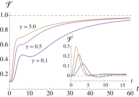
Figure 1: Plot of the time evolution of the fidelity ${\cal F}$ between two Gaussian states $\rho_{k}$, $k=1,2$, with zero first moments and CMs $\boldsymbol{\sigma}_{k}=\frac{1}{2}{\rm Diag}\left[\exp(2r_{k}),\exp(-2r_{k})\right]$, with $r_{1}=-r_{2}=1.5$, evolving under the map $\Gamma_{t,0}$ for different values of $\gamma$. The inset refers to the time derivative of the fidelity. The non-monotonic behavior denotes non-Markovian evolution [15]; note that as $\gamma$ increases, ${\cal F}$ becomes monotonic.

Since $\Lambda_{t,t_{0}}$ is not (completely) positive, certain quantities that exhibit monotonic behavior under CP maps fail to do so when evolving the system from time $t_{0}$ to time $t$. One of such quantities is the fidelity [15] $\mathcal{F}(t)=\mathcal{F}(\Gamma_{t,0}[\rho_{1}],\Gamma_{t,0}[\rho_{2}])$ of two states $\rho_{1}$ and $\rho_{2}$ evolving in time according to $\Gamma_{t,0}$. While $\mathcal{F}(t)\geq\mathcal{F}(0)$ for all $t\geq 0$, $\mathcal{F}(t_{0}+t)$ may become smaller than $\mathcal{F}(t_{0})$ for some $t,t_{0}>0$. This is showed in Fig. 1 for two Gaussian states with zero first moments and “squeezed” CM. As one may expect, the effect disappears when $\gamma$ increases towards the Markovian limit.

On the other hand, if in (9), the noise affects the particle momentum only, namely if $d_{q}=0$, $d_{p}=1$, then, from (29),

$$C(t,t_{0})=(1-{\rm e}^{-\gamma(t-t_{0})})\,\begin{pmatrix}0&0\cr 0&1\end{pmatrix}$$ (34)

is positive definite. It follows that the intertwining map $\Lambda_{t,t_{0}}$ is CP, whence the family of maps $\Gamma_{t,0}$ is divisible and Markovian according to the criterion (5). However, it is non-Markovian according to the other criterion (4). Indeed, the generator resulting from (9) depends on the starting time $t_{0}$.

In conclusion, the analysis of above examples indicates that the criterion identifying non-Markovianity with the explicit dependence of the generator ${\mathbb{L}}_{t,t_{0}}$ on the starting time $t_{0}$ appears stronger than the criterion based on the non-divisibility of the maps $\Gamma_{t,0}$. Indeed, on one hand, we have provided a case where the map $\Gamma_{t,0}$ is divisible, yet the generator of $\Gamma_{t,t_{0}}$ explicitly depends on the initial time $t_{0}$; on the other hand, a Markovian evolution according to the first criterion readily implies the semigroup composition law, i.e., (4) with the equality sign, hence divisibility of $\Gamma_{t,0}$. Nevertheless, the non-divisibility criterion is the only one at disposal when one is presented just with the family of maps $\Gamma_{t,0}$: in such a case, one may reconstruct the generator ${\mathbb{L}}_{t,0}$ starting from $t_{0}=0$, but, in general, no information is available on the full generator ${\mathbb{L}}_{t,t_{0}}$ at $t_{0}>0$.

Acknowledgments FB and RF thank A. Bassi and L. Ferialdi for useful discussions. SO acknowledges useful discussions with M. G. A. Paris and R. Vasile and financial support from MIUR (FIRB “LiCHIS” - RBFR10YQ3H) and from the University of Trieste (“FRA 2009”).

References

• [1] J. Wilkie, Phys. Rev. E 62, 8808 (2000).
• [2] A. A. Budini, Phys. Rev. A 69, 042107 (2004).
• [3] S. Maniscalco, Phys. Rev. A 72, 024103 (2005).
• [4] S. Maniscalco and F. Petruccione, Phys. Rev. A 73, 012111 (2006).
• [5] T. Yu and J. H. Eberly, Phys. Rev. Lett. 97, 140403 (2006).
• [6] J. Piilo, et al., Phys. Rev. Lett. 100, 180402 (2008).
• [7] H.-P. Breuer and B. Vacchini, Phys. Rev. Lett. 101, 140402 (2008).
• [8] J. Wilkie and Yin Mei Wong, J. Phys. A 42, 015006 (2009).
• [9] E.-M. Laine, et al., Phys. Rev. A 81, 062115 (2010).
• [10] D. Chruściński and A. Kossakowski, Phys. Rev. Lett. 104, 070406 (2011).
• [11] D. Chruściński and A. Kossakowski, Eur. Phys. Lett. 97, 20005 (2012).
• [12] M. M. Wolf, et al., Phys. Rev. Lett. 101, 150402 (2008).
• [13] A. Rivas, S. F. Huelga and M. B. Plenio, Phys. Rev. Lett. 105, 050403 (2010).
• [14] Xiao-Ming Lu, Xiaoguang Wang and C. P. Sun, Phys. Rev. A 82, 042103 (2010).
• [15] R. Vasile, et al., Phys. Rev. A 84, 052118 (2011).
• [16] A. Bassi and L. Ferialdi, Phys. Rev. Lett. 103, 050403 (2009).
• [17] V. V. Konotop and L. Vàsquez, Non-linear Random Waves, (World Scientific Singapore, 1994).
• [18] V. Gorini, et al., J. Math. Phys. 17, 821 (1976).
• [19] G. Lindblad, Comm. Math. Phys. 48, 119 (1976).