Zero modes in the light-front coupled-cluster method

Abstract

The light-front coupled-cluster (LFCC) method is a technique for solving Hamiltonian eigenvalue problems in light-front-quantized field theories. Its primary purpose is to provide a systematic sequence of solvable approximations to the original eigenvalue problem without the truncation of Fock space. Here we discuss the incorporation of zero modes, modes of zero longitudinal momentum, into the formalism of the method. Without zero modes, the light-front vacuum is trivial, and the vacuum expectation value of the field is always zero. The LFCC method with zero modes provides for vacuum structure, in the form of a generalized coherent state of zero modes, as is illustrated here in two-dimensional model field theories.

I Introduction

A very useful approach to the nonperturbative solution of a strongly interacting quantum field theory is that of Hamiltonian methods in light-front quantization Dirac ; DLCQreview . In particular, Fock-state expansions of the eigenstates are well-defined, and there is a separation of external and internal momenta for the constituents, which leads to boost-invariant wave functions DLCQreview . Another advantage for most calculations is that the perturbative vacuum $|0\rangle$ is the physical vacuum; there is no need to compute the vacuum state before computing massive eigenstates. However, this creates a challenging problem for the calculation of vacuum effects, such as symmetry breaking Heinzl ; Robertson ; Hornbostel ; Pinsky ; Grange ; RozowskyThorn ; Varyetal ; ZeroModes . To have contributions to the vacuum requires inclusion of zero modes, modes of zero longitudinal momentum MaskawaYamawaki ; Heinzl ; Robertson .

As shown in calculations based on the discrete light-cone quantization (DLCQ) technique PauliBrodsky , a signal for spontaneous symmetry breaking in $\phi^{4}$ theory can be detected without zero modes by investigation of a ground-state degeneracy in the massive sector RozowskyThorn ; Varyetal . The discretization can be done with either periodic or antiperiodic boundary conditions. In the latter case, zero modes are never present, and in the former case, they are simply neglected. As discussed in ZeroModes , the neglect of zero modes worsens, but does not prevent, the convergence of the numerical calculations in the massive sector. In the case of cubic scalar theories, where the spectrum is unbounded from below Baym , DLCQ without zero modes is far less successful; detection of the unboundedness requires careful extrapolation Swenson , whereas inclusion of zero modes immediately yields the correct result ZeroModes .

The absence of zero modes also interferes with the calculation of the vacuum expectation value and its critical exponent, and, without a vacuum expectation value, the Higgs mechanism cannot function; without a zero mode there is no constant shift in the field. A remedy for this is available for DLCQ ZeroModes . Here we wish to discuss a remedy for the new light-front coupled-cluster (LFCC) method LFCClett ; LFCCqed

The LFCC method was recently developed for the nonperturbative solution of light-front Hamiltonian problems. As originally defined LFCClett , it does not explicitly incorporate zero modes and, with respect to spontaneous symmetry breaking, would be limited to study of degeneracy in the massive sector of $\phi^{4}$ theory, just as is DLCQ without zero modes. The purpose of this paper is to rectify this deficiency by explicitly including zero modes in the LFCC method, so that it can be applied to the study of vacuum expectation values and the Higgs mechanism.

The mathematical structure of the LFCC method is closely related to that of the many-body coupled-cluster method CCorigin used in nuclear physics and physical chemistry CCreviews . Some applications of the many-body coupled-cluster method to field theories in equal-time quantization have been considered CC-QFT , including analysis of symmetry breaking effects in $\phi^{4}$ theory. In equal-time quantization, the vacuum structure is explicitly nontrivial; the vacuum state must be calculated first, with particle states then built on the vacuum. The situation is quite different in light-front quantization, where the vacuum appears trivial, until zero modes are included.

We include zero modes in the LFCC method by a limiting procedure, with modes of infinitesimal momentum introduced at the start of a calculation and the limit of zero momentum taken at or near the end. The vacuum eigenstate then becomes a generalized coherent state of zero modes HariVary ; coherentstates . The technique is developed in a series of two-dimensional examples; we discuss $\phi^{3}$ theory VaryHari-phi3 , $\phi^{4}$ theory RozowskyThorn ; Varyetal ; VaryHari-phi4 , and the Wick–Cutkosky model WC . In each case, we compute the energy density of the vacuum and demonstrate the existence of broken-symmetry solutions at minima in the energy density. Where possible, we compare these results with a variational coherent-state analysis.

An overview of the LFCC method is provided in Sec. II, as a precursor to the consideration of zero modes. The formalism for zero modes is developed in Sec. III, in the context of $\phi^{3}$ theory, and then extended to $\phi^{4}$ theory in Sec. IV and the Wick–Cutkosky model in Sec. V. Some details of the calculations in the Wick–Cutkosky model are left to an Appendix. A brief summary is given in Sec. VI.

II Light-front coupled-cluster method

The light-front Hamiltonian eigenvalue problem is formulated in Fock space as the fundamental equation

$${\cal P}^{-}|\psi(\underline{P})\rangle=\frac{M^{2}+P_{\perp}^{2}}{P^{+}}|\psi(\underline{P})\rangle,$$ (1)

where ${\cal P}^{-}$ is the light-front energy operator, conjugate to the light-front time $x^{+}\equiv t+z$, and $\underline{P}=(P^{+}\equiv E+P^{z},\vec{P}_{\perp}=(P^{x},P^{y}))$ is the light-front momentum, with $P^{+}$ conjugate to $x^{-}\equiv t-z$. The eigenstate $|\psi\rangle$ has mass $M$ and momentum $\underline{P}$, and is expanded in a Fock basis of eigenstates of $\underline{P}$ and of particle number. The coefficients of the Fock states are the wave functions that describe the eigenstate. The eigenvalue problem (1) is equivalent to an infinite coupled system of integral equations for these wave functions.

To have a finite calculation for an eigenstate, the usual step is a truncation of Fock space, to have a finite number of wave functions and a finite set of equations. This, however, leads to many difficulties, particularly uncanceled divergences SecDep . The LFCC method LFCClett is designed to avoid these difficulties by not truncating Fock space but instead restricting the relationships between wave functions in such a way as to produce a finite set of (nonlinear) equations.

The LFCC method constructs the eigenstate $|\psi\rangle$ from a valence state $|\phi\rangle$, with the smallest number of constituents, and the exponentiation of an operator $T$ that increases the particle number, to generate higher Fock states. The general form is

$$|\psi(\underline{P})\rangle=\sqrt{Z}e^{T}|\phi(\underline{P})\rangle,$$ (2)

with $\sqrt{Z}$ a normalization factor. The eigenvalue problem is then converted to a valence eigenvalue problem

$$P_{v}\overline{{\cal P}^{-}}|\phi(\underline{P})\rangle=P^{-}|\phi(\underline{P})\rangle=\frac{M^{2}+P_{\perp}^{2}}{P^{+}}|\phi(\underline{P})\rangle,$$ (3)

with $\overline{{\cal P}^{-}}\equiv e^{-T}{\cal P}^{-}e^{T}$ an effective Hamiltonian and $P_{v}$ a projection onto the valence sector, and to an auxiliary equation for $T$, as a projection onto all higher Fock states.

$$(1-P_{v})\overline{{\cal P}^{-}}|\phi(\underline{P})\rangle=0.$$ (4)

The auxiliary equation is actually an infinite set of equations for the infinite set of terms in $T$, and as such we still have an exact representation of the original eigenvalue problem. The approximations that lead to a finite set of equations, without truncating Fock space, are the truncation of $T$ to a finite number of terms and a matching truncation of the projection $1-P_{v}$, to generate the finite number of equations needed to solve for the terms in $T$.

The structure of the $T$ operator is such that one can include terms with zero modes. Such terms allow for zero-mode contributions to the eigenstates, in particular the vacuum. We show this by example, beginning with $\phi^{3}$ theory in the next section.

III $\phi^{3}$ theory

The Lagrangian of $\phi^{3}$ theory is

$${\cal L}=\frac{1}{2}(\partial_{\mu}\phi)^{2}-\frac{1}{2}\mu^{2}\phi^{2}-\frac{\lambda}{3!}\phi^{3}.$$ (5)

From this, the two-dimensional light-front Hamiltonian density is

$${\cal H}=\frac{1}{2}\partial_{-}\phi\partial_{+}\phi-{\cal L}=\frac{1}{2}\mu^{2}\phi^{2}+\frac{\lambda}{3!}\phi^{3}.$$ (6)

The mode expansion for the field at zero light-front time is

$$\phi=\int\frac{dp^{+}}{\sqrt{4\pi p^{+}}}\left\{a(p^{+})e^{-ip^{+}x^{-}/2}+a^{\dagger}(p^{+})e^{ip^{+}x^{-}/2}\right\},$$ (7)

with the modes quantized such that

$$[a(p^{+}),a^{\dagger}(p^{\prime+})]=\delta(p^{+}-p^{\prime+}).$$ (8)

The normal-ordered light-front Hamiltonian ${\cal P}^{-}={\cal P}_{\rm free}^{-}+{\cal P}_{\rm int}^{-}$ is then specified by

$${\cal P}_{\rm free}^{-} = \int dp^{+}\frac{\mu^{2}}{p^{+}}a^{\dagger}(p^{+})a(p^{+})$$

$$+\frac{\mu^{2}}{2}\int\frac{dp_{1}^{+}dp_{2}^{+}}{\sqrt{p_{1}^{+}p_{2}^{+}}}\delta(p_{1}^{+}+p_{2}^{+})\left[a^{\dagger}(p_{1}^{+})a^{\dagger}(p_{2}^{+})+a(p_{1}^{+})a(p_{2}^{+})\right]$$

and

$${\cal P}_{\rm int}^{-} = \frac{\lambda}{2}\int\frac{dp^{+}dp^{\prime+}}{\sqrt{4\pi p^{+}p^{\prime+}(p^{+}-p^{\prime+})}}\left[a^{\dagger}(p^{+})a(p^{\prime+})a(p^{+}-p^{\prime+})\right.$$

$$\rule{144.54pt}{0.0pt}\left.+a^{\dagger}(p^{\prime+})a^{\dagger}(p^{+}-p^{\prime+})a(p^{+})\right]$$

$$+\frac{\lambda}{6}\int\frac{dp_{1}^{+}dp_{2}^{+}dp_{3}^{+}}{\sqrt{4\pi p_{1}^{+}p_{2}^{+}p_{3}^{+}}}\delta(p_{1}^{+}+p_{2}^{+}+p_{3}^{+})$$

$$\rule{72.26999pt}{0.0pt}\times\left[a^{\dagger}(p_{1}^{+})a^{\dagger}(p_{2}^{+})a^{\dagger}(p_{3}^{+})+a(p_{1}^{+})a(p_{2}^{+})a(p_{3}^{+})\right].$$

The terms with only creation or annihilation operators are usually dropped in light-front quantization, because each $p^{+}$ is positive and the delta functions only have support at $p^{+}=0$. Here, however, these terms are kept as zero-mode contributions. For a graphical representation of ${\cal P}^{-}$, see Fig. 1.

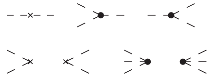
(a)

(b)

Figure 1: Diagrammatic representation of (a) the light-front Hamiltonian ${\cal P}^{-}$ and (b) the approximate $T$ operator for $\phi^{3}$ theory. The cross represents the kinetic energy contribution. External lines on the right represent annihilation operators; those on the left, creation operators.

The effective Hamiltonian $\overline{{\cal P}^{-}}$ of the LFCC method is computed from the Baker–Hausdorff expansion

$$\overline{{\cal P}^{-}}=e^{-T}{\cal P}^{-}e^{T}={\cal P}^{-}+[{\cal P}^{-},T]+\frac{1}{2!}[[{\cal P}^{-},T],T]+\cdots,$$ (11)

given an approximation for $T$.

To consider the lowest order zero-mode contribution, we truncate the $T$ operator to the creation of one zero mode

$$T=\int_{0}^{\infty}dp^{+}\sqrt{4\pi p^{+}}g(p^{+})a^{\dagger}(p^{+}),$$ (12)

with $g(p^{+})$ having support only at $p^{+}=0$ in a limit appropriate for the form chosen for $g$. For example, $g$ could be an exponential $\frac{1}{\epsilon}e^{-p^{+}/\epsilon}$ or a step function $\frac{1}{\epsilon}\theta(\epsilon-p^{+})$, with the appropriate limit being $\epsilon\rightarrow 0$. This limit, taken at the end of the calculation, restores momentum conservation. The valence state is the bare vacuum, and the projection $1-P_{v}$ is truncated to include only states with one zero mode. The corresponding transformation of the field is

$$e^{-T}\phi e^{T}=\phi+[\phi,T]+\cdots=\phi+\int dp^{+}g(p^{+})e^{-ip^{+}x^{-}/2},$$ (13)

which provides for a constant shift in the limit that $g(p^{+})\propto\delta(p^{+})$. A graphical representation of $T$ is given in Fig. 1.

A calculation of the terms in the Baker–Hausdorff expansion (11) then determines the effective Hamiltonian. Only a finite number of terms will contribute to the eigenvalue problem, because we need only terms that change the particle number by no more than one; any more than this would go beyond the truncation of the projection $(1-P_{v})$. We will consider only the vacuum as the valence state, and, therefore, terms in $\overline{{\cal P}^{-}}$ with any annihilation operators will also be neglected; however, such terms do need to be kept in intermediate calculations of commutators, because higher-order commutators can reduce the total number of annihilation operators.

We compute the following commutators for $T$ with ${\cal P}_{\rm free}^{-}$:

$$[{\cal P}_{\rm free}^{-},T] = \sqrt{4\pi}\mu^{2}\int dp^{+}\frac{g(p^{+})}{\sqrt{p^{+}}}a^{\dagger}(p^{+})$$

$$+\sqrt{4\pi}\mu^{2}\int\frac{dp_{1}^{+}dp_{2}^{+}}{\sqrt{p_{1}^{+}}}\delta(p_{1}^{+}+p_{2}^{+})g(p_{2}^{+})a(p_{1}^{+}),$$

$${[}[{\cal P}_{\rm free}^{-},T],T]=4\pi\mu^{2}\int dp_{1}^{+}dp_{2}^{+}\delta(p_{1}^{+}+p_{2}^{+})g(p_{1}^{+})g(p_{2}^{+}),$$ (15)

$${[}[[{\cal P}_{\rm free}^{-},T],T],T]=0,$$ (16)

and with ${\cal P}_{\rm int}^{-}$:

$${[}{\cal P}_{\rm int}^{-},T] = \lambda\int\frac{dp^{+}dp^{\prime+}}{\sqrt{p^{+}(p^{+}-p^{\prime+})}}g(p^{\prime+})a^{\dagger}(p^{+})a(p^{+}-p^{\prime+})$$

$$+\frac{\lambda}{2}\int\frac{dp^{+}dp^{\prime+}}{\sqrt{p^{+}(p^{+}-p^{\prime+})}}g(p^{+})a^{\dagger}(p^{\prime+})a^{\dagger}(p^{+}-p^{\prime+})$$

$$+\frac{\lambda}{2}\int\frac{dp_{1}^{+}dp_{2}^{+}dp_{3}^{+}}{\sqrt{p_{1}^{+}p_{2}^{+}}}\delta(p_{1}^{+}+p_{2}^{+}+p_{3}^{+})g(p_{3}^{+})a(p_{1}^{+})a(p_{2}^{+}),$$

$${[}[{\cal P}_{\rm int}^{-},T],T] = \sqrt{4\pi}\lambda\int\frac{dp^{+}dp^{\prime+}}{\sqrt{p^{+}}}g(p^{\prime+})g(p^{+}-p^{\prime+})a^{\dagger}(p^{+})$$

$$+\sqrt{4\pi}\lambda\int\frac{dp_{1}^{+}dp_{2}^{+}dp_{3}^{+}}{\sqrt{p_{1}^{+}}}\delta(p_{1}^{+}+p_{2}^{+}+p_{3}^{+})g(p_{2}^{+})g(p_{3}^{+})a(p_{1}^{+}),$$

$${[}[[{\cal P}_{\rm int}^{-},T],T],T]=4\pi\lambda\int dp_{1}^{+}dp_{2}^{+}dp_{3}^{+}\delta(p_{1}^{+}+p_{2}^{+}+p_{3}^{+})g(p_{1}^{+})g(p_{2}^{+})g(p_{3}^{+}),$$ (19)

$${[}[[[{\cal P}_{\rm int}^{-},T],T],T],T]=0.$$ (20)

Each commutator with ${\cal P}^{-}$ contracts one zero-mode creation operator with one annihilation operator in ${\cal P}^{-}$.

From these commutators we build the expression for $\overline{{\cal P}^{-}}$, keeping only those terms that do not annihilate the vacuum and create at most one zero mode. This gives

$$\overline{{\cal P}^{-}} = \sqrt{4\pi}\mu^{2}\int dp^{+}\frac{g(p^{+})}{\sqrt{p^{+}}}a^{\dagger}(p^{+})$$

$$+\frac{1}{2!}4\pi\mu^{2}\int dp_{1}^{+}dp_{2}^{+}\delta(p_{1}^{+}+p_{2}^{+})g(p_{1}^{+})g(p_{2}^{+})$$

$$+\frac{1}{2!}\sqrt{4\pi}\lambda\int\frac{dp^{+}dp^{\prime+}}{\sqrt{p^{+}}}g(p^{\prime+})g(p^{+}-p^{\prime+})a^{\dagger}(p^{+})$$

$$+\frac{1}{3!}4\pi\lambda\int dp_{1}^{+}dp_{2}^{+}dp_{3}^{+}\delta(p_{1}^{+}+p_{2}^{+}+p_{3}^{+})g(p_{1}^{+})g(p_{2}^{+})g(p_{3}^{+}).$$

A graphical representation is given in Fig. 2

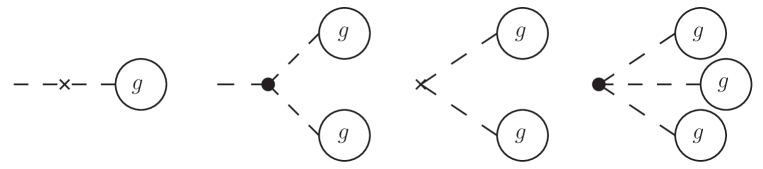
Figure 2: Same as Fig. 1, but for the zero-mode terms in the effective Hamiltonian $\overline{{\cal P}^{-}}$. Internal lines represent contractions.

For the vacuum valence state $|0\rangle$, the eigenvalue problem in the valence sector $P_{v}\overline{{\cal P}^{-}}|0\rangle=P^{-}|0\rangle$ is

$$\left[\frac{1}{2}4\pi\mu^{2}\int dp_{1}^{+}dp_{2}^{+}\delta(p_{1}^{+}+p_{2}^{+})g(p_{1}^{+})g(p_{2}^{+})\right.$$

$$\left.+\frac{1}{6}4\pi\lambda\int dp_{1}^{+}dp_{2}^{+}dp_{3}^{+}\delta(p_{1}^{+}+p_{2}^{+}+p_{3}^{+})g(p_{1}^{+})g(p_{2}^{+})g(p_{3}^{+})\right]|0\rangle=P^{-}|0\rangle.$$

If one assumes that $g$ is a function with support only at $p^{+}=0$, that is $g(p^{+})=\alpha\delta(p^{+})$, the eigenvalue $P^{-}$ is

$$P^{-}=\frac{1}{2}4\pi\mu^{2}\alpha^{2}\delta(0)+\frac{1}{6}4\pi\lambda\alpha^{3}\delta(0).$$ (23)

The $\delta(0)$ factors are no surprise, because we expect $P^{-}$ to be infinite, proportional to the volume

$$\lim_{p^{+}\rightarrow 0}\int dx^{-}e^{ip^{+}x^{-}/2}=\int dx^{-}=4\pi\delta(0).$$ (24)

Therefore, we write $P^{-}$ in terms of an energy density ${\cal E}^{-}$ as

$$P^{-}={\cal E}^{-}\int dx^{-},$$ (25)

and find

$${\cal E}^{-}=\frac{1}{2}\mu^{2}\alpha^{2}+\frac{1}{6}\lambda\alpha^{3}.$$ (26)

Clearly, the spectrum is unbounded from below Baym as $\alpha$ goes to negative infinity.

The form of the function $g$ was already assumed to be a delta function. Now let us see that this is exactly what the auxiliary equation (4) gives. Truncated to states with only one zero mode, the auxiliary equation becomes

$$\sqrt{4\pi}\mu^{2}\frac{g(p^{+})}{\sqrt{p^{+}}}+\frac{1}{2}\sqrt{4\pi}\lambda\int_{0}^{p^{+}}\frac{dp^{\prime+}}{\sqrt{p^{+}}}g(p^{\prime+})g(p^{+}-p^{\prime+})=0.$$ (27)

This equation can be solved by taking the Laplace transform after multiplication by $\sqrt{p^{+}}$. With the definition

$$G(s)\equiv\int_{0}^{\infty}e^{-sp^{+}}g(p^{+})dp^{+},$$ (28)

Eq. (27) becomes

$$\mu^{2}G(s)+\frac{1}{2}\lambda G(s)^{2}=0,$$ (29)

where the Laplace transform of the convolution in the second term is just the product of the transforms. The possible solutions are $G(s)$=0 and $-2\mu^{2}/\lambda$. Because the inverse transform of a constant is a delta function, we obtain the expected $g(p^{+})=\alpha\delta(p^{+})$ with $\alpha=0$ or $\alpha=-2\mu^{2}/\lambda$. These are the local extrema of ${\cal E}^{-}$; the LFCC auxiliary equation does miss the global extrema at $\pm\infty$.

This analysis leads to a natural choice for a limiting form to use in the construction of zero-mode $T$ operators. We define

$$\Delta(p^{+})=\frac{1}{\epsilon}e^{-p^{+}/\epsilon}$$ (30)

so that $\lim_{\epsilon\rightarrow 0}\Delta(p^{+})=\delta(p^{+})$, for integrals from zero to infinity, and the Laplace transform is

$$\int_{0}^{\infty}dp^{+}e^{-sp^{+}}\Delta(p^{+})=\frac{1}{\epsilon}\frac{1}{s+1/\epsilon}\rightarrow 1$$ (31)

For $\phi^{3}$ we would then define the truncated $T$ operator as

$$T=\alpha\int_{0}^{\infty}dp^{+}\sqrt{4\pi p^{+}}\Delta(p^{+})a^{\dagger}(p^{+}).$$ (32)

For comparison with the LFCC result, we consider a variational coherent-state analysis coherentstates of the light-front vacuum energy density $\langle\alpha|\!:\!{\cal H}\!:\!|\alpha\rangle$, with respect to a vacuum state $|\alpha\rangle$. This provides a direct correspondence with the LFCC result when, as above, the $T$ operator is truncated to one zero mode, because $|\alpha\rangle\equiv\sqrt{Z_{\alpha}}e^{T}|0\rangle$ is then a coherent state. With $T$ represented as in (32), the following commutators can be computed:

$${[}T^{\dagger},T] = 4\pi\alpha^{2}\int dp^{+}p^{+}\Delta^{2}(p^{+})\rightarrow\pi\alpha^{2},$$ (33)

$${[}\phi,T] = \alpha\int dp^{+}\Delta(p^{+})e^{-ip^{+}x^{-}/2}\rightarrow\alpha,$$ (34)

$${[}\phi,T^{\dagger}] = \alpha\int dp^{+}\Delta(p^{+})e^{+ip^{+}x^{-}/2}\rightarrow\alpha.$$ (35)

We then have, for real $\alpha$, $\sqrt{Z_{\alpha}}=e^{-\pi\alpha^{2}/2}$, $\phi|\alpha\rangle=\alpha|\alpha\rangle$, $\langle\alpha|\phi=\langle\alpha|\alpha$, and

$$\langle\alpha|\!:\!{\cal H}\!:\!|\alpha\rangle=\frac{1}{2}\mu^{2}\alpha^{2}+\frac{1}{6}\lambda\alpha^{3}={\cal E}^{-}.$$ (36)

The local extrema are at $\alpha=0$ and $\alpha=-2\mu^{2}/\lambda$, as in the LFCC analysis, and the global extrema at $\pm\infty$. The vacuum expectation value for the field is just $\langle\alpha|\phi|\alpha\rangle=\alpha$.

A different choice for the function $\Delta(p^{+})$ would change the result in (33) for the commutator $[T^{\dagger},T]$. For example, the step function $\frac{1}{\epsilon}\theta(\epsilon-p^{+})$ would yield

$$4\pi\alpha^{2}\int_{0}^{\epsilon}\frac{1}{\epsilon^{2}}p^{+}dp^{+}=2\pi\alpha^{2},$$ (37)

which differs by a factor of two. However, this changes the relative normalization $Z_{\alpha}$ but not the expectation value; the commutators $[\phi,T]$ and $[\phi,T^{\dagger}]$ are unaffected, because all forms of $\Delta(p^{+})$ must be consistent with $\delta(p^{+})$ as the limit.

IV $\phi^{4}$ theory

The Lagrangian and light-front Hamiltonian density for $\phi^{4}$ theory are

$${\cal L}=\frac{1}{2}(\partial_{\mu}\phi)^{2}-\frac{1}{2}\mu^{2}\phi^{2}-\frac{\lambda}{4!}\phi^{4}$$ (38)

and

$${\cal H}=\frac{1}{2}\mu^{2}\phi^{2}+\frac{\lambda}{4!}\phi^{4}.$$ (39)

The mode expansion for the field $\phi$ is the same as (7) for $\phi^{3}$ theory. We again split the light-front Hamiltonian ${\cal P}^{-}$ into two parts, ${\cal P}_{\rm free}^{-}$, which is given in Eq. (III), and

$${\cal P}_{\rm int}^{-} = \frac{\lambda}{6}\int\frac{dp_{1}^{+}dp_{2}^{+}dp_{3}^{+}}{4\pi\sqrt{p_{1}^{+}p_{2}^{+}p_{3}^{+}(p_{1}^{+}+p_{2}^{+}+p_{3}^{+})}}$$

$$\rule{72.26999pt}{0.0pt}\times\left[a^{\dagger}(p_{1}^{+}+p_{2}^{+}+p_{3}^{+})a(p_{1}^{+})a(p_{2}^{+})a(p_{3}^{+})\right.$$

$$\rule{90.3375pt}{0.0pt}\left.+a^{\dagger}(p_{1}^{+})a^{\dagger}(p_{2}^{+})a^{\dagger}(p_{3}^{+})a(p_{1}^{+}+p_{2}^{+}+p_{3}^{+})\right]$$

$$+\frac{\lambda}{4}\int\frac{dp_{1}^{+}dp_{2}^{+}}{4\pi\sqrt{p_{1}^{+}p_{2}^{+}}}\int\frac{dp_{1}^{\prime+}dp_{2}^{\prime+}}{\sqrt{p_{1}^{\prime+}p_{2}^{\prime+}}}\delta(p_{1}^{+}+p_{2}^{+}-p_{1}^{\prime+}-p_{2}^{\prime+})$$

$$\rule{144.54pt}{0.0pt}\times a^{\dagger}(p_{1}^{+})a^{\dagger}(p_{2}^{+})a(p_{1}^{\prime+})a(p_{2}^{\prime+})$$

$$+\frac{\lambda}{24}\int\frac{dp_{1}^{+}dp_{2}^{+}dp_{3}^{+}dp_{4}^{+}}{4\pi\sqrt{p_{1}^{+}p_{2}^{+}p_{3}^{+}p_{4}^{+}}}\delta(p_{1}^{+}+p_{2}^{+}+p_{3}^{+}+p_{4}^{+})$$

$$\rule{36.135pt}{0.0pt}\times\left[a^{\dagger}(p_{1}^{+})a^{\dagger}(p_{2}^{+})a^{\dagger}(p_{3}^{+})a^{\dagger}(p_{4}^{+})+a(p_{1}^{+})a(p_{2}^{+})a(p_{3}^{+})a(p_{4}^{+})\right].$$

A graphical representation is shown in Fig. 3.

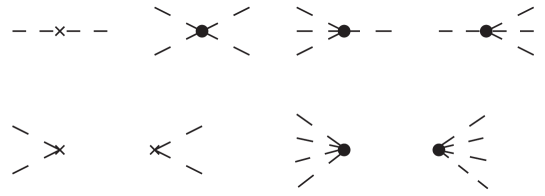
(a)

(b)

Figure 3: Same as Fig. 1, but for $\phi^{4}$ theory.

We focus on the zero-mode contributions to a vacuum valence state and consider the $T$ operator (32) for a single zero mode. The variational coherent-state approach gives

$$\langle\alpha|\!:\!{\cal H}\!:\!|\alpha\rangle=\frac{1}{2}\mu^{2}\alpha^{2}+\frac{1}{24}\lambda\alpha^{4},$$ (41)

with a local maximum at $\alpha=0$ and local minima at $\alpha^{2}=-6\mu^{2}/\lambda$. Of course, the latter is realizable only for $\mu^{2}<0$.

For the LFCC analysis, the relevant commutators with ${\cal P}_{\rm free}^{-}$ are the same as those for $\phi^{3}$ theory, with $g(p^{+})=\alpha\Delta(p^{+})$, given in Eqs. (III) and (15). Those for ${\cal P}_{\rm int}^{-}$ are

$${[}{\cal P}_{\rm int}^{-},T] = \frac{\lambda\alpha}{2}\int\frac{dp_{1}^{+}dp_{2}^{+}dp^{+}}{\sqrt{4\pi p_{1}^{+}p_{2}^{+}p^{+}}}\delta(p^{+}-p_{1}^{+}-p_{2}^{+})$$

$$\rule{36.135pt}{0.0pt}\times\left[a^{\dagger}(p^{+})a(p_{1}^{+})a(p_{2}^{+})+a^{\dagger}(p_{1}^{+})a^{\dagger}(p_{2}^{+})a(p^{+})\right]$$

$$+\frac{\lambda\alpha}{6}\int\frac{dp_{1}^{+}dp_{2}^{+}dp_{3}^{+}}{\sqrt{4\pi p_{1}^{+}p_{2}^{+}p_{3}^{+}}}\delta(p_{1}^{+}+p_{2}^{+}+p_{3}^{+})$$

$$\rule{36.135pt}{0.0pt}\times\left[a(p_{1}^{+})a(p_{2}^{+})a(p_{3}^{+})+a^{\dagger}(p_{1}^{+})a^{\dagger}(p_{2}^{+})a^{\dagger}(p_{3}^{+}\right],$$

$${[}[{\cal P}_{\rm int}^{-},T],T] = \lambda\alpha^{2}\int\frac{dp^{+}}{p^{+}}a^{\dagger}(p^{+})a(p^{+})$$

$$+\frac{\lambda\alpha^{2}}{2}\int\frac{dp_{1}^{+}dp_{2}^{+}}{\sqrt{p_{1}^{+}p_{2}^{+}}}\delta(p_{1}^{+}+p_{2}^{+})\left[a(p_{1}^{+})a(p_{2}^{+})+a^{\dagger}(p_{1}^{+})a^{\dagger}(p_{2}^{+})\right],$$

$${[}[[{\cal P}_{\rm int}^{-},T],T],T]=\sqrt{4\pi}\lambda\alpha^{3}\int\frac{dp^{+}}{\sqrt{p^{+}}}\Delta(p^{+})\left[a(p^{+})+a^{\dagger}(p^{+})\right],$$ (44)

$${[}[[[{\cal P}_{\rm int}^{-},T],T],T],T]=4\pi\lambda\alpha^{4}\delta(0),$$ (45)

$${[}[[[[{\cal P}_{\rm int}^{-},T],T],T],T],T]=0.$$ (46)

From these commutators we construct the effective Hamiltonian, keeping only terms which do not annihilate the vacuum and do not add more than one zero mode,

$$\overline{{\cal P}^{-}} = \sqrt{4\pi}\left[\mu^{2}\alpha+\frac{1}{6}\lambda\alpha^{3}\right]\int\frac{dp^{+}}{\sqrt{p^{+}}}\Delta(p^{+})a^{\dagger}(p^{+})$$

$$+4\pi\left[\frac{1}{2}\mu^{2}\alpha^{2}+\frac{1}{24}\lambda\alpha^{4}\right]\delta(0).$$

Figure 4 provides a graphical representation.

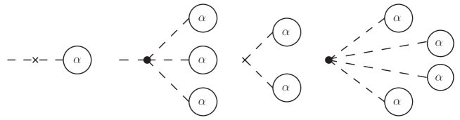
Figure 4: Same as Fig. 2, but for $\phi^{4}$ theory.

For a vacuum valence state, the valence eigenvalue problem is

$$P_{v}\overline{{\cal P}^{-}}|0\rangle={\cal E}^{-}\int dx^{-}|0\rangle,$$ (48)

with

$${\cal E}^{-}=\frac{1}{2}\mu^{2}\alpha^{2}+\frac{1}{24}\lambda\alpha^{4}.$$ (49)

The auxiliary equation (4), projected onto the one-zero-mode sector, yields

$$\mu^{2}\alpha+\frac{1}{6}\lambda\alpha^{3}=0.$$ (50)

These provide a complete match with the coherent-state result (41), with $\alpha=0$ or $\alpha^{2}=-6\mu^{2}/\lambda$, and $\alpha$ the vacuum expectation value for the field.

If we now consider the wrong-sign case, with $\mu^{2}\rightarrow-\mu^{2}$, we find $\alpha=\pm\sqrt{6\lambda}/\mu$, which corresponds to the shift of the field $\phi$ that brings the energy density to a minimum. Thus, the inclusion of a zero mode in the LFCC $T$ operator allows for the necessary shift in the field. Also, as can be seen from the commutator in (IV), the effective Hamiltonian will have terms that change the particle number by one and thereby mix Fock states with odd and even numbers of particles, which is characteristic of broken symmetry.

V Wick–Cutkosky model

To illustrate what happens in a more complicated theory, we consider the Wick–Cutkosky model WC of a charged scalar coupled to a neutral scalar. The Lagrangian is

$${\cal L}=\frac{1}{2}(\partial_{\mu}\phi)^{2}-\frac{1}{2}\mu^{2}\phi^{2}+|\partial_{\mu}\chi|^{2}-m^{2}\chi^{2}-g\phi|\chi|^{2},$$ (51)

where $\phi$ is the neutral scalar field and $\chi$ the complex charged scalar field. The Hamiltonian density is

$${\cal H}=\frac{1}{2}\mu^{2}\phi^{2}+m^{2}|\chi|^{2}+g\phi|\chi|^{2}.$$ (52)

The mode expansion for the field $\phi$ is the same as (7) for $\phi^{3}$ theory; the mode expansion for $\chi$ is

$$\chi=\int\frac{dp^{+}}{\sqrt{4\pi p^{+}}}\left\{c_{+}(p^{+})e^{-ip^{+}x^{-}/2}+c_{-}^{\dagger}(p^{+})e^{ip^{+}x^{-}/2}\right\},$$ (53)

with $c^{\dagger}_{\pm}$ the creation operator for the positive (negative) charge. The nonzero commutation relation is

$$[c_{\pm}(p^{+}),c_{\pm}^{\dagger}(p^{\prime+})]=\delta(p^{+}-p^{\prime+}).$$ (54)

The free and interacting parts of the light-front Hamiltonian ${\cal P}^{-}$ are

$${\cal P}_{\rm free}^{-}={\cal P}_{\phi\rm free}^{-}+{\cal P}_{\chi\rm free}^{-}$$ (55)

with ${\cal P}_{\phi\rm free}^{-}$ the free part for the $\phi$ field, as given in (III),

$${\cal P}_{\chi\rm free}^{-} = \int dp^{+}\frac{m^{2}}{p^{+}}\left[c_{+}^{\dagger}(p^{+})c_{+}(p^{+})+c_{-}^{\dagger}(p^{+})c_{-}(p^{+})\right]$$

$$+m^{2}\int\frac{dp_{1}^{+}dp_{2}^{+}}{\sqrt{p_{1}^{+}p_{2}^{+}}}\delta(p_{1}^{+}+p_{2}^{+})\left[c_{+}^{\dagger}(p_{1}^{+})c_{-}^{\dagger}(p_{2}^{+})+c_{+}(p_{1}^{+})c_{-}(p_{2}^{+})\right],$$

and

$${\cal P}_{\rm int}^{-} = g\int\frac{dp_{1}^{+}dp_{2}^{+}dp_{3}^{+}}{\sqrt{4\pi p_{1}^{+}p_{2}^{+}p_{3}^{+}}}\delta(p_{1}^{+}+p_{2}^{+}+p_{3}^{+})$$

$$\rule{36.135pt}{0.0pt}\times\left[a^{\dagger}(p_{1}^{+})c_{+}^{\dagger}(p_{2}^{+})c_{-}^{\dagger}(p_{3}^{+})+a(p_{1}^{+})c_{+}(p_{2}^{+})c_{-}(p_{3}^{+})\right]$$

$$+g\int\frac{dp_{1}^{+}dp_{2}^{+}}{\sqrt{4\pi p_{1}^{+}p_{2}^{+}(p_{1}^{+}+p_{2}^{+})}}\left\{a^{\dagger}(p_{1}^{+}+p_{2}^{+})c_{+}(p_{1}^{+})c_{-}(p_{2}^{+})\right.$$

$$\rule{36.135pt}{0.0pt}+a^{\dagger}(p_{1}^{+})\left[c_{+}^{\dagger}(p_{2}^{+})c_{+}(p_{1}^{+}+p_{2}^{+})+c_{-}^{\dagger}(p_{2}^{+})c_{-}(p_{1}^{+}+p_{2}^{+})\right]$$

$$\rule{36.135pt}{0.0pt}+\left[c_{+}^{\dagger}(p_{1}^{+}+p_{2}^{+})c_{+}(p_{2}^{+})+c_{-}^{\dagger}(p_{1}^{+}+p_{2}^{+})c_{-}(p_{2}^{+})\right]a(p_{1}^{+})$$

$$\rule{36.135pt}{0.0pt}\left.+c_{+}^{\dagger}(p_{1}^{+})c_{-}^{\dagger}(p_{2}^{+})a(p_{1}^{+}+p_{2}^{+})\right\}.$$

A graphical representation is given in Fig. 5.

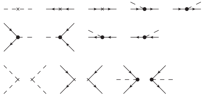
(a)

(b)

Figure 5: Same as Fig. 1, but for the Wick–Cutkosky model. The charged scalars are represented by solid lines, with the arrow to the left (right) for positive (negative) charge; the neutral scalars are represented by dashed lines. The zero-mode contributions are labeled by $\alpha$ for the neutral scalar and by $h$ for the charged pair.

We again focus on the zero-mode contributions and consider the $T$ operator

$$T=T_{\phi}+T_{\chi},$$ (58)

with $T_{\phi}$ defined as in (32) and

$$T_{\chi}=\int dp_{1}^{+}dp_{2}^{+}4\pi\sqrt{p_{1}^{+}p_{2}^{+}}h(p_{1}^{+},p_{2}^{+})c_{+}^{\dagger}(p_{1}^{+})c_{-}^{\dagger}(p_{2}^{+}).$$ (59)

The first term, $T_{\phi}$, creates a neutral-scalar zero mode; the second creates a neutral pair of charged zero modes. The function $h$ is to be determined from the LFCC equations, but can be assumed to be symmetric: $h(p_{1}^{+},p_{2}^{+})=h(p_{2}^{+},p_{1}^{+})$. The first term in $T$ again corresponds to a shift of the field $\phi$ by a constant $\alpha$.

The relevant commutators with ${\cal P}^{-}$ are given in A. These yield an effective Hamiltonian of

$$\overline{{\cal P}^{-}}=\sqrt{4\pi}\alpha\mu^{2}\int dp^{+}\frac{\Delta(p^{+})}{\sqrt{p^{+}}}a^{\dagger}(p^{+})+\frac{1}{2}\alpha^{2}\mu^{2}\int dx^{-}$$

$$+\sqrt{4\pi}g\int\frac{dp_{1}^{+}dp_{2}^{+}}{\sqrt{p_{1}^{+}+p_{2}^{+}}}h(p_{1}^{+},p_{2}^{+})a^{\dagger}(p_{1}^{+}+p_{2}^{+})$$

$$+(m^{2}+\alpha g)\int dp_{1}^{+}dp_{2}^{+}\left\{\rule{0.0pt}{18.06749pt}4\pi\delta(p_{1}^{+}+p_{2}^{+})h(p_{1}^{+},p_{2}^{+})\right.$$

$$\rule{36.135pt}{0.0pt}+\frac{1}{\sqrt{p_{1}^{+}p_{2}^{+}}}\left[\delta(p_{1}^{+}+p_{2}^{+})+4\pi(p_{1}^{+}+p_{2}^{+})h(p_{1}^{+},p_{2}^{+})\right]c_{+}^{\dagger}(p_{1}^{+})c_{-}^{\dagger}(p_{2}^{+})$$

$$\rule{36.135pt}{0.0pt}+(4\pi)^{2}\delta(p_{1}^{+}+p_{2}^{+})\int dp_{1}^{\prime+}dp_{2}^{\prime+}\sqrt{p_{1}^{\prime+}p_{2}^{\prime+}}$$

$$\rule{144.54pt}{0.0pt}\left.\times h(p_{1}^{+},p_{2}^{\prime+})h(p_{2}^{+},p_{1}^{\prime+})c_{+}^{\dagger}(p_{1}^{\prime+})c_{-}^{\dagger}(p_{2}^{\prime+})\rule{0.0pt}{18.06749pt}\right\},$$

where we list only those terms that do not annihilate the Fock vacuum and do not create more than one neutral zero mode or one pair of charged zero modes. Figure 6 shows a graphical representation.

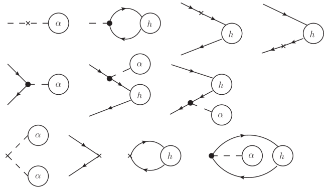
Figure 6: Same as Fig. 5, but for the zero-mode terms in the effective Hamiltonian $\overline{{\cal P}^{-}}$.

In the vacuum valence sector, the eigenvalue problem $P_{v}\overline{{\cal P}^{-}}|0\rangle=P^{-}|0\rangle$ determines $P^{-}$ to be

$$P^{-}=\frac{1}{2}\alpha^{2}\mu^{2}\int dx^{-}+4\pi(m^{2}+\alpha g)\int dp_{1}^{+}dp_{2}^{+}\delta(p_{1}^{+}+p_{2}^{+})h(p_{1}^{+},p_{2}^{+}).$$ (61)

To have enough equations to solve for the unknowns $\alpha$ and $h(p_{1}^{+},p_{2}^{+})$ in the $T$ operator, we must project the auxiliary equation (4) onto the Fock sector with one neutral zero mode and onto the sector with a neutral pair. These projections yield

$$\alpha\mu^{2}\frac{\Delta(p^{+})}{\sqrt{p^{+}}}+g\int_{0}^{p^{+}}\frac{dp^{\prime+}}{\sqrt{p^{+}}}h(p^{\prime+},p^{+}-p^{\prime+})=0$$ (62)

and

$$(m^{2}+\alpha g)\left[\frac{\delta(p_{1}^{+}+p_{2}^{+})}{\sqrt{p_{1}^{+}p_{2}^{+}}}+4\pi\frac{p_{1}^{+}+p_{2}^{+}}{\sqrt{p_{1}^{+}p_{2}^{+}}}h(p_{1}^{+},p_{2}^{+})\right.$$

$$\left.+(4\pi)^{2}\int dp_{1}^{\prime+}dp_{2}^{\prime+}\delta(p_{1}^{\prime+}+p_{2}^{\prime+})\sqrt{p_{1}^{+}p_{2}^{+}}h(p_{1}^{\prime+},p_{2}^{+})h(p_{2}^{\prime+},p_{1}^{+})\rule{0.0pt}{21.68121pt}\right]=0.$$

The last term in (V) is actually zero, as can be seen from the change of integration variables to $P^{\prime+}=p_{1}^{\prime+}+p_{2}^{\prime+}$ and $x^{\prime}=p_{1}^{\prime+}/P^{\prime+}$. The integrals in this term then take the form

$$\int P^{\prime+}dx^{\prime}dP^{\prime+}\delta(P^{\prime+})h(x^{\prime}P^{\prime+},p_{2}^{+})h((1-x^{\prime})P^{\prime+},p_{1}^{+}),$$ (64)

which is proportional to $\int P^{\prime+}\delta(P^{\prime+})dP^{\prime+}=0$.

To solve these equations, we consider two cases, one where $m^{2}+\alpha g$ is not zero and the other where it is. For $m^{2}+\alpha g\neq 0$, we have, from (V)

$$h(p_{1}^{+},p_{2}^{+})=-\frac{\delta(p_{1}^{+}+p_{2}^{+})}{4\pi(p_{1}^{+}+p_{2}^{+})}\longrightarrow-\frac{\Delta(p_{1}^{+}+p_{2}^{+})}{4\pi(p_{1}^{+}+p_{2}^{+})}.$$ (65)

Substitution into (62) yields

$$\alpha\mu^{2}\frac{\Delta(p^{+})}{\sqrt{p^{+}}}-g\frac{\Delta(p^{+})}{\sqrt{p^{+}}}\int_{0}^{p^{+}}\frac{dp^{\prime+}}{4\pi p^{+}}=0$$ (66)

or

$$\alpha=\frac{g}{4\pi\mu^{2}}.$$ (67)

We can also obtain an explicit form for the eigenvalue $P^{-}={\cal E}^{-}\int dx^{-}$ from (61), with use of the same change of variables in the integration

$$\int dp_{1}^{+}dp_{2}^{+}\delta(p_{1}^{+}+p_{2}^{+})h(p_{1}^{+},p_{2}^{+}) = -\int P^{+}dxdP^{+}\delta(P^{+})\frac{\delta(P^{+})}{4\pi P^{+}}$$

$$= \frac{-1}{4\pi}\delta(0)=\frac{-1}{(4\pi)^{2}}\int dx^{-}.$$

This leaves

$${\cal E}^{-}=\frac{1}{2}\alpha^{2}\mu^{2}-\frac{1}{4\pi}(m^{2}+\alpha g)=-\frac{1}{4\pi}\left(m^{2}+\frac{g^{2}}{8\pi\mu^{2}}\right).$$ (69)

When $m^{2}+\alpha g=0$, we obviously have

$$\alpha=-\frac{m^{2}}{g}.$$ (70)

From (61), we see that

$${\cal E}^{-}=\frac{1}{2}\alpha^{2}\mu^{2}=\frac{1}{2}\frac{m^{4}\mu^{2}}{g^{2}},$$ (71)

independent of the form of $h(p_{1}^{+},p_{2}^{+})$. The function $h$ does still help determine the vacuum state and must still satisfy (62), which becomes

$$\int_{0}^{p^{+}}dp^{\prime+}h(p^{\prime+},p^{+}-p^{\prime+})=\frac{m^{2}\mu^{2}}{g^{2}}\Delta(p^{+}).$$ (72)

With a change of variable to $x^{\prime}\equiv p^{\prime+}/p^{+}$, we obtain

$$\int_{0}^{1}dx^{\prime}h(x^{\prime}p^{+},(1-x^{\prime})p^{+})=\frac{m^{2}\mu^{2}}{g^{2}}\frac{\Delta(p^{+})}{p^{+}}.$$ (73)

Therefore, $h(x^{\prime}p^{+},(1-x^{\prime})p^{+})$ is proportional to $\Delta(p^{+})/p^{+}$ and generally takes the form

$$h(p_{1}^{+},p_{2}^{+})=\frac{m^{2}\mu^{2}}{g^{2}}f\left(\frac{p_{1}^{+}}{p_{1}^{+}+p_{2}^{+}}\right)\frac{\Delta(p_{1}^{+}+p_{2}^{+})}{p_{1}^{+}+p_{2}^{+}},$$ (74)

with $f$ any function that satisfies $\int_{0}^{1}f(x)dx=1$. In the limit that $\Delta(p^{+})\rightarrow\delta(p^{+})$, the form of $f$ is irrelevant.

From the form of $P^{-}$ in (61), we see that, as expected for a cubic theory Baym , the spectrum is unbounded from below. However, as in the case of $\phi^{3}$ theory, the LFCC auxiliary equations determine only local extrema.

VI Summary

We have considered various examples of two-dimensional scalar theories where zero modes can play a role in the calculation of light-front Hamiltonian eigenstates. In each case, the LFCC method is able to incorporate the zero modes in a sensible way and, where it can be compared with a coherent-state analysis, obtains equivalent results for the local extrema of the energy density and the vacuum expectation value for the bosonic field. To do this, the $T$ operator must include terms that allow creation of modes with infinitesimal longitudinal momentum, with the limit of zero momentum taken at a later stage in the calculation. The vacuum state is then a generalized coherent state of zero modes, created from the trivial Fock vacuum by the operator $e^{T}$.

Although the examples are limited to two dimensions, there is no particular restriction on a direct extension to three or four dimensions. The zero-mode terms would include a dependence on transverse momenta.

With these tools in place, one can use the LFCC method to explore symmetry breaking nonperturbatively. A calculation in $\phi^{4}$ theory that includes as many as four zero modes in the $T$ operator should be sufficient to compute the critical coupling for dynamical symmetry breaking; this would parallel the calculations done in equal-time quantization CC-QFT . Another accessible application is a nonperturbative calculation of the Higgs mechanism and the associated breaking of a continuous symmetry. The general aim is, of course, to apply these methods to the nonperturbative solution of QCD in terms of hadronic wave functions, particularly with respect to symmetry-breaking effects.

Appendix A Commutators for the Wick–Cutkosky model

The commutators needed to construct the effective Hamiltonian for the Wick–Cutkosky model are below, with ${\cal P}_{\rm free}^{-}$ defined in (55), ${\cal P}_{\rm int}^{-}$ in (V), and $T$ in (58). The commutators of ${\cal P}_{\phi\rm free}^{-}$ with $T_{\phi}$ are the same as those for $\phi^{3}$ theory, with $g(p^{+})=\alpha\Delta(p^{+})$, given in Eqs. (III) and (15). The other commutators are

$$[{\cal P}_{\chi\rm free}^{-},T_{\chi}] = 4\pi m^{2}\int dp_{1}^{+}dp_{2}^{+}\left\{\rule{0.0pt}{21.68121pt}\delta(p_{1}^{+}+p_{2}^{+})h(p_{1}^{+},p_{2}^{+})\right.$$

$$+\frac{p_{1}^{+}+p_{2}^{+}}{\sqrt{p_{1}^{+}p_{2}^{+}}}h(p_{1}^{+},p_{2}^{+})c_{+}^{\dagger}(p_{1}^{+})c_{-}^{\dagger}(p_{2}^{+})$$

$$+\delta(p_{1}^{+}+p_{2}^{+})\int dp^{\prime+}\left[\sqrt{\frac{p^{\prime+}}{p_{1}^{+}}}h(p^{\prime+},p_{2}^{+})c_{+}^{\dagger}(p^{\prime+})c_{+}(p_{1}^{+})\right.$$

$$\left.\left.\rule{86.72377pt}{0.0pt}+\sqrt{\frac{p^{\prime+}}{p_{2}^{+}}}h(p_{1}^{+},p^{\prime+})c_{-}^{\dagger}(p^{\prime+})c_{-}(p_{2}^{+})\right]\right\},$$

$$[[{\cal P}_{\chi\rm free}^{-},T_{\chi}],T_{\phi}]=0,$$ (76)

$$[[{\cal P}_{\chi\rm free}^{-},T_{\phi}],T_{\chi}]=0,$$ (77)

$$[[{\cal P}_{\chi\rm free}^{-},T_{\chi}],T_{\chi}] = 2(4\pi)^{2}m^{2}\int dp_{1}^{+}dp_{2}^{+}\delta(p_{1}^{+}+p_{2}^{+})\int dp_{1}^{\prime+}dp_{2}^{\prime+}$$

$$\times\sqrt{p_{1}^{\prime+}p_{2}^{\prime+}}h(p_{1}^{+},p_{2}^{\prime+})h(p_{2}^{+},p_{1}^{\prime+})c_{+}^{\dagger}(p_{1}^{\prime+})c_{-}^{\dagger}(p_{2}^{\prime+}),$$

$$[[[{\cal P}_{\chi\rm free}^{-},T_{\chi}],T_{\chi}],T_{\chi}]=0,$$ (79)

$$[{\cal P}_{\rm int}^{-},T_{\phi}]=\frac{\alpha g}{m^{2}}{\cal P}_{\chi\rm free}^{-},$$ (80)

$$[[{\cal P}_{\rm int}^{-},T_{\phi}],T]=\frac{\alpha g}{m^{2}}[{\cal P}_{\chi\rm free}^{-},T_{\chi}],$$ (81)

$$[[[{\cal P}_{\rm int}^{-},T_{\phi}],T],T]=\frac{\alpha g}{m^{2}}[[{\cal P}_{\chi\rm free}^{-},T_{\chi}],T_{\chi}],$$ (82)

$$[[[[{\cal P}_{\rm int}^{-},T_{\phi}],T],T],T]=0,$$ (83)

$$[{\cal P}_{\rm int}^{-},T_{\chi}]=g\sqrt{4\pi}\int dp_{1}^{+}dp_{2}^{+}dp_{3}^{+}\delta(p_{1}^{+}+p_{2}^{+}+p_{3}^{+})\left[\rule{0.0pt}{21.68121pt}h(p_{2}^{+},p_{3}^{+})\right.$$

$$\rule{72.26999pt}{0.0pt}+\int dp_{1}^{\prime+}\sqrt{\frac{p_{1}^{\prime+}}{p_{2}^{+}}}h(p_{1}^{\prime+},p_{3}^{+})c_{+}^{\dagger}(p_{1}^{\prime+})c_{+}(p_{2}^{+})$$

$$\left.\rule{72.26999pt}{0.0pt}+\int dp_{2}^{\prime+}\sqrt{\frac{p_{2}^{\prime+}}{p_{3}^{+}}}h(p_{2}^{+},p_{2}^{\prime+})c_{-}^{\dagger}(p_{2}^{\prime+})c_{-}(p_{3}^{+})\right]\frac{a(p_{1}^{+})}{\sqrt{p_{1}^{+}}}$$

$$+g\sqrt{4\pi}\int dp_{1}^{+}dp_{2}^{+}\left\{\frac{h(p_{1}^{+},p_{2}^{+})}{\sqrt{p_{1}^{+}+p_{2}^{+}}}a^{\dagger}(p_{1}^{+}+p_{2}^{+})\right.$$

$$\rule{36.135pt}{0.0pt}+\int dp_{2}^{\prime+}\sqrt{\frac{p_{2}^{\prime+}}{p_{1}^{+}p_{2}^{+}}}h(p_{1}^{+}+p_{2}^{+},p_{2}^{\prime+})a^{\dagger}(p_{1}^{+})c_{+}^{\dagger}(p_{2}^{+})c_{-}^{\dagger}(p_{2}^{\prime+})$$

$$\rule{36.135pt}{0.0pt}+\int dp_{1}^{\prime+}\sqrt{\frac{p_{1}^{\prime+}}{p_{1}^{+}p_{2}^{+}}}h(p_{1}^{+}+p_{2}^{+},p_{1}^{\prime+})a^{\dagger}(p_{1}^{+})c_{+}^{\dagger}(p_{1}^{\prime+})c_{-}^{\dagger}(p_{2}^{+})$$

$$\rule{36.135pt}{0.0pt}+\int dp_{2}^{\prime+}\sqrt{\frac{p_{2}^{\prime+}}{p_{1}^{+}(p_{1}^{+}+p_{2}^{+})}}h(p_{2}^{+},p_{2}^{\prime+})c_{+}^{\dagger}(p_{1}^{+}+p_{2}^{+})c_{-}^{\dagger}(p_{2}^{\prime+})a(p_{1}^{+})$$

$$\rule{36.135pt}{0.0pt}+\int dp_{1}^{\prime+}\sqrt{\frac{p_{1}^{\prime+}}{p_{1}^{+}(p_{1}^{+}+p_{2}^{+})}}h(p_{2}^{+},p_{1}^{\prime+})c_{+}^{\dagger}(p_{1}^{\prime+})c_{-}^{\dagger}(p_{1}^{+}+p_{2}^{+})a(p_{1}^{+})$$

$$\rule{36.135pt}{0.0pt}+\int dp_{1}^{\prime+}\sqrt{\frac{p_{1}^{\prime+}}{p_{1}^{+}(p_{1}^{+}+p_{2}^{+})}}h(p_{2}^{+},p_{1}^{\prime+})a^{\dagger}(p_{1}^{+}+p_{2}^{+})c_{+}^{\dagger}(p_{1}^{\prime+})c_{+}(p_{1}^{+})$$

$$\rule{36.135pt}{0.0pt}\left.+\int dp_{2}^{\prime+}\sqrt{\frac{p_{2}^{\prime+}}{p_{2}^{+}(p_{1}^{+}+p_{2}^{+})}}h(p_{1}^{+},p_{2}^{\prime+})a^{\dagger}(p_{1}^{+}+p_{2}^{+})c_{-}^{\dagger}(p_{2}^{\prime+})c_{-}(p_{2}^{+})\right\},$$

$$[[{\cal P}_{\rm int}^{-},T_{\chi}],T_{\phi}] = 4\pi g\alpha\int dp_{2}^{+}dp_{3}^{+}\delta(p_{2}^{+}+p_{3}^{+})\left\{\rule{0.0pt}{21.68121pt}h(p_{2}^{+},p_{3}^{+})\right.$$

$$\rule{18.06749pt}{0.0pt}+\int dp_{1}^{+}\sqrt{\frac{p_{1}^{+}}{p_{2}^{+}}}h(p_{1}^{+},p_{3}^{+})\left[c_{+}^{\dagger}(p_{1}^{+})c_{+}(p_{2}^{+})\right.$$

$$\rule{144.54pt}{0.0pt}\left.\left.+c_{-}^{\dagger}(p_{1}^{+})c_{-}(p_{2}^{+})\right]\rule{0.0pt}{21.68121pt}\right\}$$

$$+4\pi g\alpha\int dp_{1}^{+}dp_{2}^{+}\frac{p_{1}^{+}+p_{2}^{+}}{\sqrt{p_{1}^{+}p_{2}^{+}}}h(p_{1}^{+},p_{2}^{+})c_{+}^{\dagger}(p_{1}^{+})c_{-}^{\dagger}(p_{2}^{+}),$$

$$[[{\cal P}_{\rm int}^{-},T_{\chi}],T_{\chi}] = 2g(4\pi)^{3/2}\int dp_{1}^{+}dp_{2}^{+}dp_{3}^{+}\delta(p_{1}^{+}+p_{2}^{+}+p_{3}^{+})$$

$$\int dp_{1}^{\prime+}dp_{2}^{\prime+}\sqrt{\frac{p_{1}^{\prime+}p_{2}^{\prime+}}{p_{1}^{+}}}$$

$$\rule{36.135pt}{0.0pt}\times h(p_{1}^{\prime+},p_{3}^{+})h(p_{2}^{\prime+},p_{2}^{+})c_{+}^{\dagger}(p_{1}^{\prime+})c_{-}^{\dagger}(p_{2}^{\prime+})a(p_{1}^{+})$$

$$+2g(4\pi)^{3/2}\int\frac{dp_{1}^{+}dp_{2}^{+}}{\sqrt{p_{1}^{+}+p_{2}^{+}}}\int dp_{1}^{\prime+}dp_{2}^{\prime+}\sqrt{p_{1}^{\prime+}p_{2}^{\prime+}}$$

$$\rule{36.135pt}{0.0pt}\times h(p_{1}^{+},p_{2}^{\prime+})h(p_{2}^{+},p_{1}^{\prime+})a^{\dagger}(p_{1}^{+}+p_{2}^{+})c_{+}^{\dagger}(p_{1}^{\prime+})c_{-}^{\dagger}(p_{2}^{\prime+}),$$

$$[[[{\cal P}_{\rm int}^{-},T_{\chi}],T_{\phi}],T_{\chi}] = [[[{\cal P}_{\rm int}^{-},T_{\chi}],T_{\chi}],T_{\phi}]$$ (87)

$$= 2g\alpha(4\pi)^{2}\int dp_{1}^{+}dp_{2}^{+}dp_{3}^{+}\delta(p_{2}^{+}+p_{3}^{+})$$

$$\int dp_{2}^{\prime+}\sqrt{p_{1}^{+}p_{2}^{\prime+}}h(p_{1}^{+},p_{3}^{+})h(p_{2}^{+},p_{2}^{\prime+})c_{+}^{\dagger}(p_{1}^{+})c_{-}^{\dagger}(p_{2}^{\prime+}),$$

and

$$[[[[{\cal P}_{\rm int}^{-},T_{\chi}],T_{\phi}],T_{\chi}],T]=0.$$ (89)

These are then combined according to the Baker–Hausdorff expansion to construct the effective Hamiltonian.

References

(1) P.A.M. Dirac,
Rev. Mod. Phys. 21 (1949), 392.
(2) For reviews of light-cone quantization, see
M. Burkardt, Adv. Nucl. Phys. 23 (2002), 1;
S.J. Brodsky, H.-C. Pauli, and S.S. Pinsky,
Phys. Rep. 301 (1998), 299.
(3) Th. Heinzl, St. Krusche, and E. Werner,
Phys. Lett. B 272 (1991), 54; 275 (1992), 410;
T. Heinzl, S. Krusche, S. Simburger, and E. Werner,
Z. Phys. C 56 (1992), 415.
(4) D.G. Robertson,
Phys. Rev. D 47 (1993), 2549.
(5) K. Hornbostel,
Phys. Rev. D 45 (1992), 3781.
(6) C.M. Bender, S.S. Pinsky, and B. van de Sande,
Phys. Rev. D 48 (1993), 816;
S.S. Pinsky and B. van de Sande, Phys. Rev. D 49 (1994), 2001;
S.S. Pinsky, B. van de Sande, and J.R. Hiller,
Phys. Rev. D 51 (1995), 726.
(7)
A. Borderies, P. Grangé, and E. Werner,
Phys. Lett. B 319 (1993), 490; 345 (1995), 458;
P. Grangé, P. Ullrich, and E. Werner, Phys. Rev. D 57 (1998), 4981;
S. Salmons, P. Grangé, and E. Werner, Phys. Rev. D 60 (1999), 067701;
S. Salmons, P. Grangé, and E. Werner,
Phys. Rev. D 65 (2002), 125014.
(8) J.S. Rozowsky and C.B. Thorn,
Phys. Rev. Lett. 85 (2000), 1614.
(9) V. T. Kim, G. B. Pivovarov, and J. P. Vary,
Phys. Rev. D 69 (2004), 085008;
D. Chakrabarti, A. Harindranath, L. Martinovic, and J.P. Vary,
Phys. Lett. B 582 (2004), 196;
D. Chakrabarti, A. Harindranath, L. Martinovic,
G.B. Pivovarov, and J.P. Vary,
Phys. Lett. B 617 (2005), 92;
D. Chakrabarti, A. Harindranath, and J.P. Vary,
Phys. Rev. D 71 (2005), 125012.
(10) S.S. Chabysheva and J.R. Hiller,
Phys. Rev. D 79 (2009), 096012.
(11) T. Maskawa and K. Yamawaki,
Prog. Theor. Phys. 56 (1976), 270.
(12) H.-C. Pauli and S.J. Brodsky,
Phys. Rev. D 32 (1985), 1993; 32 (1985), 2001.
(13) G. Baym,
Phys. Rev. 117 (1960), 886.
(14) J.B. Swenson and J.R. Hiller,
Phys. Rev. D 48 (1993), 1774.
(15) S.S. Chabysheva and J.R. Hiller,
Phys. Lett. B 711 (2012), 417.
(16) S.S. Chabysheva and J.R. Hiller,
arXiv:1203.0250 [hep-ph].
(17) F. Coester, Nucl. Phys. 7 (1958), 421;
F. Coester and H. Kümmel, Nucl. Phys. 17 (1960), 477.
(18) For reviews of the many-body coupled-cluster
method, see R.J. Bartlett and M. Musial,
Rev. Mod. Phys. 79 (2007), 291;
T.D. Crawford and H.F. Schaefer,
Rev. Comp. Chem. 14 (2000), 33;
R. Bishop, A.S. Kendall, L.Y. Wong, and Y. Xian,
Phys. Rev. D 48 (1993), 887.
R.F. Bishop, Theor. Chim. Acta 80 (1991), 95;
H. Kümmel, K.H. Lührmann, and J.G. Zabolitzky,
Phys. Rep. 36 (1978), 1.
(19) C.S. Hsue, H. Kümmel, and P. Überholz,
Phys. Rev. D 32 (1985), 1435;
G. Hasberg and H. Kümmel,
Phys. Rev. C 33 (1986), 1367;
M. Funke, U. Kaulfuss, and H. Kümmel,
Phys. Rev. D 35 (1987), 621;
H. Kümmel,
in Relativistic Many-Body Theories,
edited by B.C. Clark, R.J. Perry, and J.P. Vary
(World Scientific, Singapore, 1989), p. 16;
M. Funke and H.G. Kümmel,
Phys. Rev. D 50 (1994), 991.
(20) A. Harindranath and J.P. Vary,
Phys. Rev. D 37 (1988), 3010.
(21) For additional discussion of coherent states
in light-front quantization, see
A. Misra, Phys. Rev. D 50 (1994), 4088; 53 (1996), 5874;
62 (2000), 125017; Few-Body Sys., 36 (2005), 201;
L. Martinovic, Phys. Lett. B 400 (1997), 335;
Nucl. Phys. B (Proc. Suppl.) 161 (2006), 153;
L. Martinovic and J.P. Vary, Phys. Lett. B 459 (1999), 186;
J.D. More and A. Misra, Phys. Rev. D 86 (2012), 065037.
(22) A. Harindranath and J.P. Vary,
Phys. Rev. D 37 (1988), 1064.
(23) A. Harindranath and J.P. Vary,
Phys. Rev. D 36 (1987), 1141; 37 (1988), 1076;
37 (1988), 3010.
(24) G.C. Wick,
Phys. Rev. 96 (1954), 1124;
R.E. Cutkosky, Phys. Rev. 96 (1954), 1135.
For calculations in light-front quantization, see
J.J. Wivoda and J.R. Hiller,
Phys. Rev. D 47 (1993), 4647;
J.B. Swenson and J.R. Hiller, Ref. Swenson .
(25) S.S. Chabysheva and J.R. Hiller,
Ann. Phys. 325 (2010), 2435.