Bone refilling in cortical bone multicellular units: Insights into
tetracycline double labelling from a computational model

Abstract --

Bone remodelling is carried out by ‘bone multicellular units’ (BMUs) in which active osteoclasts and active osteoblasts are spatially and temporally coupled. The refilling of new bone by osteoblasts towards the back of the BMU occurs at a rate that depends both on the number of osteoblasts and on their secretory activity. In cortical bone, a linear phenomenological relationship between matrix apposition rate and BMU cavity radius is found experimentally. How this relationship emerges from the combination of complex, nonlinear regulations of osteoblast number and secretory activity is unknown.

Here, we extend our previous mathematical model of cell development within a single cortical BMU to investigate how osteoblast number and osteoblast secretory activity vary along the BMU’s closing cone. The mathematical model is based on biochemical coupling between osteoclasts and osteoblasts of various maturity, and includes the differentiation of osteoblasts into osteocytes and bone lining cells, as well as the influence of BMU cavity shrinkage on osteoblast development and activity. Matrix apposition rates predicted by the model are compared with data from tetracycline double labelling experiments. We find that the linear phenomenological relationship observed in these experiments between matrix apposition rate and BMU cavity radius holds for most of the refilling phase simulated by our model, but not near the start and end of refilling. This suggests that at a particular bone site undergoing remodelling, bone formation starts and ends rapidly, supporting the hypothesis that osteoblasts behave synchronously. Our model also suggests that part of the observed cross-sectional variability in tetracycline data may be due to different bone sites being refilled by BMUs at different stages of their lifetime. The different stages of a BMU’s lifetime (such as initiation stage, progression stage, and termination stage) depend on whether the cell populations within the BMU are still developing or have reached a quasi-steady state while travelling through bone. We find that due to their longer lifespan, active osteoblasts reach a quasi-steady distribution more slowly than active osteoclasts. We suggest that this fact may locally enlarge the Haversian canal diameter (due to a local lack of osteoblasts compared to osteoclasts) near the BMU’s point of origin.

Key words: bone remodeling, basic multicellular unit, closing cone, matrix apposition rate, tetracycline labeling, computational modeling

1 Introduction

Bone remodelling renews bone tissue in a spatially and temporally discrete fashion by means of ‘basic multicellular units’ (BMUs). In a BMU, osteoclasts (bone-resorbing cells) create a resorption cavity called the ‘cutting cone’ and osteoblasts (bone-forming cells) refill this cavity, forming a so-called ‘closing cone’ [1, 2]. The action of osteoclasts and osteoblasts in a BMU is well coordinated such that bone formation closely follows bone resorption [1, 3, 4, 5]. During remodelling, bone may be either gained or lost depending on (i) the final balance of bone turned over by a BMU, i.e., the amount of bone refilled compared to the amount of bone resorbed; and (ii) the number of active BMUs, due to the temporary BMU cavities that exist before refilling by the osteoblasts has completed [6, 7]. These mechanisms of gain or loss depend in particular on a fine regulation and timing of bone refilling in a BMU. Under-refilling of the BMU cavity occurs for instance in advanced stages of osteoporosis [8, 3, 9, 4], whilst over-refilling of the BMU cavity occurs in sclerosing bone disorders such as sclerosteosis, van Buchem disease, and high-bone-mass phenotype [10]. How bone refilling is controlled in a BMU remains poorly characterised. In particular the relative contributions of osteoblast number and osteoblast secretory activity at different phases of the refilling process are unknown. In this paper we develop a computational model of a BMU to investigate these contributions. The model will focus on a perfectly cylindrical geometry. Experimental data on the refilling dynamics in cortical bone are usually deduced from regular, cylindrical BMUs. However, general considerations on the refilling dynamics of BMUs (Section 2.1) will be presented in an arbitrary geometry to elucidate how experimental measurements of osteoblast secretory activity could be deduced from irregular BMUs (see also the Conclusions).

The matrix apposition rate at the back of a cortical BMU (i.e., the rate of change of the BMU cavity radius ($R$)) depends both on the surface density of active osteoblasts $\rho_{\text{{OB}${}_{\text{a}}$}}$ and on their secretory activity $k_{\text{form}}$ (i.e., the volume of osteoid secreted per osteoblast per unit time) (see Section 2.1):

$$\tfrac{\partial}{\partial t}\text{$R$}=-\text{$k_{\text{form}}$}\ \rho_{\text{{OB}${}_{\text{a}}$}}.$$ (1)

Experimentally, matrix apposition rates are estimated by dynamic histomorphometry techniques such as tetracycline double labelling [13, 14, 15, 16, 17, 18, 19, 20]. In cortical bone, such double labelling experiments reveal that matrix apposition rate and BMU cavity radius are linearly related [15, 16, 18, 19]:

$$\tfrac{\partial}{\partial t}\text{$R$}=-C\ \text{$R$}.$$ (2)

How this linear phenomenological relationship arises from underlying biological mechanisms in Eq. (1) is still uncertain. Both the density of osteoblasts $\rho_{\text{{OB}${}_{\text{a}}$}}$ and their secretory activity $k_{\text{form}}$ vary as refilling proceeds [21]. The surface density of osteoblasts in the BMU $\rho_{\text{{OB}${}_{\text{a}}$}}$ depends on complex coupling to osteoclasts [2, 3, 4, 5], bone surface availability, embedment in the bone matrix (transition to an osteocytic phenotype) [22], and apoptosis [2, 3, 4]. The rate of osteoid secretion by a single osteoblast $k_{\text{form}}$ depends on phenotype (transition to a bone lining cell), the cell’s protoplasmic volume [21, 23, 24], and may be regulated by the availability of nutrients, signalling by local regulatory molecules and hormones [3, 4, 5], the proximity of the blood vessel [1], and/or the local geometry of the bone substrate [25, 26, 27].

Few works have investigated the number of osteoblasts and their level of secretory activity in a BMU in vivo [28, 21, 24], as also observed in [25]. In Refs [28, 21, 24], the secretory activity of osteoblasts was deduced from measurements of cell surface density and matrix apposition rate, and use of Eq. (1). Marotti et al. [21] performed serial sections of cortical BMUs to do so, but a quantitative analysis is only presented for three cross-sectional slices.

The comparison of Eq. (1) and Eq. (2) emphasises the implicit influence of the BMU cavity radius $R$ on the population of osteoblasts and/or on their secretory activity. Thus, changes in local bone geometry and changes in osteoblasts are interdependent. Influences of the local bone geometry may appear through signalling (e.g. by osteocytes [29, 27]), and through the availability of bone surface to active osteoblasts. The experimental assessment of geometrical influences on bone formation in vivo is challenging due the difficulty of controlling the geometry, but substrate geometry was shown to play an important role in an in vitro system [26], and it could be responsible for the difference between matrix apposition rates in cortical and in trabecular bone [27].

In this paper, we develop a mathematical model of a cortical BMU with the aim to understand (i) how osteoblast population size and osteoblast secretory activity vary with the various stages of the refilling process in a BMU; and (ii) how a linear relationship between matrix apposition rate and BMU cavity radius, Eq. (2), arises from Eq. (1) while accounting for complex, nonlinear biochemical and geometric regulatory mechanisms of osteoblast development. Specifically, the implicit dependence of $\rho_{\text{{OB}${}_{\text{a}}$}}$ upon $R$ will be investigated by modelling at the cellular level the influence of the evolving cavity radius on the development of osteoblasts. The implicit dependence of $k_{\text{form}}$ upon $R$ will be extrapolated from experimental data from Ref. [21].

Determining how osteoblast number and osteoblast secretory activity vary along a BMU is critical to fully understand how bone refilling is regulated in a BMU. This has important implications for several disorders of bone remodelling and their treatment, in particular for osteoporosis [8]. Geometric influences on bone cell development are also important to determine in order to assess the true contribution of biochemical regulatory systems. Experimental challenges associated with the study of geometric influences in vivo emphasise the need for accurate computational models that account for these geometric influences.

Mathematical and computational models of cell populations in bone remodelling are improving as a tool to assess the complexity of the spatio-temporal dynamics of cell–cell and cell–bone interactions. In recent years, several teams of researchers have developed such mathematical models, either focused on the tissue scale [30, 31, 32, 33, 34, 35] or on the scale of a single BMU [36, 37, 38, 39, 40, 41, 42]. To our knowledge, the only previous mathematical model investigating the refilling process of a BMU in some detail is that of Ref. [36]. However, in Ref. [36], the resorption process and the start of the refilling process are not modelled. The refilling process starts instead with an assumed initial population of active osteoblasts.

The model we develop here is based on biochemical regulation of osteoclast and osteoblast development across various maturity stages. It extends our previous model [41] by adding important influences on the development of osteoblasts in the BMU, namely, a geometrical effect of cavity shrinkage on the density of osteoblasts, an osteoblast-to-osteocyte transition (that likewise depends on the geometry), and an osteoblast-to-bone lining cell transition at the end of the refilling process. Accounting for these additional influences enables us to retrieve a combined evolution of osteoblast density and BMU cavity radius compatible with the linear decrease of matrix apposition rate with $R$ observed from tetracycline experiments, Eq. (2). The direct comparison of our model with tetracycline data enables us to emphasise limitations of such data. Our model also provides insights into how the BMU evolves from its initiation stage (early-life) to its progression stage (quasi-steady state, mid-life). Finally, in contrast to our previous model [41], the present model is calibrated for osteoclast, osteoblast, and precursor cell numbers in the BMU [43, 2], and for osteoblast surface densities at three radii of the BMU cavity [21].

2 Methods

We first provide a derivation of Eq. (1), generalised to BMUs of any shape (Section 2.1). This derivation does not rely on a specific model of osteoblast population and activity. We then present our model of osteoclast and osteoblast development within the BMU (Section 2.2), and apply it to Eq. (1) to determine matrix apposition rates in the closing cone of the BMU.

2.1 Bone refilling dynamics

(a)                                                                                              (b)

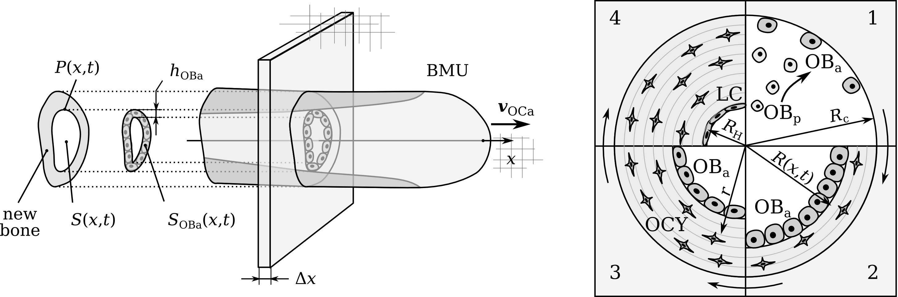
Figure 1: (a) The slice of bone of thickness $\Delta x$ at the fixed position $x$ reveals a transverse cross-section of the BMU (which itself progresses along the $x$ axis at speed $v_{\text{{OC}${}_{\text{a}}$}}$). The section exibits the ring-like cross-sectional area of newly-formed bone, the cross-sectional area of the cavity $\text{$S$}(x,t)$, the cross-sectional perimeter of the cavity $\text{$P$}(x,t)$, and the ring-like cross-sectional area containing active osteoblasts $\text{$S_{\text{{OB}${}_{\text{a}}$}}$}(x,t)$, of width $h_{\text{{OB}${}_{\text{a}}$}}$. (b) Four stages of the formation phase of the BMU seen in transverse cross-section at the fixed location $x$ in bone as the BMU progresses forward along $x$: 1. Onset of formation: differentiation of pre-osteoblasts (OB${}_{\text{p}}$) into active osteoblasts (OB${}_{\text{a}}$); cavity radius equal to the cement line radius $R_{\text{c}}$; 2. Early stage of formation, showing that some osteoblasts have become osteocytes (OCY) embedded in the bone matrix; cavity radius $\text{$R$}(x,t)$; 3. Mid stage of formation; $r$ denotes a radial coordinate; 4. End of formation: the active osteoblasts have become bone lining cells (LC) and the cavity radius is the Harversian canal radius $R_{\text{H}}$.

We consider a thin slice of bone exhibiting the refilling process in the closing cone of a BMU (Figure 1a). The slice corresponds to a local region of interest and is assumed to be (i) transverse to the BMU’s longitudinal axis ($x$); (ii) of small thickness $\Delta x$; and (iii) at a fixed position $x$ in bone (but the state of the BMU at various positions $x$ will be investigated).

As the BMU progresses forward along $x$, gradually moving away from the slice, the BMU cavity (Cv) seen in the slice refills with time due to the local production of osteoid by active osteoblasts (Figure 1b). The total volume of osteoid produced per unit time in the slice is $\text{$k_{\text{form}}$}(x,t)\Delta N_{\text{{OB}${}_{\text{a}}$}}(x,t)$, where $\text{$k_{\text{form}}$}(x,t)~{}[\micro^{3}/\text{day}]$ is the volume of osteoid secreted per osteoblast per unit time, and $\Delta N_{\text{{OB}${}_{\text{a}}$}}(x,t)$ is the number of active osteoblasts in the slice. The production of osteoid reduces the cross-sectional area of the BMU cavity $\text{$S$}(x,t)$ (Figure 1a) according to:

$$\tfrac{\partial}{\partial t}\text{$S$}(x,t)\,\Delta x=-\text{$k_{\text{form}}$}(x,t)\ \Delta N_{\text{{OB}${}_{\text{a}}$}}(x,t).$$ (3)

Dividing Eq. (3) by $\Delta x$, this can be expressed as:

$$\tfrac{\partial}{\partial t}\text{$S$}(x,t)=-\text{$k_{\text{form}}$}(x,t)\ \rho_{\text{{OB}${}_{\text{a}}$}}(x,t)\ \text{$P$}(x,t),$$ (4)

where

$$\rho_{\text{{OB}${}_{\text{a}}$}}(x,t)=\frac{\Delta N_{\text{{OB}${}_{\text{a}}$}}(x,t)}{\Delta x\,\text{$P$}(x,t)}$$ (5)

is the local surface density of active osteoblasts and $\text{$P$}(x,t)$ is the cross-sectional perimeter of the BMU cavity (Figure 1a). For a perfectly cylindrical cortical BMU of cavity radius $\text{$R$}(x,t)$, $\text{$P$}(x,t)=2\pi\text{$R$}(x,t)$, $\text{$S$}(x,t)=\pi\text{$R$}(x,t)^{2}$, and so $\tfrac{\partial}{\partial t}\text{$S$}=2\pi\text{$R$}\tfrac{\partial}{\partial t}\text{$R$}$. In this case, Eq. (4) specialises to Eq. (1):

$$\tfrac{\partial}{\partial t}\text{$R$}(x,t)=-\text{$k_{\text{form}}$}(x,t)\ \rho_{\text{{OB}${}_{\text{a}}$}}(x,t).$$ (6)

The refilling dynamics(4) and (6) are based on geometrical considerations only. These expressions do not depend on a specific model of osteoblast surface density $\rho_{\text{{OB}${}_{\text{a}}$}}$ or osteoid secretion rate $k_{\text{form}}$. In this paper, we will restrict to the refilling dynamics of cylindrical BMUs, Eq. (6).

2.2 Computational model for osteoblast distribution in the BMU

The mathematical model presented in this paper is based on our previous mathematical model of osteoclast and osteoblast development in a cortical BMU in one spatial dimension (the BMU longitudinal axis) [41]. Biochemical coupling between osteoclasts and osteoblasts and migration properties of these cells are implemented via the material balance equation expressed for each cell type and signalling molecule considered [41]. These equations integrate source and sink terms due to cell differentiation and cell apoptosis, receptor–ligand binding reactions, protein expression by cells, micro-environmental protein degradation, as well as transport terms due to cell migration and protein diffusion. The core assumptions of the model are summarised below with the network of biochemical regulation illustrated in Figure 2. Further details are presented in Appendix A, including all the governing equations and parameters of the model.

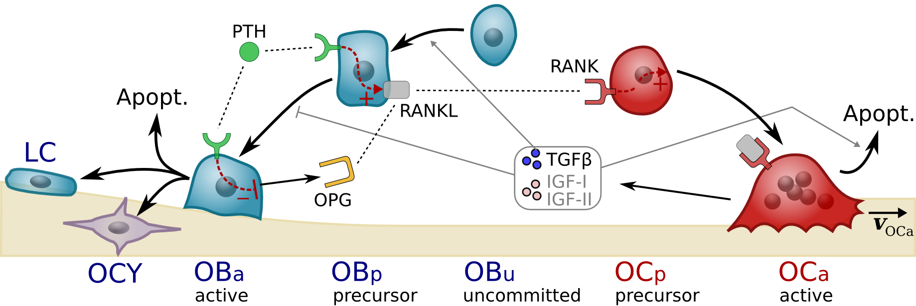
Figure 2: Biochemical regulation of osteoclast and osteoblast development in the BMU used in the model.

BMU cavity

The BMU cavity is assumed to be perfectly cylindrical (rotation-symmetric with respect to the $x$ axis). Only the refilling of the cavity is considered in this paper. The cavity radius $R(x,t)$ is assumed to decrease from an initial value equal to the cement line radius $R_{c}$ up to the Haversian canal radius $R_{H}$ (at most) due to matrix deposition by osteoblasts (Eq. (6)). The two parameters $R_{c}\approx 100~{}\micro$ and $R_{H}\approx 20~{}\micro$ correspond to human average values (see Table 3 in Appendix A). No cross-sectional variability is assumed for $R_{c}$ and $R_{H}$ in this paper. The model results will be compared with tetracycline data (Figure 4) that have been first normalised adequately to remove the influence of cross-sectional variability in cement line and Haversian canal radii [20], and that have been then rescaled to the values $R_{c}$ and $R_{H}$ assumed here.

Osteoclasts

Two stages of osteoclast development are modelled: pre-osteoclasts (OC${}_{\text{p}}$) and active osteoclasts (OC${}_{\text{a}}$) (Figure 2):

• OC${}_{\text{p}}$s are distributed around the tip of a blood vessel growing at a rate commensurate with the BMU progression ($20$–$40~{}\micro/\text{day}$) [1, 2, 44, 11], taken to be $30~{}\micro/\text{day}$;

• OC${}_{\text{p}}$s differentiate into OC${}_{\text{a}}$s at a rate $\mathcal{D}_{\text{{OC}${}_{\text{p}}$}}$ accelerated by activation of the receptor–activator of nuclear factor $\kappa$B (RANK) by the ligand RANKL [45, 46];

• OC${}_{\text{a}}$s undergo apoptosis at a rate $\mathcal{A}_{\text{{OC}${}_{\text{a}}$}}$ accelerated by transforming growth factor $\beta$ (TGF$\upbeta$) [45, 31];

• OC${}_{\text{a}}$s progress forward along the $x$ axis due to bone resorption, at a rate $v_{\text{{OC}${}_{\text{a}}$}}=30~{}\micro/\text{day}$ [1, 2, 11].

As a result, the material balance equation for the local volumetric density of active osteoclasts $\text{{OC}${}_{\text{a}}$}(x,t)~{}[^{-3}]$ is [41]:

$$\tfrac{\partial}{\partial t}\text{{OC}${}_{\text{a}}$}=\mathcal{D}_{\text{{OC}${}_{\text{p}}$}}(\text{{RANKL}})\,\text{{OC}${}_{\text{p}}$}-\mathcal{A}_{\text{{OC}${}_{\text{a}}$}}(\text{{TGF{$\upbeta$}}})\,\text{{OC}${}_{\text{a}}$}-\tfrac{\partial}{\partial x}(\text{{OC}${}_{\text{a}}$}\,v_{\text{{OC}${}_{\text{a}}$}}).$$ (7)

Osteoblasts

Three stages of osteoblast development are modelled: uncommitted osteoblast progenitors (such as mesenchymal stem cells) (OB${}_{\text{u}}$), pre-osteoblasts (OB${}_{\text{p}}$) and active osteoblasts (OB${}_{\text{a}}$). Osteoblasts may also become osteocytes (OCY) or bone lining cells (LC) (Figure 2):

• OB${}_{\text{u}}$s are distributed around the tip of the blood vessel growing along $x$ at $30~{}\micro/\text{day}$, similarly to OC${}_{\text{p}}$s [1, 47, 2, 44];

• OB${}_{\text{u}}$s differentiate into OB${}_{\text{p}}$s at a rate $\mathcal{D}_{\text{{OB}${}_{\text{u}}$}}$ accelerated by TGF$\upbeta$ [2, 5, 48, 49];

• OB${}_{\text{p}}$s differentiate into OB${}_{\text{a}}$s at a rate $\mathcal{D}_{\text{{OB}${}_{\text{p}}$}}$ inhibited by TGF$\upbeta$ [31, 41];

• OB${}_{\text{p}}$s and OB${}_{\text{a}}$s are stationary with respect to bone [2, 1, 41, 50, 51].

The following features of osteoblast development are added in the present work compared to Ref. [41] (see Appendix A for more details):

• Secretory activity. The secretory activity of OB${}_{\text{a}}$s depends on the current cavity radius:

  $$\text{$k_{\text{form}}$}(x,t)=\widetilde{k}_{\text{form}}\big{(}\text{$R$}(x,t)\big{)}\quad[\micro^{3}/\text{day}]$$ (8)

  The function $\widetilde{k}_{\text{form}}$ elucidating this dependence is extrapolated from measurements from [21]. The activity of osteoblasts is thereby assumed to vary continuously (e.g., no work–rest cycles) [11, 1, 52];

• Osteoblast-to-osteocyte transition. OB${}_{\text{a}}$s transition to OCYs at a rate $\sigma_{\text{{OCY}}}^{\text{prod.}}$ that depends on the density of OB${}_{\text{a}}$s and on $R$ [22, 53, 36], such that a uniform density of OCYs of $$20\,000$/^{3}$ is produced [11];

• Osteoblast-to-bone lining cell transition. OB${}_{\text{a}}$s transition to LC when $R$ reaches a target Haversian canal radius $R_{\text{H}}$. This is modelled by a sudden, but continuous drop in OB${}_{\text{a}}$s’ secretory activity $\widetilde{k}_{\text{form}}(\text{$R$})$ near $R_{\text{H}}$ [1] (see Figure 6 in Appendix A);

• Osteoblast apoptosis. OB${}_{\text{a}}$s undergo apoptosis at a constant rate $A_{\text{{OB}${}_{\text{a}}$}}$ calibrated so as to eliminate osteoblasts ‘in surplus’ [1, 2];

• Geometric influence of BMU cavity shrinkage. The shrinking BMU cavity confines OB${}_{\text{a}}$s into a smaller space, which increases the density of OB${}_{\text{a}}$s at a rate $G$ that depends on $R$ [36, 54].

The total change in the density of OB${}_{\text{a}}$s is a superposition of all of the influences listed above, which may compensate each other. In particular, the density of OB${}_{\text{a}}$s may still decrease during BMU cavity shrinkage if there is a concurrent decrease in the number of OB${}_{\text{a}}$s in the cavity. As a result of the above assumptions, the material balance equations for the local volumetric densities of pre-osteoblasts $\text{{OB}${}_{\text{p}}$}(x,t)$ and active osteoblasts $\text{{OB}${}_{\text{a}}$}(x,t)$ are:

$$\tfrac{\partial}{\partial t}\text{{OB}${}_{\text{p}}$}=\mathcal{D}_{\text{{OB}${}_{\text{u}}$}}(\text{{TGF{$\upbeta$}}})\,\text{{OB}${}_{\text{u}}$}-\mathcal{D}_{\text{{OB}${}_{\text{p}}$}}(\text{{TGF{$\upbeta$}}})\,\text{{OB}${}_{\text{p}}$}$$ (9)

$$\tfrac{\partial}{\partial t}\text{{OB}${}_{\text{a}}$}=\mathcal{D}_{\text{{OB}${}_{\text{p}}$}}(\text{{TGF{$\upbeta$}}})\,\text{{OB}${}_{\text{p}}$}-A_{\text{{OB}${}_{\text{a}}$}}\,\text{{OB}${}_{\text{a}}$}+G\,\text{{OB}${}_{\text{a}}$}-\sigma_{\text{{OCY}}}^{\text{prod.}}$$ (10)

The last three terms of Eq. (10) replace the constant elimination rate of OB${}_{\text{a}}$s used in Ref. [41], which was previously modelling all the depletion pathways of the pool of active osteoblasts (i.e., osteoblast-to-osteocyte, osteoblast-to-bone lining cell, and apoptosis). The precise form of these new terms (in particular, their dependence on the cavity radius $\text{$R$}(x,t)$) is presented in Appendix A.

Signalling molecules and binding reactions

The biochemical coupling between osteoclasts and osteoblasts is mediated in the model by RANKL and TGF$\upbeta$, as in Refs [31, 41] (TGF$\upbeta$ may also represent other regulatory factors stored in the bone matrix, such as insulin-like growth factors (IGF), see Figure 2). RANKL is influenced by osteoprotegerin (OPG) and parathyroid hormone (PTH). All of RANKL, OPG and TGF$\upbeta$ are driven by cellular actions (Figure 2):

• RANKL is expressed on the membrane of OB${}_{\text{p}}$s; OPG is expressed by OB${}_{\text{a}}$s; RANK is expressed on OC${}_{\text{p}}$s [55, 56, 41];

• RANKL binds both RANK and the decoy receptor OPG competitively (RANK signalling on OC${}_{\text{p}}$ is thereby diminished in presence of OPG) [45, 46];

• PTH promotes the expression of RANKL and inhibits the expression of OPG [57]. In this work, a constant level of systemic PTH is assumed, uniformly distributed along the BMU [41].

• TGF$\upbeta$ is stored in the bone matrix at a constant concentration $n^{\text{bone}}_{\text{{TGF{$\upbeta$}}}}$; it is released in the micro-environment in proportion to bone resorption by OC${}_{\text{a}}$s [45, 48, 49];

• All of the signalling molecules RANKL, OPG, and TGF$\upbeta$ undergo micro-environmental degradation at a constant rate. A constant number of RANK per OC${}_{\text{p}}$ is assumed.

Binding reactions between receptors and ligands are considered through mass action kinetics with reaction rates proportional to population sizes. The acceleration or inhibition of a cell behaviour by a ligand, such as differentiation rate, apoptosis rate, and protein production rate, is assumed to occur in proportion to the receptor occupancy on the cell (see Appendix A and Ref. [41] for further details).

Surface density and volumetric density of active osteoblasts

Biochemical processes of cell development are best described in terms of volumetric concentrations of signalling molecules and volumetric density of cells. (To align with common practice, we use the terminology ‘concentration’ for signalling molecules and ‘density’ for cells, even though both terminologies refer to the same units, i.e., number per unit volume.) Indeed, biochemical reaction rates depend on the probability of encounter of the interacting biochemical compounds. This probability depends in turn on how closely packed the compounds are, and so, on their local concentration or density (i.e., their number per unit volume) [58].

The material-balance equations (7)–(10), which involve biochemical reactions, are therefore written in terms of volumetric densities. However, the refilling dynamics described by Eq.(6) involves the surface density $\rho_{\text{{OB}${}_{\text{a}}$}}$ of active osteoblasts. To relate the volumetric density OB${}_{\text{a}}$ to the surface density $\rho_{\text{{OB}${}_{\text{a}}$}}$, we use the fact that active osteoblasts in a BMU form a single layer of cells against the cavity walls [21], of thickness $h_{\text{{OB}${}_{\text{a}}$}}$ (the height of an active osteoblast). In the cross section, active osteoblasts are thus confined to an annulus of cross-sectional area $S_{\text{{OB}${}_{\text{a}}$}}$ (Figure 1a). Within this annulus, active osteoblasts are distributed fairly uniformly, and so $S_{\text{{OB}${}_{\text{a}}$}}$ constitutes an appropriate representative surface element to define the volumetric density of active osteoblasts [58, Chap. XIV], i.e.:

$$\text{{OB}${}_{\text{a}}$}(x,t)=\frac{\Delta N_{\text{{OB}${}_{\text{a}}$}}(x,t)}{\Delta x\ \text{$S_{\text{{OB}${}_{\text{a}}$}}$}(x,t)}=\rho_{\text{{OB}${}_{\text{a}}$}}(x,t)\frac{\text{$P$}(x,t)}{\text{$S_{\text{{OB}${}_{\text{a}}$}}$}(x,t)},$$ (11)

where Eq. (5) has been used for the second equality. In a cylindrical BMU, $\text{$P$}(x,t)=2\pi\text{$R$}(x,t)$ and

$$\text{$S_{\text{{OB}${}_{\text{a}}$}}$}(x,t)=\pi\big{[}\text{$R$}(x,t)^{2}-(\text{$R$}(x,t)-\text{$h_{\text{{OB}${}_{\text{a}}$}}$})^{2}\big{]}.$$ (12)

The relation (11) between osteoblast surface density and volumetric density becomes:

$$\rho_{\text{{OB}${}_{\text{a}}$}}(x,t)=\text{{OB}${}_{\text{a}}$}(x,t)\ \text{$h_{\text{{OB}${}_{\text{a}}$}}$}\left(1-\frac{\text{$h_{\text{{OB}${}_{\text{a}}$}}$}}{2\text{$R$}(x,t)}\right).$$ (13)

Substituting Eq. (13) into Eq. (6) gives:

$$\tfrac{\partial}{\partial t}\text{$R$}(x,\!t)=-\text{$k_{\text{form}}$}(x,\!t)\text{{OB}${}_{\text{a}}$}(x,\!t)\text{$h_{\text{{OB}${}_{\text{a}}$}}$}\!\left(\!\!1\!-\!\frac{\text{$h_{\text{{OB}${}_{\text{a}}$}}$}}{2\text{$R$}(x,\!t)}\!\!\right)\!.$$ (14)

We note that in the above relationship, the geometric factor $\big{(}1-\frac{\text{$h_{\text{{OB}${}_{\text{a}}$}}$}}{2\text{$R$}(x,t)}\big{)}$ accounts for the nonzero curvature $1/\text{$R$}$ of the cavity (a flat surface has zero curvature, corresponding to the limiting case $1/\text{$R$}\to 0$). However, both $k_{\text{form}}$ and OB${}_{\text{a}}$ may still depend on $R$.

Calibration of the cell populations and validation of the model

Quantitative data on the distribution of cells and their total number in cortical BMUs are relatively sparse [47, 43, 21, 2]. Some of the data useful to calibrate and validate our model are derived from animal models, such as cell surface densities and osteoid secretion rates at different BMU cavity radii (dogs) [21], total cell numbers (dogs) [43], and tetracycline double labelling radii (sheep) [20]. Some of these data were rescaled to (pseudo-)human values according to known (or suspected) cross-species differences [59] (Appendix A). We calibrated our model such that the numerical cell distribution profiles are in reasonable agreement with the following:

• The total number of precursor cells ($N_{\text{{OB}${}_{\text{u}}$}},N_{\text{{OC}${}_{\text{p}}$}}$) in steady state is about 20;

• The total number of active osteoclast nuclei ($N_{\text{{OC}${}_{\text{a}}$}}$) in steady state is about 100 [43]. (Here and in Ref. [41], OC${}_{\text{a}}$s represent mononucleated entities incorporated in a multinucleated active osteoclast. Multinucleated active osteoclasts are composed of about 10 nuclei [43];)

• The surface density of active osteoblasts ($\rho_{\text{{OB}${}_{\text{a}}$}}$) in steady state coincides with data reported by Marotti et al. [21] at three different cavity radii (appropriately rescaled), whilst the total number of active osteoblasts ($N_{\text{{OB}${}_{\text{a}}$}}$) in steady state is in the range $2000$–$6000$ [43, 11, 36] (see also Discussion, Section 4).

To calibrate the model against the number of active osteoclast nuclei and precursor cells in the steady-state BMU, the cell densities $\text{{OC}${}_{\text{a}}$}(x,t)$, $\text{{OC}${}_{\text{p}}$}(x,t)$ and $\text{{OB}${}_{\text{u}}$}(x,t)$ were integrated over the BMU cavity volume at $t=150~{}\text{days}$. Appropriate changes in model parameter values were determined to enable these cell numbers to match the values mentioned above (Appendix A, Eqs (22)).

To calibrate the model against the surface densities of active osteoblasts at three different cavity radii (Table 2) and against the total number of active osteoblasts, we modified (i) the rate of osteoblast apoptosis $A_{\text{{OB}${}_{\text{a}}$}}$; (ii) the model parameters related to the scaling factor $\alpha_{\text{{OB}${}_{\text{a}}$}}$ (Appendix A); and (iii) the (canine-to-human) scaling factor $\alpha_{\text{$k_{\text{form}}$}}$ (Appendix A). The apoptosis rate $A_{\text{{OB}${}_{\text{a}}$}}$ influences the spatial rate of decrease of the osteoblast distribution at the back of the BMU [41]. The factor $\alpha_{\text{{OB}${}_{\text{a}}$}}$ scales the value of the density at each location along the BMU uniformly. The scaling factor $\alpha_{\text{$k_{\text{form}}$}}$ enables to modify the total number of active osteoblasts in the steady state BMU (e.g., increasing $\alpha_{\text{$k_{\text{form}}$}}$ reduces $N_{\text{{OB}${}_{\text{a}}$}}$). The total number of pre-osteoblasts was obtained by integrating $\text{{OB}${}_{\text{p}}$}(x,t)$ over the cavity volume and the total number of active osteoblasts was obtained by integrating the surface density $\rho_{\text{{OB}${}_{\text{a}}$}}(x,t)$ over the cavity–bone surface in the steady state BMU (at $t=150~{}\text{days}$).

The calibrated model was validated against three independent sets of experimental data: (i) the density of bone lining cells reached at the end of the formation phase; (ii) the length of the closing cone of the BMU; (iii) tetracycling double labelling data (see Sections 3 and 4).

Governing equations and numerical simulations

Equations (7)–(10) and Eq. (14) govern the dynamics of the cell populations in the BMU and of the BMU cavity refilling. These equations are interdependent and involve binding reactions for the concentrations of RANKL, OPG, and TGF$\upbeta$. TGF$\upbeta$ has a production rate that depends on osteoclast resorption, but the dynamics of the signalling molecules RANKL and OPG is fast compared to the characteristic times of cell behaviours [41]. The balance equations of RANKL and OPG can be taken in a quasi-steady state, enabling the concentration of these signalling molecules to become algebraic expressions of the variables $\text{{OB}${}_{\text{p}}$},\text{{OB}${}_{\text{a}}$},\text{{OC}${}_{\text{a}}$}$, and TGF$\upbeta$ [41].

The equations governing the evolution of the whole system are presented in Appendix A, see Eqs (23)–(26). These equations together with Eq. (14) form a coupled system of five partial differential equations (PDEs). These PDEs were solved numerically to evolve the system for 150 days from an initial condition with a small, localised population of active osteoclast nuclei (OC${}_{\text{a}}$s) and given distributions of OB${}_{\text{u}}$s and OC${}_{\text{p}}$s concentrated around the (growing) tip of the blood vessel of the BMU, as in Ref. [41]. The initial cavity radius was set to the cement line radius $R_{\text{c}}$ as only the refilling of the cavity is considered in this paper. The point of origin of the BMU (i.e., the center of the initial distribution of active osteoclasts and precursor cells) was set at $x_{0}=-4.85~{}$. The PDEs were solved in a co-moving frame attached to the BMU with the following boundary conditions: the density of pre-osteoblasts and active osteoblasts was set to zero at the (moving) front of the BMU; the density of active osteoclasts and the concentration of TGF$\upbeta$ were set to zero at the back of the BMU. The numerical algorithm used was that of the ‘method of lines’ of Mathematica’s PDE solver ‘NDSolve’ with a spatial discretisation of at least 2000 points, ensuring absolute and relative tolerances of $10^{-4}$ [60].

3 Results

Evolution of the cell distribution profiles: BMU initiation and quasi-steady state

The distribution of cells along the longitudinal $x$ axis evolves from the initial condition into a stable multicellular travelling-wave-like structure (Figure 3a–c). After an initiation phase during which the shapes of the cell distribution profiles develop and stabilise, this multicellular structure progresses forward through bone without changing shape (‘quasi-steady’ state), with osteoclasts towards the front and osteoblasts towards the back, as in a BMU (Figure 3c).

Figure 3: (a)–(c) The profiles of cell densities along the BMU’s length (top of each panel) and the corresponding shape of the closing cone (bottom of each panel) are shown at time (a) $t=0\ \text{days}$ (initial condition), (b) $t=75\ \text{days}$, and (c) $t=150\ \text{days}$. To ensure that all cell densities are visible, OB${}_{\text{u}}$, OC${}_{\text{p}}$, and OC${}_{\text{a}}$ were multiplied by a factor 20. The active osteoblast surface density $\rho_{\text{{OB}${}_{\text{a}}$}}$ and bone lining cell surface density $\rho_{\text{{LC}}}$ are also shown (dot-dashed lines). In (b), individual osteoid secretion rate $k_{\text{form}}$ has not yet dropped enough for OB${}_{\text{a}}$ to differentiate into LC. In (c), an $\text{{OB}${}_{\text{a}}$}\to\text{{LC}}$ transition takes place as indicated by the arrow. The arrow starts and ends where $k_{\text{form}}$ is 90% and 10% of the drop near $R_{\text{H}}$ in Figure 6 (see also panel (d)). The crosses in (c) correspond to the experimental data of osteoblast surface density from [21] listed in Table 2, scaled to human values. (d) Profile of osteoid secretion rate $\text{$k_{\text{form}}$}(x,t)$ by active osteoblasts at $t=150\ \text{days}$. The grey lines indicate where $k_{\text{form}}$ is 90% and 10% of the drop near $R_{\text{H}}$ in Figure 6 ($\text{{OB}${}_{\text{a}}$}\to\text{{LC}}$ transition).

Each cell type reaches a stable spatial distribution at a different rate. The population of active osteoclasts quickly increases from almost zero to its quasi-steady state within around $10~{}\text{days}$. In contrast, the population of active osteoblasts takes about $130~{}\text{days}$ until its spatial distribution reaches a stable shape. However, the shape of the front of the OB${}_{\text{a}}$ distribution profile (i.e., the part ahead of the maximum) takes less time to stabilise, approximately $50~{}\text{days}$. The comparison of Figures 3b and 3c shows that the front of the OB${}_{\text{a}}$ distribution profile (including a part extending beyond the maximum) has reached a stable shape by $t=75~{}\text{days}$. In fact, the time required for the front of the OB${}_{\text{a}}$ distribution profile to reach a steady shape ($50~{}\text{days}$) corresponds to the time required to increase the population of active osteoblasts from zero to its maximum value when the BMU is initiating. All the bone traversed by the BMU at times $t\gtrsim 50~{}\text{days}$, i.e. all the bone located at $x\gtrsim-4.1~{}$, experiences the full extent of the population of both active osteoclasts and active osteoblasts ($-4.1~{}$ corresponds to the position of the maximum of the active osteoblast population at $t=50~{}\text{days}$). The temporal pattern of osteoclast and osteoblast development seen at these fixed locations in bone whilst traversed by the BMU is no longer developing as during the initiation stage of the BMU. At these locations, the BMU is seen in a quasi-steady state, and the time required to increase the population of active osteoblasts to its maximum value is reduced to about $26~{}\text{days}$ (see below).

BMU cavity shape (closing cone)

The BMU cavity shown at the bottom of each graph in Figure 3a–c progressively refills as soon as active osteoblasts are generated. During the initiation stage of the BMU, the shape of the closing cone varies. When the BMU reaches its quasi-steady state, the closing cone is fully formed and progresses forward without changing shape, in association with the quasi-steady population of active osteoblasts. Matrix apposition rate is strongly reduced when the cavity radius reaches values close to the ‘target’ Haversian canal radius $\text{$R_{\text{H}}$}=20\ \micro$. The variation of osteoid secretion rate per osteoblast along the BMU, $\text{$k_{\text{form}}$}(x,t)$, is shown at $t=150\ \text{days}$ in Figure 3d. The locations at which $k_{\text{form}}$ is 90% and 10% of the magnitude of the drop near $\text{$R$}=\text{$R_{\text{H}}$}$ in Figure 6 (see Appendix A) are also shown (gray lines). These locations indicate the transition of active osteoblasts (OB${}_{\text{a}}$s) into bone lining cells (LC) and correspond to the start and end of the $\text{{OB}${}_{\text{a}}$}\to\text{{LC}}$ transition arrow in Figure 3c. This transition represents the end of the (active) BMU closing cone, and the start of the (quiescent) newly-formed osteon.

Length of the closing cone

Considering the start of the closing cone in Figure 3c to be around $x\approx-0.5~{}$ and the end of the closing cone to correspond to the intersection of the active osteoblast surface density and bone lining cell density at around $x\approx-3~{}$, the total length of the closing cone of the simulated BMU is about $2.5~{}$.

Osteoblast density and total cell numbers in the BMU

In the steady-state BMU shown in Figure 3c, the population of active osteoblasts (OB${}_{\text{a}}$, blue) rises sharply at the start of the refilling process, i.e. between $x\approx-0.35~{}$ and $x\approx-1.12~{}$, the latter being the position of the maximum density. This spatial interval corresponds to a time interval of about $26~{}\text{days}$ $\big{(}\!\!\equiv\!\!\tfrac{(-1.12+0.35)~{}}{30~{}\micro/\text{day}}\big{)}$. The peak population of active osteoblasts is reached near the disappearance of the population of pre-osteoblasts (OB${}_{\text{p}}$, cyan). Past this point, the distribution of active osteoblasts exhibits a slow, pseudo-linear decrease (from right to left) up to the point where active osteoblasts transition to bone lining cells ($\text{{LC}}\to\text{{OB}${}_{\text{a}}$}$ arrow).

The dot-dashed blue line in Figure 3c represents the surface density of active osteoblast $\rho_{\text{{OB}${}_{\text{a}}$}}$ and the constant surface density of bone lining cells $\rho_{\text{{LC}}}=2300/^{2}$ [11]. Surface densities $\rho_{\text{{OB}${}_{\text{a}}$}}<2300/^{2}$ are shaded as they do not correspond to real active osteoblasts: at these locations, osteoblasts are assumed to have become bone lining cells of constant density no longer secreting osteoid and no longer undergoing apoptosis. The transition from active osteoblasts to bone lining cells (driven by the current value of the BMU cavity radius) occurs precisely when the surface density of active osteoblasts reaches values around $2300/^{3}$.

With the model parameters listed in Table 3 in Appendix A, the total number of each cell type found in the simulated BMU is (up to rounding approximations):

$$N_{\text{{OC}${}_{\text{a}}$}}\approx 100,\quad N_{\text{{OC}${}_{\text{p}}$}}\approx 20,\quad N_{\text{{OB}${}_{\text{u}}$}}\approx 20$$ (15)

$$N_{\text{{OB}${}_{\text{p}}$}}\approx$11\,100$,\qquad N_{\text{{OB}${}_{\text{a}}$}}\approx$5200$.$$ (16)

The experimental data on osteoblast surface density at different cavity radii, scaled to correspond to human average BMUs (crosses in Figure 3c), are matched by the calibrated numerical surface density $\rho_{\text{{OB}${}_{\text{a}}$}}$.

Figure 4: Matrix apposition rate versus BMU cavity radius obtained from our model (lines) and from tetracycline experiments (dots). The exact matrix apposition rate $\big{|}\tfrac{\partial}{\partial t}\text{$R$}(x,t)\big{|}$ versus $\text{$R$}_{1}\equiv\text{$R$}(x,t)$ is shown at position $x=-3.5~{}$ in bone (solid grey line). The approximate matrix apposition rates $\big{|}\tfrac{\text{$R$}_{2}-\text{$R$}_{1}}{\Delta t}\big{|}\equiv\big{|}\tfrac{\text{$R$}(x,t+\Delta t)-\text{$R$}(x,t)}{\Delta t}\big{|}$ versus $\text{$R$}_{1}\equiv\text{$R$}(x,t)$ are shown at $x=-2.5~{}$, $-3.5~{}$, $-4.5~{}$, $-4.65$, and $-4.7~{}$ for a fixed interval $\Delta t=10~{}\text{days}$. Data points are taken from Ref. [20, Fig. 2] and have been appropriately rescaled to human average BMU sizes (see text).

[vecscale=0.85]fig-R2-vs-R1

Figure 5: Parametric plots of cavity radius pairs $(\text{$R$}_{1},\text{$R$}_{2})$ with $\text{$R$}_{1}=\text{$R$}(x,t)$ and $\text{$R$}_{2}=\text{$R$}(x,t+\Delta t)$ obtained from our model at a fixed location in bone ($x=-4~{}$) when $t$ evolves from $0$ to $150~{}\text{days}$. The figure shows the effect of choosing different time intervals $\Delta t=$ 10 days, 12 days, and 15 days (corresponding to typical time intervals between tetracyline injections). The calculated curves intersect with the diagonal at the onset of formation and at completion of formation.

Tetracycline double labelling data

In Figure 4 we plot the ‘exact’, instantaneous matrix apposition rate $|\tfrac{\partial}{\partial t}\text{$R$}(x,t)|$ versus $\text{$R$}(x,t)$ at $x=-3.5~{}$ (solid grey line) and the approximate, average matrix apposition rates (MAR) $\big{|}\tfrac{\text{$R$}(x,t+\Delta t)-\text{$R$}(x,t)}{\Delta t}\big{|}$ versus $\text{$R$}(x,t)$ obtained in our simulations during refilling when $t$ evolves from $0$ to $150~{}\text{days}$. The effect of sampling the radii at various positions $x$ in bone is shown (solid and interrupted black lines), whilst the time interval $\Delta t=10~{}\text{days}$ (corresponding to the interval between tetracycline injections in Ref. [20]) is kept fixed. These results are compared to experimental data from Ref. [20]. This data was collected in sheep and plotted in Ref. [20, Fig. 2] as MAR versus “percent unfilled”, i.e., the percent of bone thickness remaining to deposit so as to reach the sheep Haversian canal radius. In Figure 4, we rescaled this “percent unfilled” data to human-sized BMU cavity radii, such that 100% unfilled corresponds to the cement line radius $\text{$R_{\text{c}}$}=100~{}\micro$ and 0% unfilled corresponds to the Haversian canal radius $\text{$R_{\text{H}}$}=20~{}\micro$ (see Eq. (20) in Appendix A).

Tetracycline double labelling data is sometimes presented as a plot of the data pairs $(\text{$R$}_{1},\text{$R$}_{2})$ [16, 20, 19]. In Figure 5 we plot the trajectory of the radii pairs $\big{(}\text{$R$}(x,t),\text{$R$}(x,t+\Delta t)\big{)}$ obtained during refilling for various time intervals $\Delta t$ when $t$ evolves from $0$ to $150~{}\text{days}$ at the fixed location $x=-3.5~{}$.

4 Discussion

Cell distribution profiles within the BMU

The emergence and progression of structured cell distribution profiles models the initiation and quasi-steady phases of a cortical BMU. A key role is played by the biochemical coupling between the bone cells and by the cell migration properties to explain the emergence and stability of the BMU [41]. The cells present initially at $t=0$ generate a biochemical positive feedback loop, captured in the governing equations: the OC${}_{\text{a}}$s free TGF$\upbeta$ from the bone matrix into the microenvironment, which promotes the differentiation of OB${}_{\text{u}}$s into OB${}_{\text{p}}$s. The ligand RANKL expressed on OB${}_{\text{p}}$s promotes in turn the differentiation of OC${}_{\text{p}}$s into OC${}_{\text{a}}$s, thus enabling the process to be sustained. Further towards the back of the BMU, the concentration of TGF$\upbeta$ drops [41]. This facilitates the differentiation of OB${}_{\text{p}}$s into OB${}_{\text{a}}$s [2, 3]. At this point, bone formation starts and the cavity refills.

The shape of the cell distribution profile of active osteoblasts (OB${}_{\text{a}}$) is appreciably modified compared to Ref. [41, Fig. 2] due to the additional influences on osteoblast development considered. The increase in the density of OB${}_{\text{a}}$s is sharper at the start of formation whilst its decrease towards the back of the BMU is slower, exhibiting a pseudo-linear behaviour that contrasts with the exponential-like decrease obtained in [41]. This slower decrease is attributable to the tendency of cavity shrinkage to concentrate the density of active osteoblasts, which partly compensates the depletion pathways of the pool of active osteoblasts [54]. This enabled us to calibrate the model so as to match Marotti et al.’s data on the surface density $\rho_{\text{{OB}${}_{\text{a}}$}}$ reasonably well.

The strong influence of cavity shrinkage on $\rho_{\text{{OB}${}_{\text{a}}$}}$ can be guessed by the fact that during refilling, the surface area of the BMU cavity walls shrinks to about 20% of its initial extent (ratio $\text{$R_{\text{H}}$}/\text{$R_{\text{c}}$}$). If the number of osteoblasts was conserved during refilling, their density would increase five-fold as they would be packed onto a much smaller surface. Osteoblast density still decreases due to their continuous elimination from the active pool, but at rate slowed down by the shrinking of the cavity.

Model robustness

The biochemical positive feedback loop between osteoblasts and osteoclasts is controlled (i) by elimination of the cell populations; (ii) by the negative feedback of TGF$\upbeta$ on the population of osteoclasts (see Figure 2); and (iii) by the fact that ligand activations saturate when all the receptors on the cell membranes are occupied. As a consequence, the qualitative behaviour of the model is generally very robust, unless drastic changes in the model structure are made (such as swapping the osteoblast cell types expressing RANKL and OPG, or changing the cell transport properties, see [41]). The inclusion of geometrical feedbacks on the osteoblast lineage (through secretory activity and osteocyte generation) can lead in some cases to more pronounced, but still continous, changes in the density of active osteoblasts. These changes are due to the sudden drop in secretory activity when $R\approx R_{H}$, which is accompanied by a sudden drop in the rate of osteoblast-to-osteocyte transition (since refilling is terminating). This can lead to a temporary increase in the density of active osteoblasts when their density is high (higher than the experimental data points of [21]). At normal densities, this phenomenon is manifested by a slight “bulge” in the density distribution near the osteoblast-to-osteocyte transition (Figure 3c).

BMU initiation and quasi-steady state

The life history of a BMU is usually divided into three separate stages: initiation (resorption alone, early life), progression (resorption and formation, mid life), and termination (formation alone, late life) [11]. From the dynamics of cell development observed in our model, these stages can be decomposed further into several levels of quasi-steady states until the progression stage is fully developed. Indeed, whilst the population of certain cell types may have reached a quasi-steady state within the BMU, the population of other cell types may still be developing. Due to the longer lifespan of osteoblasts compared to osteoclasts, we observe that osteoclast densities reach a steady state earlier in the BMU’s life than osteoblast densities. The sequence of cell types reaching a steady-state spatial distribution within the BMU is: (1) precursor cells (OB${}_{\text{u}}$, OC${}_{\text{p}}$) (this is assumed to occur instantly [41]); (2) active osteoclasts (OC${}_{\text{a}}$); (3) pre-osteoblasts (OB${}_{\text{p}}$); (4) active osteoblasts (OB${}_{\text{a}}$). The appearance of the first active osteoblasts in the BMU (which denotes the transition from the initiation to the progression stage according to the usual picture) occurs between stages (1) and (2). In Figure 3b (at $t=75~{}\text{days}$), the density of active osteoclasts (OC${}_{\text{a}}$) and of pre-osteoblasts (OB${}_{\text{p}}$) have already reached a quasi-steady state distribution, but not the density of OB${}_{\text{a}}$s near the back of the BMU. This state is situated between the stages (3) and (4) above, and corresponds to an early (still developing) progression stage.

According to this picture of cell and BMU development, a significant portion of the BMU’s lifespan of 6–12 months [2] could be spent in a developing (nonsteady) stage. The stabilisation of the spatial distribution profiles of cells occurs only once the BMU has travelled sufficiently far away from its point of origin ($\approx 130~{}\text{days}$). The temporal pattern of cells experienced at a single location in bone stabilises quicker (50 days). Unfortunately, this temporal pattern is not recorded in bone, unlike the spatial distribution of cells. The often depicted correspondence between temporal pattern at a fixed location and spatial distribution at a single time (see, e.g., [2, Figs 1–2]) occurs only once the BMU has fully developed stable spatial distributions of all its cell types. This could have important consequences for BMU-related properties of bone remodelling that are determined experimentally assuming steady-state BMUs, such as resorption and formation periods and activation frequencies [1, 11].

Osteoblast-to-osteocyte transition

The generation of osteocytes occurs by embedment of active osteoblasts into the bone matrix [22, 53]. This complex process is believed to involve a regulation of osteoblast secretory activity by the osteocytes themselves (e.g., via sclerostin). In the model, such a regulation is not accounted for, but the rate at which the osteoblast-to-osteocyte transition needs to occur so as to reproduce a given distribution of osteocytes is calculated (see Eq. (A)). Since both matrix apposition rate and BMU cavity radius decrease as refilling proceeds, the rate of the osteoblast-to-osteocyte transition (A) also decreases. A regulation by osteocytes combined with changes in the local curvature could explain this decrease [27]. However further studies are required to investigate the effect of potentially important factors, such as the mineralisation of the newly deposited matrix.

Osteoblast-to-bone lining cell transition

What regulates the transition from osteoblasts to quiescent bone lining cells at the back of a BMU remains poorly understood. In the model, this transition is driven by the current BMU cavity radius (via $k_{\text{form}}$ in Eq. (8)). A validation of our model of osteoblast development and of its calibration is provided by the fact that this transition occurs precisely where $\rho_{\text{{OB}${}_{\text{a}}$}}$ reaches observed values of bone lining cells surface densities ($\rho_{\text{{LC}}}\approx$2300$/^{2}$ [11]). This is indicated in Figure 3c by the fact that the $\rho_{\text{{OB}${}_{\text{a}}$}}$ curve intersects the $\text{{OB}${}_{\text{a}}$}\to\text{{LC}}$ transition arrow. When the distribution of active osteoblasts did not match the experimental points of [21] in Figure 3 due to poorly-calibrated model parameters, the following situations were encountered. For higher osteoblast densities, the cavity was refilled earlier, leading to lengths of the closing cone shorter than reported values, and to an osteoblast-to-bone lining cell transition occurring at surface densities higher than $$2300$/^{2}$. For lower osteoblast densities, the BMU cavity was either (i) refilled later, leading to lengths of the closing cone larger than reported value and to an osteoblast-to-bone lining cell transition occurring at surface densities smaller than $$2300$/^{2}$; or (ii) permanently under-refilled (i.e., not refilled up to the ‘target’ Haversian canal radius $R_{H}$) due the population of osteoblasts becoming extinct before they could reduce their secretory activity and become lining cells.

Osteoblast apoptosis

Osteoblast apoptosis in a BMU is believed to serve to eliminate ‘surplus’ osteoblasts, i.e., osteoblasts that are neither forming bone, nor becoming osteocytes, nor becoming bone lining cells [2]. The rate of osteoblast apoptosis, as a regulatory mechanism of osteoblast number in the closing cone, is thus likely to depend on the phase of the refilling process in the BMU. As the cavity shrinks, the number of osteocytes to be generated per unit time decreases and osteoblasts are confined into a smaller volume, resulting in an increase in surplus osteoblasts. The rate of osteoblast apoptosis $A_{\text{{OB}${}_{\text{a}}$}}\text{{OB}${}_{\text{a}}$}$ assumed in our model, which is proportional to the population size, enabled us to obtain a profile of active osteoblast surface density that accurately matched the experimental measurements of Marotti et al. [21] and the bone lining cell density. It is possible that comparison with more extensive data in the future may require $A_{\text{{OB}${}_{\text{a}}$}}$ to be dependent on the refilling stage (e.g., via $R$).

Number of osteoblasts within the BMU

Precise estimates of the total number of active osteoblasts in a BMU $N_{\text{{OB}${}_{\text{a}}$}}$ are difficult to find in the literature. Numbers of about $3000$ per millimetre of BMU length [36], in the range of $2000$–$4000$ [43], and up to $6750$ [11, Table 6] are reported. This variation may reflect cross-sectional variability, cross-species variability, and/or measurements performed on BMUs at different stages of their lifetime, and so having different closing cone lengths. Estimates of the local surface density of active osteoblasts $\rho_{\text{{OB}${}_{\text{a}}$}}$ are likely to be more reliable as they are based on local measurements and do not depend on the closing cone length.

A reasonable lower bound estimate of $N_{\text{{OB}${}_{\text{a}}$}}$ may be found by assuming a conical shape of the closing cone between $R_{\text{H}}$ and $R_{\text{c}}$, and a lower-bound surface density of 2300/² (surface density of bone lining cells [11]). With a closing cone length $L_{\text{form}}\approx 2.5~{}$ [11], this provides the lower bound $N_{\text{{OB}${}_{\text{a}}$}}\gtrsim 2170$. Following Parfitt [11], a reasonable upper-bound estimate may be found by assuming a maximum cavity–bone area given by that of a cylinder of radius $R_{\text{c}}$ and an average surface density $\rho_{\text{{OB}${}_{\text{a}}$}}\approx 4500/^{2}$. This provides the upper bound $N_{\text{{OB}${}_{\text{a}}$}}\lesssim 7000$. The total number of active osteoblasts in the steady-state BMU obtained in our simulations ($N_{\text{{OB}${}_{\text{a}}$}}\approx 5200$) falls well in the above range.

The total number of pre-osteoblasts in the BMU in our simulations ($N_{\text{{OB}${}_{\text{p}}$}}\approx$11\,100$$) may seem high, although we are not aware of pre-osteoblast cell counts in BMUs reported in the literature. The high value obtained for $N_{\text{{OB}${}_{\text{p}}$}}$ compared to $N_{\text{{OB}${}_{\text{a}}$}}$ is mainly due to the integration of OB${}_{\text{p}}$ across the whole cavity area $\text{$S$}(x,t)$, as opposed to the integration of OB${}_{\text{a}}$ across $\text{$S_{\text{{OB}${}_{\text{a}}$}}$}(x,t)$ only. We note, however, that the fate of all pre-osteoblasts in the model is to become active osteoblasts at some point of the refilling process, i.e. pre-osteoblasts are not assumed to undergo apoptosis. In fact, the number of pre-osteoblasts in a cross-sectional slice of thickness $\Delta x=\text{$h_{\text{{OB}${}_{\text{a}}$}}$}=15~{}\micro$ at a fixed position in bone reaches a maximum value of about 390 near the start of the refilling process, then quickly decreases to zero as all of these pre-osteoblasts become active. This activation process forms a layer of active osteoblasts against the bone surface with precisely the correct surface density, as indicated by the match of the surface density of active osteoblasts $\rho_{\text{{OB}${}_{\text{a}}$}}$ with the experimental data in Figure 3c. This shows that in terms of cell densities, the model is well calibrated, but that absolute number of cells derived from the model by integration of the densities may be estimated with large variabilities depending on the length of the closing cone.

Shape of the BMU cavity (closing cone) and Haversian canal

The BMU cavity shown below each plot in Figure 3a–c is representative of the closing cone and final Haversian canal. The cutting cone was not calculated in this model because its shape depends on the movement pattern of osteoclasts within the BMU [42].

There is not much quantitative data available on the shape of the closing cone. Longitudinal BMU sections provide an inaccurate picture of the closing cone due to section obliquity. Micro-computed tomography techniques reveal the three-dimensional shape of intracortical porosities, but are unable to distinguish quiescent surfaces (Haversian canals) from active surfaces (BMU cavities) [61]. The length of the closing cone obtained in our simulations (around $2.5~{}$) corresponds to values estimated for humans [11].

The Haversian canal left after the passage of a BMU has local dimensions that depend on the stage of the BMU’s life experienced at each location. The extent of both resorption and formation depends on whether osteoclasts and/or osteoblasts have reached a quasi-steady state. If quasi-steady states are reached in a sequence as our model suggests, some regions of bone may experience the full extent of resorption but not the full extent of formation. This situation occurs in our simulations near $x=-4.65~{}$ in Figure 3a–c, where a mature osteoclastic front is experienced, but the initial cavity is only partially refilled because the population of osteoblasts has not fully developed. This creates a local enlargement of the Haversian canal that may be contributing to local spatial nonuniformities observed in Haversian canal sizes [62, 61, 11]. The observation of such local enlargements may be useful for the determination of a BMU’s point of origin from micro-CT scans exhibiting Haversian porosities [61].

Comparison with tetracycline double labelling data

Tetracycline label radii are usually measured on a collection of different osteons, rather than on serial sections of a single osteon [15, 16, 20]. Having observed great cross-sectional variations of cement line radii and Haversian canal radii, the authors of Ref. [20] have presented MAR versus the percentage of unfilled bone to normalise the data from different osteons.

The refilling dynamics of our model is remarkably consistent with this data, but also emphasises some important differences (Figure 4). For the most part, the numerical curves MAR versus $\text{$R$}_{1}$ are pseudo-linear. The continuation of the pseudo-linear segment of the solid black curve (corresponding to a steady-state BMU) reaches a point near the origin, and so is in support of the linear phenomenological relationship between MAR and $R$, Eq. (2). However, the tetracycline data in Figure 4 does not reflect the dynamics of refilling of our model at the start of refilling ($\text{$R$}\approx\text{$R_{\text{c}}$}$) and at the end of refilling ($\text{$R$}\approx\text{$R_{\text{H}}$}$). At these radii, the relationship between MAR and $R$ exhibited by the model is clearly nonlinear and deviates significantly from Eq. (2). In fact, Eq. (2) is satified by the point $\text{$R$}=0,\text{MAR}=0$, but this point is not physiologically valid since BMUs stop refilling at the Haversian canal radius. In our model, the sharp increase of MAR near $R_{\text{c}}$ is due to the sharp rise in active osteoblast number. The sharp decrease of MAR near $R_{\text{H}}$ is due to the secretory activity of osteoblasts quickly dropping near $R_{\text{H}}$. Similar remarks apply to the numerical curves shown in Figure 5. The start and end of refilling formally correspond to points on the diagonal at $R_{\text{c}}$ and $R_{\text{H}}$, respectively. A pseudo-linear behaviour is observed for a significant part of the numerical curves. The continuation of the pseudo-linear segment passes near the origin ($\text{$R$}=0$), consistently with Eq. (2) and other tetracycline data [16]. The regions of nonlinearities are associated with the sharp increase and decrease of MAR at the start and end of formation. The fact that these sharp transitions in MAR are not reflected in the experimental data suggests that they occur rapidly, perhaps as a synchronised event amonsts all the osteoblasts [11]. A synchronised halt of formation may allow the BMU cavity to reach a target size more consistently. One potential mechanism is that osteoblasts sense the proximity of the blood vessel or other localised components, as suggested e.g. in Ref. [25].

Despite data normalisation to reduce cross-sectional variability, another source of variability is manifestly present in the data from Ref. [20]. Our model suggests that the stage of the BMU’s life at which the data is collected could be an important contributor to such variability. In Figure 4, we show numerical curves obtained from regions of bone experiencing different stages of the BMU’s life history. Bone near $x~{}\approx-4.65~{}$ experiences the passage of the BMU in an early progression stage, with a fully-developed population of osteoclasts but a non-fully-developed population of osteoblasts. Bone at $x\gtrsim-3.5~{}$ experiences the passage of a BMU in which all cell profiles have reached a quasi-steady state. This is indicated by the fact that the curve at $x=-2.5~{}$ in Figure 4 overlaps with the curve at $x=-3.5$. (The curve is incomplete compared to that at $x=-3.5~{}$ because bone located at $x=-2.5~{}$ does not experience the passage of the back of the BMU by $t=150~{}\text{days}$.) A possible explanation of the variability of the experimental data [20] is therefore that this data may have been collected from BMUs at different stages of their development. The great variability observed in cement line radii is consistent with this hypothesis [20]. If so, the frequency of data points lying on curves obtained from different stages of the BMUs in Figure 4 may enable an experimental determination of the relative duration of these stages, much in the same way that the frequency of BMUs seen in a resorption or formation phase in histological cross sections enables the experimental determination of the duration of the resorption and formation phases [1].

Choosing different time intervals between the tetracycline injections has a marked effect on the slope of the pseudo-linear behaviour between MAR and $\text{$R$}_{1}$ or between $\text{$R$}_{2}$ and $\text{$R$}_{1}$ [16]. In Figure 4, there is an appreciable difference between the approximate matrix apposition rates $\text{MAR}=\big{|}\tfrac{\text{$R$}(x,t+\Delta t)-\text{$R$}(x,t)}{\Delta t}\big{|}$ calculated with $\Delta t=10~{}\text{days}$ and the instantaneous matrix apposition rate $|\tfrac{\partial}{\partial t}\text{$R$}(x,t)|$ formally corresponding to the limiting case $\Delta t\to 0$. The effect of choosing different $\Delta t$ is also shown in Figure 5. Interestingly, this choice does not particularly affect the extent of the pseudo-linear behaviour.

Osteoblast secretory activity

The scarcity of experimental data on the secretory activity of individual osteoblasts in bone remodelling is perhaps surprising given that it may easily be determined by means of Eq. (1), combined with measurements of osteoblast surface densities and matrix apposition rates [28, 21]. The use of generalisation of Eq. (1) to investigate tetracycline data from irregular BMUs, e.g. Eq. (4), may help explore the start of the refilling phase in BMU, when cavity shape can be very irregular [16, 26]. Slightly irregular osteons were analysed in Ref. [16], but discarded from further analysis as they did not fit Eq. (2).

In our model, osteoid secretion rate $k_{\text{form}}$ is determined by the current BMU cavity radius $R$, Eq. (8). The local curvature of the bone substrate may influence osteoblast membrane stress [25], integrin connections between neighbouring osteoblasts, and/or the transmission of osteocytic signals [29, 27]. This may influence in turn the osteoblasts’ shape, size, and so their secretory activity [21, 26]. A biological advantage of a secretory activity effectively regulated by $R$ is that BMU refilling becomes self-regulated: formation stops when refilling is complete. However, completion of refilling also requires that the population of active osteoblasts can be sustained long enough.

More elaborate models of osteoblast secretory activity $\text{$k_{\text{form}}$}(x,t)$ could be formulated to investigate the refilling dynamics of BMUs. For example, short-term fluctuations in matrix apposition rates have been shown to occur both in animal models (24-hr to 72-hr period) and in humans (10-12 days period) [11, 1, and Refs cited therein]. Bone formation may also occasionally come to a complete rest for a long period (of the order of months), particularly with aging and in some metabolic bone diseases [11], or to exhibit work–rest cycles [1]. Osteoblast secretory activity is intimately linked with the bone matrix microstructure [54, 52]. Some authors have proposed to link work–rest cycles or different generations of osteoblasts with the lamellar microstructure of the bone matrix. These hypotheses have been debated extensively in the literature, see e.g.  [1, 11, 54, 52]. Further insights into these questions would necessitate considerable elaborations of our computational model.

5 Conclusions

Variations of matrix apposition rates during BMU cavity refilling were investigated in a mathematical model of cell development in a cortical BMU.

The model accounts for significant influences of the evolving cavity geometry on the density of osteoblasts. These influences moderate the decrease in osteoblast density towards the back of the BMU, and enabled us to (i) calibrate the model against experimental osteoblast densities determined at three BMU cavity radii; (ii) retrieve matrix apposition rates decreasing linearly with BMU cavity radius as observed experimentally (Eq. (2), Figure 4).

A significant portion of a BMU’s lifespan could be spent in a nonsteady state, due to the long period required for osteoblasts to reach a steady-state distribution. This may have important repercussions for BMU-related properties of bone remodelling derived under the steady-state assumption, such as resorption and formation periods, and BMU activation frequency [1]. Osteoclast development was found to occur on a much faster timescale than osteoblast development. Portions of bone in a BMU’s path may thus experience the full extent of resorption but a partial extent of formation, which could lead to local enlargements of Haversian canals near the BMU’s point of origin.

The direct comparison of our model’s prediction of matrix apposition rates with tetracycline data suggest that this data does not exhibit the start and the end of refilling in a BMU. The build up of osteoblasts at the onset of refilling and their transition to non-synthesising bone lining cells at completion of refilling should be associated with low matrix apposition rates. The fact that this is not observed experimentally may indicate that these processes occur rapidly, as suggested by our model. Our model also suggests that a significant part of the cross-sectional variability remaining in tetracycline data after their normalisation in Ref. [20, Fig. 2] may be explained by this data having been collected from BMUs at different stages of their lifetime.

A complete quantitative picture of the spatio-temporal dynamics of BMUs based on experimental measurements remains to be elucidated. Whilst matrix apposition rates are often reported in the literature from tetracycline double labelling experiments, these data integrate both osteoblast number and osteoblast secretory activity. Furthermore, large and irregular BMUs, likely to be in an early stage of refilling, are often discarded [16]. This difficulty could be alleviated by using Eq. (4), valid for any BMU shape, rather than Eq. (1), valid for cylindrical BMUs. Experimental knowledge of the secretory activity of single osteoblasts is scarce, particularly in relation to a BMU’s internal organisation. The determination of cell densitites and their distribution along the different phases of the BMU is essential to gain insights into the biochemical regulation of individual cells within the BMU. Insights into these processes are particularly relevant for our understanding of several bone diseases, including osteoporosis [8].

Acknowledgements

Financial support by the Australian Research Council (Project number DP0988427 (PP, DWS) and Project number DE130101191 (PRB)) is gratefully acknowledged.

Appendix A Model description

In this appendix, we detail some aspects of the model presented in the Methods section (Section 2). The governing equations of all cells and signalling molecules considered in the model are presented, as well as a table listing all the model parameters.

Osteoblast secretory activity

In cortical BMUs, the secretory activity of single osteoblasts varies as refilling proceeds [21, 24, 11, 1, 23]. The secretion rate depends on the amount of organelles involved in glycoprotein and protein synthesis, and so is likely to depend on the cell’s protoplasmic volume. The precise factors that influence osteoid secretion rate are currently not well known, but may include nutrients, hormones and regulatory molecules [2, 3, 63], and the local curvature of the cavity [26, 25].

To account for the variation of osteoid secretion rate during refilling in our model, we assume that $k_{\text{form}}$ depends on the current radius of the cavity (Eq. (8)): $\text{$k_{\text{form}}$}(x,t)=\widetilde{k}_{\text{form}}\big{(}\text{$R$}(x,t)\big{)}$, with $\widetilde{k}_{\text{form}}(\text{$R_{\text{H}}$})=0$, where $R_{\text{H}}$ is the Haversian canal radius at which osteoblasts have become (non-synthesising) bone lining cells (Figure 1b). Marotti et al. [21] reported osteoid secretion rates at three different radii in canine cortical BMUs. We add to this data a zero secretion rate at $\text{$R_{\text{H}}$}^{\text{dog}}\approx 15\ \micro$, the average Haversian canal radius in dogs [11] (see Table 1).

Table 1: Osteoid secretion rate vs BMU cavity radius (in dogs)

$\text{$R$}^{\text{dog}}\ [\micro]$	$\text{$k_{\text{form}}^{\text{dog}}$}\ [\micro^{3}/\text{day}]$
15	$0$
17	90
31	103
65	180

Figure 6: Assumed functional relationship $\widetilde{k}_{\text{form}}(\text{$R$})$ (8) bewteen osteoid secretion rate $k_{\text{form}}$ and BMU cavity radius $R$ (solid line). Data points (crosses) are taken from Table 1 and scaled according to Eqs (20), (21).

The data of Table 1 is used to generate pseudo-human data by appropriate scalings as explained in the paragraph Scaling data from animal models to humans below. The pseudo-human data is then interpolated by a continuous piecewise polynomial curve $\widetilde{k}_{\text{form}}(\text{$R$})$ that has a sharp stepwise increase between $\text{$R$}=\text{$R_{\text{H}}$}=20\ \micro$ and $\text{$R$}=22~{}\micro$, and a linear slope for $\text{$R$}\geq 22~{}\micro$, as depicted in Figure 6. Note that all the active osteoblasts in the cross-section at $x$ secrete at the same rate $\text{$k_{\text{form}}$}(x,t)$. As long as the cavity radius $R$ is larger than the ‘target’ Haversian canal radius $R_{H}$, the activity of osteoblasts is therefore assumed continuous and uninterrupted, which is probably the most common pattern of bone refilling in cortical BMU, at least in an average sense (see also comments in Section 4) [11, 1, 54, 52].

Osteoblast-to-bone lining cell transition

At the end of the formation phase at the back of a BMU, active osteoblasts terminally differentiate into bone lining cells, thus forming a cellular layer on the newly formed bone surface [11, 1]. To account for such a transition in the model while ensuring the spatial exclusion of active osteoblasts and bone lining cells, we assume that active osteoblasts whose osteoid secretion rate $k_{\text{form}}$ is rapidly dropping become bone lining cells. This occurs between cavity radii $20$–$22~{}\micro$ (Figure 6).

Osteoblast-to-osteocyte transition

A fraction of active osteoblasts is entrapped in the new bone matrix during bone formation and becomes osteocytes [29, 22, 53]. This is represented by the sink term $-\sigma_{\text{{OCY}}}^{\text{prod.}}(x,t)$ in Eq. (10). Here, we determine what rate of osteocyte generation $\sigma_{\text{{OCY}}}^{\text{prod.}}(x,t)$ (density produced per unit time) reproduces a given osteocyte density in cortical BMUs, $\text{{OCY}}_{\text{exp.}}(x,r)$ (e.g., one determined experimentally). We allow for a possible dependence upon the radial coordinate $r$ in the cross section (Figure 1b).

The correspondence between $\text{{OCY}}_{\text{exp.}}$ and $\sigma_{\text{{OCY}}}^{\text{prod.}}$ is found by calculating the number of osteocytes in the slice of thickness $\Delta x$ at time $t$, $\Delta N_{\text{{OCY}}}(x,t)$. This number increases during bone deposition from zero at the onset of bone refilling ($t=t_{\text{F}}$) (Figure 1b, stage 1) to a constant final number at the end of bone refilling (Figure 1b, stage 4). At any time $t$ in between, $\Delta N_{\text{{OCY}}}(x,t)$ is given by (i) integrating spatially the given density $\text{{OCY}}_{\text{exp.}}$ from $R_{\text{c}}$ to $\text{$R$}(x,t)$ (Figure 1b); or (ii) integrating temporally the production rate $\sigma_{\text{{OCY}}}^{\text{prod.}}$ from $t_{\text{F}}$ to $t$. Equating these integrations gives:

$$2\pi\!\!\int_{\text{$R$}(x,t)}^{\text{$R_{\text{c}}$}}\mathrm{d}r\,r\,\text{{OCY}}_{\text{exp.}}(x,r)=\int_{t_{\text{F}}}^{t}\mathrm{d}t^{\prime}(\sigma_{\text{{OCY}}}^{\text{prod.}}\,\text{$S_{\text{{OB}${}_{\text{a}}$}}$})(x,t^{\prime}).$$

The dependence upon $t$ occurs in the integral bounds. From standard calculus, the differentiation of the above equation with respect to $t$ is given by the integrant evaluated at the time-dependent bound times the derivative of the bound (with a negative sign for the lower bound). Thus:

$$-2\pi\text{$R$}(x,t) \text{{OCY}}_{\text{exp.}}\big{(}x,\text{$R$}(x,t)\big{)}\tfrac{\partial}{\partial t}\text{$R$}(x,t)$$

$$=\sigma_{\text{{OCY}}}^{\text{prod.}}(x,t)\,\text{$S_{\text{{OB}${}_{\text{a}}$}}$}(x,t).$$

Using Eq. (6) to substitute $\frac{\partial}{\partial t}\text{$R$}$ and then Eq. (11) to substitute $\rho_{\text{{OB}${}_{\text{a}}$}}/\text{$S_{\text{{OB}${}_{\text{a}}$}}$}$, one finds:

$$\sigma_{\text{{OCY}}}^{\text{prod.}} (x,t)=2\pi\,\text{$R$}\ \text{{OCY}}_{\text{exp.}}\,\text{$k_{\text{form}}$}\frac{\rho_{\text{{OB}${}_{\text{a}}$}}}{\text{$S_{\text{{OB}${}_{\text{a}}$}}$}}$$

$$=\text{$k_{\text{form}}$}(x,t)\,\text{{OB}${}_{\text{a}}$}(x,t)\ \text{{OCY}}_{\text{exp.}}\big{(}x,\text{$R$}(x,t)\big{)}$$ (17)

Geometric influence of BMU cavity shrinkage

The tendency of cavity shrinkage to concentrate the density of osteoblasts is represented by the source term $G\,\text{{OB}${}_{\text{a}}$}$ in Eq. (10). To determine the form of $G(x,t)$, we consider the number of active osteoblasts in the slice at $x$ of thickness $\Delta x$, $\Delta N_{\text{{OB}${}_{\text{a}}$}}(x,t)=\text{{OB}${}_{\text{a}}$}\ast\text{$S_{\text{{OB}${}_{\text{a}}$}}$}\ \Delta x$. The rate of change of this number is $\tfrac{\partial}{\partial t}\Delta N_{\text{{OB}${}_{\text{a}}$}}(x,t)=\left[(\tfrac{\partial}{\partial t}\text{{OB}${}_{\text{a}}$})\text{$S_{\text{{OB}${}_{\text{a}}$}}$}+\text{{OB}${}_{\text{a}}$}\,\tfrac{\partial}{\partial t}\text{$S_{\text{{OB}${}_{\text{a}}$}}$}\right]\Delta x$. Within the slice, $\Delta N_{\text{{OB}${}_{\text{a}}$}}$ can only be modified by biological creation or elimination, which is described by the source and sink terms $\mathcal{D}_{\text{{OB}${}_{\text{p}}$}}\,\text{{OB}${}_{\text{p}}$}-A_{\text{{OB}${}_{\text{a}}$}}\text{{OB}${}_{\text{a}}$}-\sigma_{\text{{OCY}}}^{\text{prod.}}\equiv\tfrac{\partial}{\partial t}\text{{OB}${}_{\text{a}}$}\!-\!G\ \text{{OB}${}_{\text{a}}$}$ in Eq. (10). Hence:

$$\tfrac{\partial}{\partial t}\Delta N_{\text{{OB}${}_{\text{a}}$}} =\big{[}(\tfrac{\partial}{\partial t}\text{{OB}${}_{\text{a}}$})\text{$S_{\text{{OB}${}_{\text{a}}$}}$}+\text{{OB}${}_{\text{a}}$}\,\tfrac{\partial}{\partial t}\text{$S_{\text{{OB}${}_{\text{a}}$}}$}\big{]}\Delta x$$

$$=\left[\tfrac{\partial}{\partial t}\text{{OB}${}_{\text{a}}$}-G\ \text{{OB}${}_{\text{a}}$}\right]\text{$S_{\text{{OB}${}_{\text{a}}$}}$}\ \Delta x.$$ (18)

Dividing by $\text{{OB}${}_{\text{a}}$}\ast\text{$S_{\text{{OB}${}_{\text{a}}$}}$}\ \Delta x$, this gives:

$$G(x,t) =-\frac{\tfrac{\partial}{\partial t}\text{$S_{\text{{OB}${}_{\text{a}}$}}$}(x,t)}{\text{$S_{\text{{OB}${}_{\text{a}}$}}$}(x,t)}=-\frac{\tfrac{\partial}{\partial t}\text{$R$}(x,t)}{\text{$R$}(x,t)\Big{(}1-\frac{\text{$h_{\text{{OB}${}_{\text{a}}$}}$}}{2\text{$R$}(x,t)}\Big{)}}$$

$$=-\text{$k_{\text{form}}$}(x,t)\,\text{{OB}${}_{\text{a}}$}(x,t)\,\frac{\text{$h_{\text{{OB}${}_{\text{a}}$}}$}}{\text{$R$}(x,t)},$$ (19)

where Eqs (12) and (14) were used for the last equalities.

Scaling data from animal models to humans

To calibrate our model to a human cortical BMU, we scale BMU-related data obtained from animal models according to known (or suspected) cross-species differences.

The BMU cavity radius data $\text{$R$}^{\text{dog}}$ from Table 1 was scaled to (pseudo-)human values $R$ by assuming a linear relationship $\text{$R$}=\text{$R$}(\text{$R$}^{\text{dog}})$ such that $\text{$R$}(\text{$R_{\text{H}}$}^{\text{dog}})=\text{$R_{\text{H}}$}$ and $\text{$R$}(\text{$R_{\text{c}}$}^{\text{dog}})=\text{$R_{\text{c}}$}$. This gives:

$$R (\text{$R$}^{\text{dog}})=\text{$R_{\text{H}}$}+\frac{\text{$R_{\text{c}}$}-\text{$R_{\text{H}}$}}{\text{$R_{\text{c}}$}^{\text{dog}}-\text{$R_{\text{H}}$}^{\text{dog}}}(\text{$R$}^{\text{dog}}-\text{$R_{\text{H}}$}^{\text{dog}}).$$ (20)

We used the typical values $\text{$R_{\text{H}}$}^{\text{dog}}\approx 15~{}\micro$ and $\text{$R_{\text{H}}$}\approx 20~{}\micro$ for canine and human Haversian canal radii. In Ref. [11], the average cement line radius in dogs is $\text{$R_{\text{c}}$}^{\text{dog}}\approx 60~{}\micro$. In Ref. [59], it is $\text{$R_{\text{c}}$}^{\text{dog}}\approx 77~{}\micro$. Since one of the three BMU cavities in Ref. [21] has a radius $65~{}\micro$ in the formation phase, we take here $70~{}\micro$ as the representative canine cement line radius. We used the value $\text{$R_{\text{c}}$}\approx 100~{}\micro$ for the human cement line radius [59, 11, 1].

The osteoid secretion rates $k_{\text{form}}^{\text{dog}}$ of Table 1 estimated by Marotti et al. [21] were scaled by a factor $\alpha_{\text{$k_{\text{form}}$}}=1.25$ to account for higher secretion rates in humans [36], i.e.:

$$\text{$k_{\text{form}}$}=\alpha_{\text{$k_{\text{form}}$}}\text{$k_{\text{form}}^{\text{dog}}$}.$$ (21)

The model of Polig and Jee [36] suggests that $\alpha_{\text{$k_{\text{form}}$}}$ may take values from 1.27 to 1.7. Here, the specific numerical value of the factor $\alpha_{\text{$k_{\text{form}}$}}$ is chosen so as to reduce the total number of active osteoblasts in the BMU (see Results and Discussion, Sections 3,4). The scaled radius and osteoid secretion rate data of Table 1 are shown in Figure 6 (crosses).

Scalings are also applied to the data of Table 2 reporting canine osteoblast surface densities $\rho_{\text{{OB}${}_{\text{a}}$}}^{\text{dog}}$ at three BMU cavity radii. The radii $\text{$R$}^{\text{dog}}$ are scaled to correspond to human average BMUs as in Eq. (20). The osteoblast surface densities $\rho_{\text{{OB}${}_{\text{a}}$}}^{\text{dog}}$ are scaled to pseudo-human data as $\rho_{\text{{OB}${}_{\text{a}}$}}=\alpha_{\text{$k_{\text{form}}$}}^{-1}\rho_{\text{{OB}${}_{\text{a}}$}}^{\text{dog}}$. The choice of the scaling factor $\alpha_{\text{$k_{\text{form}}$}}^{-1}=0.8$ is motivated by the corresponding scaling factor $\alpha_{\text{$k_{\text{form}}$}}=1.25$ performed on $k_{\text{form}}^{\text{dog}}$. Indeed, increased osteoid secretion rate is associated with increased cell volume, and thus with a corresponding decrease in cell density [24, 21].

Table 2: Osteoblast surface density vs BMU cavity radius (in dogs)

$\text{$R$}^{\text{dog}}\ [\micro]$	$\rho_{\text{{OB}${}_{\text{a}}$}}^{\text{dog}}\ [^{-2}]$
17	4500
31	8770
65	10000

Scaling of the cell density distributions in the BMU

The cell distribution profiles along $x$ resulting from the numerical simulation are calibrated against experimental values of osteoblast surface densities and total cell numbers. To this end, we have modified the values of a number of parameters compared to the parameters used in Ref. [41]. We used a scaling scheme of the model parameters such that OB${}_{\text{a}}$, OB${}_{\text{p}}$, OB${}_{\text{u}}$, OC${}_{\text{a}}$ and OB${}_{\text{p}}$ would scale uniformly without affecting much their own spatial distribution and without affecting their spatial relation with other cell density profiles. We defined scaling factors $\alpha_{\text{{OB}${}_{\text{a}}$}}$, $\alpha_{\text{{OB}${}_{\text{p}}$}}$, $\alpha_{\text{{OB}${}_{\text{u}}$}}$, $\alpha_{\text{{OC}${}_{\text{a}}$}}$ and $\alpha_{\text{{OC}${}_{\text{p}}$}}$, such that if $\alpha_{\text{{OB}${}_{\text{a}}$}}=500$, the density of OB${}_{\text{a}}$s is multiplied by a factor 500 etc. Based on Eqs (23)–(26), the new parameter values (denoted below by a prime) ensuring such scaled densities were determined by multiplying the previous parameter values (non-primed) with an adequate combination of the above scaling factors, according to:

$$\text{{OB}${}_{\text{u}}^{\text{max}}$}^{\prime}=\alpha_{\text{{OB}${}_{\text{u}}$}}\ \text{{OB}${}_{\text{u}}^{\text{max}}$}, \text{{OC}${}_{\text{p}}^{\text{max}}$}^{\prime}=\alpha_{\text{{OC}${}_{\text{p}}$}}\ \text{{OC}${}_{\text{p}}^{\text{max}}$},$$

$$D_{\text{{OB}${}_{\text{u}}$}}^{\prime}=\frac{\alpha_{\text{{OB}${}_{\text{p}}$}}}{\alpha_{\text{{OB}${}_{\text{u}}$}}}D_{\text{{OB}${}_{\text{u}}$}}, D_{\text{{OC}${}_{\text{p}}$}}^{\prime}=\frac{\alpha_{\text{{OC}${}_{\text{a}}$}}}{\alpha_{\text{{OC}${}_{\text{p}}$}}}D_{\text{{OC}${}_{\text{p}}$}},$$

$$n_{\text{{TGF{$\upbeta$}}}}^{\text{bone}^{\prime}}=n_{\text{{TGF{$\upbeta$}}}}^{\text{bone}}/\alpha_{\text{{OC}${}_{\text{a}}$}}, N^{\text{{RANK}}^{\prime}}_{\text{{OC}${}_{\text{p}}$}}=N^{\text{{RANK}}}_{\text{{OC}${}_{\text{p}}$}}/\alpha_{\text{{OC}${}_{\text{p}}$}},$$

$$\beta^{\text{{RANKL}}^{\prime}}_{\text{{OB}${}_{\text{p}}$}}=\beta^{\text{{RANKL}}}_{\text{{OB}${}_{\text{p}}$}}/\alpha_{\text{{OB}${}_{\text{p}}$}}, \beta^{\text{{OPG}}^{\prime}}_{\text{{OB}${}_{\text{a}}$}}=\beta^{\text{{OPG}}}_{\text{{OB}${}_{\text{a}}$}}/\alpha{{}_{\text{{OB}${}_{\text{a}}$}}},$$ (22)

where OB${}_{\text{u}}^{\text{max}}$ and OC${}_{\text{p}}^{\text{max}}$ denote parameters scaling the given distributions of OB${}_{\text{u}}$s and OC${}_{\text{p}}$s [41]. We note that it is not possible to control the scaling of OB${}_{\text{p}}$ independently from that of OB${}_{\text{a}}$ without affecting their spatial relationship, and so we have always taken $\alpha_{\text{{OB}${}_{\text{p}}$}}=\alpha_{\text{{OB}${}_{\text{a}}$}}$ when calibrating the model.

Governing equations of cell densities and signalling molecules concentrations

Below we summarise all the governing equations of the model. The material balance equation governing the dynamics of active osteoblasts, Eq. (10), is rewritten using the explicit expressions in Eqs (A) and (A):

$$\tfrac{\partial}{\partial t}\text{{OC}${}_{\text{a}}$}= \mathcal{D}_{\text{{OC}${}_{\text{p}}$}}(\text{{RANKL}})\,\text{{OC}${}_{\text{p}}$}-\mathcal{A}_{\text{{OC}${}_{\text{a}}$}}(\text{{TGF{$\upbeta$}}})\,\text{{OC}${}_{\text{a}}$}-\tfrac{\partial}{\partial x}\big{(}\text{{OC}${}_{\text{a}}$}v_{\text{{OC}${}_{\text{a}}$}}\big{)},$$

$$\tfrac{\partial}{\partial t}\text{{OB}${}_{\text{p}}$}= \mathcal{D}_{\text{{OB}${}_{\text{u}}$}}(\text{{TGF{$\upbeta$}}})\,\text{{OB}${}_{\text{u}}$}-\mathcal{D}_{\text{{OB}${}_{\text{p}}$}}(\text{{TGF{$\upbeta$}}})\,\text{{OB}${}_{\text{p}}$},$$

$$\tfrac{\partial}{\partial t}\text{{OB}${}_{\text{a}}$}= \mathcal{D}_{\text{{OB}${}_{\text{p}}$}}(\text{{TGF{$\upbeta$}}})\text{{OB}${}_{\text{p}}$}-A_{\text{{OB}${}_{\text{a}}$}}\text{{OB}${}_{\text{a}}$}$$

$$+\text{$k_{\text{form}}$}\,\text{{OB}${}_{\text{a}}$}\Big{[}\!\tfrac{\text{$h_{\text{{OB}${}_{\text{a}}$}}$}}{\text{$R$}}\text{{OB}${}_{\text{a}}$}\!-\!\text{{OCY}}_{\text{exp.}}\big{(}x,\text{$R$}\big{)}\!\!\Big{]},$$

$$\tfrac{\partial}{\partial t}\text{{TGF{$\upbeta$}}}= n_{\text{{TGF{$\upbeta$}}}}^{\text{bone}}\,\text{$k_{\text{res}}$}\,\text{{OC}${}_{\text{a}}$}-D_{\text{{TGF{$\upbeta$}}}}\,\text{{TGF{$\upbeta$}}},$$ (23)

where

$$\mathcal{D}_{\text{{OC}${}_{\text{p}}$}}(\text{{RANKL}})=D_{\text{{OC}${}_{\text{p}}$}}\pi^{\text{act}}\big{(}\tfrac{\text{{RANKL}}}{k^{\text{{RANKL}}}_{\text{{OC}${}_{\text{p}}$}}}\big{)},$$

$$\mathcal{A}_{\text{{OC}${}_{\text{a}}$}}(\text{{TGF{$\upbeta$}}})=A_{\text{{OC}${}_{\text{a}}$}}\pi^{\text{act}}\big{(}\tfrac{\text{{TGF{$\upbeta$}}}}{k^{\text{{TGF{$\upbeta$}}}}_{\text{{OC}${}_{\text{a}}$}}}\big{)},$$

$$\mathcal{D}_{\text{{OB}${}_{\text{u}}$}}(\text{{TGF{$\upbeta$}}})=D_{\text{{OB}${}_{\text{u}}$}}\pi^{\text{act}}\big{(}\tfrac{\text{{TGF{$\upbeta$}}}}{k^{\text{{TGF{$\upbeta$}}}}_{\text{{OB}${}_{\text{u}}$}}}\big{)},$$

$$\mathcal{D}_{\text{{OB}${}_{\text{p}}$}}(\text{{TGF{$\upbeta$}}})=D_{\text{{OB}${}_{\text{p}}$}}\pi^{\text{rep}}\big{(}\tfrac{\text{{TGF{$\upbeta$}}}}{k^{\text{{TGF{$\upbeta$}}}}_{\text{{OB}${}_{\text{p}}$}}}\big{)},$$ (24)

and

$$\text{{PTH}}(x,t)= \beta_{\text{{PTH}}}/D_{\text{{PTH}}},$$

$$\text{{RANK}}(x,t)= N^{\text{{RANK}}}_{\text{{OC}${}_{\text{p}}$}}\,\text{{OC}${}_{\text{p}}$},$$

$$\text{{OPG}}(x,t)= \frac{\beta^{\text{{OPG}}}_{\text{{OB}${}_{\text{a}}$}}\,\text{{OB}${}_{\text{a}}$}\,\pi^{\text{rep}}\!\Big{(}\frac{\text{{PTH}}}{k^{\text{{PTH}}}_{\text{{OB}},\text{rep}}}\Big{)}}{\beta^{\text{{OPG}}}_{\text{{OB}${}_{\text{a}}$}}\,\text{{OB}${}_{\text{a}}$}\,\pi^{\text{rep}}\!\Big{(}\frac{\text{{PTH}}}{k^{\text{{PTH}}}_{\text{{OB}},\text{rep}}}\Big{)}/\text{{OPG}}_{\text{sat}}+D_{\text{{OPG}}}}$$

$$\text{{RANKL}}(x,t)= \frac{\beta^{\text{{RANKL}}}_{\text{{OB}${}_{\text{p}}$}}\,\text{{OB}${}_{\text{p}}$}}{1+k^{\text{{RANKL}}}_{\text{{RANK}}}\,\text{{RANK}}+k^{\text{{RANKL}}}_{\text{{OPG}}}\,\text{{OPG}}}$$

$$\times\left\{\rule{0.0pt}{17.22217pt}\right.\!\!D_{\text{{RANKL}}}+\frac{\beta^{\text{{RANKL}}}_{\text{{OB}${}_{\text{p}}$}}\,\text{{OB}${}_{\text{p}}$}}{N^{\text{{RANKL}}}_{\text{{OB}${}_{\text{p}}$}}\text{{OB}${}_{\text{p}}$}\ \pi^{\text{act}}\Big{(}\frac{\text{{PTH}}}{k^{\text{{PTH}}}_{\text{{OB}},\text{act}}}\Big{)}}\!\!\left.\rule{0.0pt}{17.22217pt}\right\}^{-1}.$$ (25)

The density distributions $\text{{OB}${}_{\text{u}}$}(x,t)$ and $\text{{OC}${}_{\text{p}}$}(x,t)$ are assumed to be given functions (see Table 3). The dimensionless functions $\pi^{\text{act}}$ and $\pi^{\text{rep}}$ express the activation and repression of cell differentiation, apoptosis, or ligand expression by regulatory signalling molecules. These functions are determined by the fraction of receptors on the cell occupied by the concerned signalling molecules (see Refs [31, 41]). Mathematically, they are so-called Hill functions given by:

$$\pi^{\text{act}}(\xi)=\frac{\xi}{1+\xi},\qquad\pi^{\text{rep}}(\xi)=1-\pi^{\text{act}}(\xi)=\frac{1}{1+\xi}.$$ (26)

A slight change in the expression for RANKL in Eq. (25) has been made compared to Ref. [41]. The production of RANKL is now correctly proportional to the number of cells that express RANKL, i.e., we have replaced $\beta_{\text{{RANKL}}}$ in Ref. [41, Eq. (19)] by $\beta_{\text{{OB}${}_{\text{p}}$}}^{\text{{RANKL}}}\,\text{{OB}${}_{\text{p}}$}$ in Eq. (25). The same inconsistency of having a production rate of RANKL not scaled by the number of osteoblasts is present in the temporal model of Ref. [31], which was corrected in Ref. [33]. The behaviour of the BMU model is not changed significantly by this correction. Some inconsistent behaviours of the temporal model [31] were corrected by this change, see Ref. [33] for more details.

BMU model parameters and functions

All the parameters used in the model are listed in Table 3. Several parameters were taken over from the temporal model of bone remodelling of Refs [31, 33] and our previous model of the BMU [41] (see last column of Table 3). We emphasise that rate parameters for cell differentiation/apoptosis are weighted by Hill functions of the concentration of signalling molecules, Eqs (24), which vary themselves in space and time. These rate parameters were therefore calibrated to known BMU characteristics that they determine, and should not be viewed as the actual value of the differentiation/apoptosis rates. For example, $A_{\text{{OC}${}_{\text{a}}$}}$ was chosen such that the OC${}_{\text{a}}$ population reaches a steady state within 10 days (corresponding to the lifespan of osteoclast nuclei in active osteoclasts [43]), but $1/A_{\text{{OC}${}_{\text{a}}$}}\neq 10~{}\text{days}$.

Table 3: BMU model parameters and given functions

Symbol	Value	Description	Origin of the estimate/References
$\text{{OC}${}_{\text{p}}$}(x,t)$	(given function)	pre-osteoclast density: gaussian function centred at $x(t)=-0.35~{}+v_{\text{{OC}${}_{\text{a}}$}}t$, with standard deviation $=0.1~{}$ and amplitude $=2589/^{3}$.	Standard deviation set as half the reversal zone length estimated at 200 $\micro$ [1, 2]; amplitude calibrated for $N_{\text{{OC}${}_{\text{p}}$}}$.
$\text{{OB}${}_{\text{u}}$}(x,t)$	(given function)	uncommitted osteoblast progenitors (MSC) density, equal to $\text{{OC}${}_{\text{p}}$}(x,t)$	Same standard deviation as $\text{{OC}${}_{\text{p}}$}(x,t)$; amplitude calibrated for $N_{\text{{OB}${}_{\text{u}}$}}$.
$\widetilde{k}_{\text{form}}(\text{$R$})$	(given function)	volume of osteoid secreted per osteoblast per day	Extrapolated from [21] (see Eq. (8) and Figure 6)
$D_{\text{{OC}${}_{\text{p}}$}}$	$41.26/\text{day}$	$\text{{OC}${}_{\text{p}}$}\to\text{{OC}${}_{\text{a}}$}$ differentiation rate parameter	Calibration for $N_{\text{{OC}${}_{\text{p}}$}}$, $N_{\text{{OC}${}_{\text{a}}$}}$, Eqs (22)
$A_{\text{{OC}${}_{\text{a}}$}}$	$2.82/\text{day}$	OC${}_{\text{a}}$ apoptosis rate parameter	[41] (calibrated for OC${}_{\text{a}}$s to reach steady state within 10 days ($\approx$ lifespan of osteoclast nuclei in active osteoclasts [43]))
$D_{\text{{OB}${}_{\text{u}}$}}$	$81.07/\text{day}$	$\text{{OB}${}_{\text{u}}$}\to\text{{OB}${}_{\text{p}}$}$ differentiation rate parameter	Calibration for $N_{\text{{OB}${}_{\text{u}}$}},N_{\text{{OB}${}_{\text{a}}$}}$, Eqs (22)
$D_{\text{{OB}${}_{\text{p}}$}}$	$0.166/\text{day}$	$\text{{OB}${}_{\text{p}}$}\to\text{{OB}${}_{\text{a}}$}$ differentiation rate parameter	[41, 33]
$A_{\text{{OB}${}_{\text{a}}$}}$	$0.0385/\text{day}$	OB${}_{\text{a}}$ apoptosis rate	Calibration for $\rho_{\text{{OB}${}_{\text{a}}$}}$ distribution profile
$k^{\text{{RANKL}}}_{\text{{OC}${}_{\text{p}}$}}$	$$1.0025\text{\times}{10}^{7}$^{-3}$	parameter for RANKL binding on OC${}_{\text{p}}$	[41, 33]
$k^{\text{{TGF{$\upbeta$}}}}_{\text{{OC}${}_{\text{a}}$}}$	$$339.2$\ ^{-3}$	parameter for TGF$\upbeta$ binding on OC${}_{\text{a}}$	[41, 33]
$k^{\text{{TGF{$\upbeta$}}}}_{\text{{OB}${}_{\text{u}}$}}$	$$339.2$\ ^{-3}$	parameter for TGF$\upbeta$ binding on OB${}_{\text{u}}$	[41, 33]
$k^{\text{{TGF{$\upbeta$}}}}_{\text{{OB}${}_{\text{p}}$}}$	$$105.6$\ ^{-3}$	parameter for TGF$\upbeta$ binding on OB${}_{\text{p}}$	[41, 33]
$k^{\text{{PTH}}}_{\text{{OB}},\text{act}}$	$$9.033\text{\times}{10}^{7}$\ ^{-3}$	parameter for PTH binding on OB (for $\pi^{\text{act}}$)	[41, 33]
$k^{\text{{PTH}}}_{\text{{OB}},\text{rep}}$	$$134\,039$\ ^{-3}$	parameter for PTH binding on OB (for $\pi^{\text{rep}}$)	[41, 33]
$k^{\text{{RANKL}}}_{\text{{RANK}}}$	$$5.6655\text{\times}{10}^{-8}$\ ^{3}$	association binding constant for RANKL and RANK	[41, 33]
$k^{\text{{RANKL}}}_{\text{{OPG}}}$	$$1.660\,58\text{\times}{10}^{-9}$\ ^{3}$	association binding constant for RANKL and OPG	[41, 33]
$\beta^{\text{{RANKL}}}_{\text{{OB}${}_{\text{p}}$}}$	$$348.377$/\text{day}$	production rate of RANKL per OB${}_{\text{p}}$	Calibration for $N_{\text{{OB}${}_{\text{a}}$}}$, Eqs (22)
$\beta^{\text{{OPG}}}_{\text{{OB}${}_{\text{a}}$}}$	$$326\,305$/\text{day}$	production rate of OPG per OB${}_{\text{a}}$	Calibration for $N_{\text{{OB}${}_{\text{a}}$}}$, Eqs (22)
$\beta_{\text{{PTH}}}$	$$1.506\text{\times}{10}^{8}$\ ^{-3}/\text{day}$	production rate of systemic PTH	[41, 33]
$N^{\text{{RANKL}}}_{\text{{OB}${}_{\text{p}}$}}$	$2.7\text{\times}{10}^{6}$	maximum number of RANKL per OB${}_{\text{p}}$	[41, 33]Lemaire=$3\text{\times}{10}^{6}$
$N^{\text{{RANK}}}_{\text{{OC}${}_{\text{p}}$}}$	$2326$	number of RANK receptors per OC${}_{\text{p}}$	Calibration for $N_{\text{{OC}${}_{\text{p}}$}}$, Eqs (22)
$\text{{OPG}}_{\text{sat}}$	$$1.205\text{\times}{10}^{14}$\ ^{-3}$	OPG density at which OPG production stops	[41, 33]
$D_{\text{{TGF{$\upbeta$}}}}$	$0.5/\text{day}$	degradation rate of TGF$\upbeta$	[41] (reduced compared to [33] to broaden the distribution of TGF$\upbeta$ within the BMU)
$D_{\text{{RANKL}}}$	$10.13/\text{day}$	degradation rate of RANKL	[41, 33]Lemaire
$D_{\text{{OPG}}}$	$0.35/\text{day}$	degradation rate of OPG	[41, 33]
$D_{\text{{PTH}}}$	$86/\text{day}$	degradation rate of PTH	[41, 33]
$n_{\text{{TGF{$\upbeta$}}}}^{\text{bone}}$	$$3946$~{}^{-3}$	concentration of TGF$\upbeta$ stored in the bone matrix	Calibrated for $N_{\text{{OC}${}_{\text{a}}$}}$, Eqs (22)
$k_{\text{res}}$	$$9.425\text{\times}{10}^{-6}$~{}^{3}/\text{day}$	volume of bone resorbed per osteoclast per day	set to $\pi\text{$R_{\text{c}}$}^{2}v_{\text{{OC}${}_{\text{a}}$}}/N_{\text{{OC}${}_{\text{a}}$}}$
$v_{\text{{OC}${}_{\text{a}}$}}$	30 $\micro$/day	speed of active osteoclasts and of the BMU	[1, 2, 11]
$R_{\text{H}}$	20 $\micro$	human Haversian canal radius (radius at which osteoblast secretory activity has stopped)	[59, 11, 1]
$R_{\text{c}}$	100 $\micro$	human cement line radius (taken as initial cavity radius)	[59, 11, 1]
$h_{\text{{OB}${}_{\text{a}}$}}$	15 $\micro$	average height of an active osteoblast	[1, 23]
$\alpha_{\text{$k_{\text{form}}$}}$	1.25	canine-to-human conversion factor for osteoid secretion rate	Calibration for $N_{\text{{OB}${}_{\text{a}}$}}$ (see Appendix A)
$\rho_{\text{{LC}}}$	$$2300$/^{2}$	surface density of bone lining cells	[11]
$\text{{OCY}}_{\text{exp.}}(x,r)$	$$20\,000$/^{3}$	volumetric density of osteocytes in the BMU	[11]

References

- [1] Martin RB, Burr DB and Sharkey NA (1998). Skeletal tissue mechanics (New York: Springer)
- [2] Parfitt A M (1994) Osteonal and hemi-osteonal remodeling: the spatial and temporal framework for signal traffic in adult human bone. J. Cell. Biochem. 55:273–286
- [3] Manolagas S (2000) Birth and death of bone cells: Basic regulatory mechanisms and implications for the pathogenesis and treatment of osteoporosis, Endocr Rev 21:115–137
- [4] Jilka RL (2003) Biology of the basic multicellular unit and the pathophysiology of osteoporosis, Med Pediatr Oncol 41:182–185
- [5] Harada S-I and Rodan G A (2003) Control of osteoblast function and regulation of bone mass. Nature 423:349–355
- [6] Heaney RP (1994) The bone-remodeling transient: Implications for the interpretation of clinical studies of bone mass change, J Bone Miner Res 9:1515–1523
- [7] Hernandez CJ, Beaupré GS, Carter DR (2003) A theoretical analsysis of the changes in basic multicellular unit activity at menopause, Bone 32:357–363
- [8] Seeman E (2008) Modeling and remodeling: The cellular machinery responsible for the gain and loss of bone’s material and structural strength. In Bilezikian JP, Raisz LG and Martin TJ, editors. Principles of bone biology. 3rd ed: Elsevier.
- [9] Jilka RL (2002) Osteoblast progenitor fate and age-related bone loss, J Musculoskel Neuron Interact 2:581–583
- [10] van Bezooijen RL, Papapoulos SE, Hamdy NAT, Löwik CWGM (2008) SOST/Sclerostin: An osteocyte-derived inhibitor of bone formation that antagonizes canonical Wnt signaling. In Bilezikian JP, Raisz LG and Martin TJ, editors. Principles of bone biology. 3rd ed: Elsevier.
- [11] Parfitt AM (1983) The physiological and clinical significance of bone histomorphometric data. In Recker RR (Ed.), Bone histomorphometry: Techniques and interpretation. CRC Press, Boca Raton, pp. 143–223.
- [12] Robling AG and Stout SD (1998) Morphology of the drifting osteon, Cells Tissues Organs 164:192–204
- [13] Frost HM (1969) Tetracycline-based histological analysis of bone remodeling, Calc Tiss Res 3:211–237
- [14] Eriksen EF, Axelrod DW, Melsen F (1994) Bone histomorphometry (Raven Press: New York)
- [15] Lee WR (1964) Appositional bone formation in canine bone: a quantitative microscopic study using tetracycline markers, J Anat Lond 98:665–677
- [16] Manson JD and Waters NE (1965) Observations on the rate of maturation of the cat osteon, J Anat Lond 99:539–549
- [17] Ilnicki L, Epker BN, Frost HM, Hattner R (1966) The radial rate of osteon closure evaluated by means of in vivo tetracycline labeling in beagle dog rib, J Lab Clin Med 67:447–454
- [18] Hood SJ, Morrin LA, Parks NJ, Bugreeff SE (1985) Bone histomorphometry: analysis of results of junvenile cortical bone study. Annual Report Laboratory for Energy-Related Health Research, UC Davis, pp 70–75
- [19] Martin RB, Dannucci GA, Hood SJ (1987) Bone apposition rate differences in osteonal and trabecular bone, Trans Orth Res Soc 12:178
- [20] Metz LN, Martin RB and Turner AS (2003) Histomorphometric analysis of the effects of osteocyte density on osteonal morphology and remodeling, Bone 33:753–759
- [21] Marotti G, Zambonin Zallone A and Ledda M (1976) Number, size and arrangement of osteoblasts in osteons at different stages of formation. Calcif. Tissue Int. 21(suppl):96–101
- [22] Franz-Odendaal T A, Hall B K and Witten P E (2006) Buried alive: How osteoblasts become osteocytes. Developmental Dynamics 235:176–190
- [23] Zambonin Zallone A (1977) Relationships between shape and size of the osteoblasts and the accretion rate of trabecular bone surfaces, Anat Embryol 152:65–72
- [24] Volpi G, Palazzini S, Cané V, Remaggi F, Muglia MA (1981) Morphometric analysis of osteoblast dynamics in the chick embryo tibia, Anat Embryol 162:393–401
- [25] Qiu S, Rao DS, Palnitkar S, Parfitt AM (2010) Dependence of bone yield (volume of bone formed per unit of cement surface area) on resorption cavity size during osteonal remodeling in human rib: Implications for osteoblast function and the pathogenesis of age-related bone loss, J Bone Miner Res 25:423–430
- [26] Rumpler M, Woesz A, Dunlop J W C, van Dongen J T and Fratzl P (2008) The effect of geometry on three-dimensional tissue growth. J. R. Soc. Interface 5:1173–1180
- [27] Martin RB (2000) Does osteocyte formation cause the nonlinear refilling of osteons? Bone 26:71–78
- [28] Jones SH (1974) Secretory territories and rates of matrix production of osteoblasts, Calc Tiss Res 14:309–315
- [29] Marotti G (2000) The osteocyte as a wiring transmission system, J Muskuloskel Neuron Interact 1:133–136
- [30] Komarova SV, Smith RJ, Dixon SJ, Sims SM, Wahl LM (2003) Mathematical model predicts a critical role for osteoclast autocrine regulation in the control of bone remodeling, J Theor Biol 229:293–309
- [31] Pivonka P et al.(2008) Model structure and control of bone remodeling: a theoretical study. Bone 43:249–263
- [32] van Oers RFM, van Rietbergen B, Ito K, Huiskes R, Hilbers PAJ (2011) Simulations of trabecular remodeling and fatique: Is remodeling helpful or harmful? Bone 48:1210–1215
- [33] Buenzli PR, Pivonka P, Gardiner BS, Smith DW (2012) Modelling the anabolic response of bone using a cell population model, J Theor Biol 307:42–52
- [34] Pivonka P, Buenzli PR, Scheiner S, Hellmich Ch, Dunstan CR (2013) The influence of bone surface availability in bone remodelling—A mathematical model including coupled geometrical and biomechanical regulations of bone cells. Eng Struct 47:134–147
- [35] Buenzli PR, Thomas CDL, Clement JG, Pivonka P (2012) Endocortical bone loss in osteoporosis: The role of bone surface availability. Preprint: arXiv:1206.6071
- [36] Polig E and Jee W S S (1990) A model of osteon closure in cortical bone. Calcif. Tissue Int. 47:261–269
- [37] Ryser M D, Nigam N and Komarova S V 2009 Mathematical modeling of spatio-temporal dynamics of a single bone multicellular unit. J. Bone Miner. Res. 24:860–870
- [38] Ryser M D, Komarova S V and Nigam N 2010. The cellular dynamics of bone remodelling: a mathematical model. SIAM J. Appl. Math. 70:1899–1921
- [39] van Oers RFM, Ruimerman R, Tanck E, Hilbers PAJ, Huiskes R (2008) A unified theory for osteonal and hemi-osteonal remodeling. Bone 42:250–259
- [40] Ji B, Genever PG, Patton RJ, Putra D and Fagan MJ (2012) A novel mathematical model of bone remodelling cycles for trabecular bone at the cellular level. In Press, Biomech Model Mechanobiol.
- [41] Buenzli PR, Pivonka P, Smith DW (2011) Spatio-temporal structure of cell distribution in bone multicellular units, Bone 48:918
- [42] Buenzli PR, Jeon J, Pivonka P, Smith DW, Cummings PT (2012), Investigation of bone resorption within a cortical basic multicellular unit using a lattice-based computational model, Bone 50:378
- [43] Jaworski Z F G, Duck B and Sekaly G (1981) Kinetics of osteoclasts and their nuclei in evolving secondary Haversian systems. J. Anat. 133:397–405
- [44] Parfitt A M 1998 Osteoclast precurors as leukocytes. Bone 23:491–494
- [45] Roodman GD (1999) Cell biology of the osteoclast, Exp Hematol 27:1229–1241
- [46] Martin TJ (2004) Paracrine regulation of osteoclast formation and activity: Milestones in discovery, J Musculoskel Neuron Interact 4:243–253
- [47] Jaworski Z F G and Hooper C (1980) Study of cell kinetics within evolving secondary haversian systems. J. Anat. London 131:91–102
- [48] Iqbal J, Sun L and Zaidi M (2009) Coupling bone degradation to formation. Nat. Med. 15:729–731
- [49] Tang Y et al. (2009) TGF1-induced migration of bone mesenchymal stem cells couples bone resorption with formation. Nat. Med. 15:757–766
- [50] Pazzaglia UE, Congiu T, Marchese M, Dell’Orbo C (2010) The shape modulation of osteoblast–osteocyte transformation and its correlation with the fibrillar organization in secondary osteons, Cell Tissue Res 340:533–540
- [51] Pazzaglia UE, Congiu T, Franzetti E, Marchese M, Spagnuolo F, Di Mascio L, Zarattini G (2012) A model of osteoblast–osteocyte kinetics in the development of secondary osteons in rabbits, J Anat 220:372–383
- [52] Pazzaglia UE, Congiu T, Marchese M, Spagnuolo F and Quacci D (2012) Morphometry and patterns of lamellar bone in human Haversian systems, Anat Rec, 295:1421–1429
- [53] Dallas SL, Bonewald LF (2010) Dynamics of the transition from osteoblast to osteocyte, Ann N Y Acad Sci 1192:437–443
- [54] Pazzaglia UE, Congiu T, Zarattini G, Marchese M and Quacci D (2011), The fibrillar organisation of the osteon and cellular aspects of its development: A morphological study using the SEM fractured cortex technique. Anat Sci Int 86, 128–134.
- [55] Gori F, Hofbauer L C, Dunstan C R, Spelsberg T C, Kholsa S and Riggs B L 2000 The expression of osteoprotegerin and RANK ligand and the support of osteoclast formation by stromal-osteoblast linearge cells is developmentally regulated. Endocrinology 141:4768–4776
- [56] Thomas G P, Baker S U, Eisman J A and Gardiner E M 2001 Changing RANKL/OPG mRNA expression in differentiating murine primary osteoblasts. J. Endocrinol. 170:451–460
- [57] Ma YL, Cain RL, Halladay DL, Yang X, Zeng Q, Miles RR, Chandrasekhar S, Martin TJ, Onyia JE (2001). Catabolic effects of continuous human PTH (1–38) in vivo is associated with sustained stimulation of RANKL and inhibition of osteoprotegerin and gene-associated bone formation. Endocrinology 142:4047–4054
- [58] van Kampen NG (2007) Stochastic processes in physics and chemistry. Ed (Elsevier)
- [59] Jowsey (1966) Studies of Haversian systems in man and some animals, J Anat 100:857–864
- [60] Wolfram Research, Inc. 2008 Mathematica Edition: Version 7.0 (Champaign, Illinois: Wolfram Research, Inc.)
- [61] Cooper DM, Thomas CDL, Clement JG, Hallgrimsson B (2006) Three-dimensional microcomputed tomography imaging of basic multicellular unit-related resorption spaces in human cortical bone. Anat Rec A Discov Mol Cell Evol Biol 288A:806–816.
- [62] Cohen J, Harris WH (1958) The three-dimensional anatomy of Haversian systems. J Bone Joint Surg Am 40:419–434
- [63] Aubin JE (2008) Mesenchymal stem cells and osteoblast differentiation. In Bilezikian JP, Raisz LG and Martin TJ, editors. Principles of bone biology. 3rd ed: Elsevier.