Planck intermediate results. VIII. Filaments between interacting clusters

Abstract

Context. About half of the baryons of the Universe are expected to be in the form of filaments of hot and low-density intergalactic medium. Most of these baryons remain undetected even by the most advanced X-ray observatories, which are limited in sensitivity to the diffuse low-density medium.

Aims. The Planck satellite has provided hundreds of detections of the hot gas in clusters of galaxies via the thermal Sunyaev-Zel’dovich (tSZ) effect and is an ideal instrument for studying extended low-density media through the tSZ effect. In this paper we use the Planck data to search for signatures of a fraction of these missing baryons between pairs of galaxy clusters.

Methods. Cluster pairs are good candidates for searching for the hotter and denser phase of the intergalactic medium (which is more easily observed through the SZ effect). Using an X-ray catalogue of clusters and the Planck data, we selected physical pairs of clusters as candidates. Using the Planck data, we constructed a local map of the tSZ effect centred on each pair of galaxy clusters. ROSAT data were used to construct X-ray maps of these pairs. After hmodelling and subtracting the tSZ effect and X-ray emission for each cluster in the pair, we studied the residuals on both the SZ and X-ray maps.

Results. For the merging cluster pair A399-A401 we observe a significant tSZ effect signal in the intercluster region beyond the virial radii of the clusters. A joint X-ray SZ analysis allows us to constrain the temperature and density of this intercluster medium. We obtain a temperature of $kT=7.1\pm 0.9$   keV (consistent with previous estimates) and a baryon density of $(3.7\pm 0.2)\times 10^{-4}$   cm^-3.

Conclusions. The Planck  satellite mission has provided the first SZ detection of the hot and diffuse intercluster gas.

1 Introduction

A sizeable fraction of the baryons of the Universe are expected to be in the form of the WHIM (warm-hot intergalactic medium) and remain undetected at low redshifts. The WHIM is expected to exist mostly in filaments but also around and between massive clusters. These missing baryons are supposed to be in a low-density, low-temperature phase (overdensities between 5 to 200 times the critical density and $T=10^{5}-10^{7}$   K, Cen & Ostriker (1999)), making the amount of X-rays produced by the WHIM too small to be detected with current X-ray facilities. By contrast, their detection could be possible via the Sunyaev-Zel’dovich (SZ hereafter) effect (Sunyaev & Zeldovich, 1972) produced by the inverse Compton scattering between the cosmic microwave background (CMB) photons and the electrons of the WHIM. As the SZ effect is proportional to the electron pressure in the medium, low-density and low-temperature regions can be detected provided their integrated signal is strong enough. Planck’s relatively poor resolution becomes an advantage in this situation since it permits scanning of wide regions of the sky that can later be integrated to increase the signal-to-noise ratio of the diffuse (but intrinsically large-scale) SZ signal.

The full-sky coverage and wide frequency range of the Planck satellite mission makes it possible to produce reliable maps of the tSZ emission (Planck Collaboration et al., 2011b, d, c). In particular, Planck is better suited than ground experiments to detecting diffuse SZ signals, such as the WHIM, which can extend over relatively large angular scales. Ground experiments can be affected at large angular scales by atmospheric fluctuations that need to be removed. This removal process can distort the modes that include the large angular scale signals. Planck data do not suffer from these limitations and can use their relatively poor angular resolution (when compared to some ground experiments) to its advantage. Indeed, diffuse low surface brightness objects can be resolved and detected by Planck. Finally, the wide frequency coverage and extremely high sensitivity of Planck allows for detailed foreground (and CMB) removal that otherwise would overwhelm the weak signal of the WHIM.

The gas around clusters is expected to be hotter and denser than the WHIM in filaments, making direct detection of the cluster gas more likely. In addition, the increase of pressure caused by the merging process enhances the SZ signal, making it easier to detect the gas between pairs of interacting clusters. In the process of hierarchical formation clusters assemble via continuous accretion and merger events. Therefore, the bridge of intercluster matter between them is expected to be of higher density, temperature, and thus thermal pressure than the average WHIM matter found in cosmic filaments (Dolag et al., 2006).

The Planck  satellite (Planck Collaboration et al. (2011a)) has the potential to detect these filamentary structures directly via the SZ effect. Suitable targets for Planck are close objects that subtend large solid angles and therefore have high integrated SZ fluxes. Alternatively, regions between mergers (filaments between pairs of clusters) or extremely deep gravitational wells (superclusters such as the Shapley or Corona Borealis, Flores-Cacho et al. (2009)) will contain diffuse gas with increased pressure that could be detected by Planck. For this work, we concentrate on searching for diffuse filamentary-like structure between pairs of merging clusters. We used the MCXC (Meta-Catalog of X-Ray Detected Clusters) catalogue of clusters of galaxies (Piffaretti et al., 2011) and the Planck data to select a sample of pairs of merging clusters to study the properties of the gas in the intercluster region.

Indirect WHIM detections have been claimed through absorption lines in the X-ray (and UV) band (Richter et al., 2008). There is also evidence of filamentary structure in the intercluster region from X-ray observations of several well-known merging cluster pairs such as A222-A223 (Werner et al., 2008), A399-A401 (Sakelliou & Ponman, 2004), A3391-A3395 (Tittley & Henriksen, 2001), and from the double cluster A1758 (Durret et al., 2011). The pairs of clusters A3391-A3395 (separated by about 50^′ on the sky and at redshifts z=0.051 and z=0.057, respectively (Tittley & Henriksen, 2001)) and more specially, A399-A401 (separated by about 40^′ on the sky and at redshifts z=0.0724 and z=0.0737, respectively) are of particular interest for the purpose of this paper, given their geometry and angular separation. This is sufficient to allow Planck to resolve the individual cluster components.

For A399-A401, earlier observations show an excess of X-ray emission above the background level in the intercluster region. Using XMM data, Sakelliou & Ponman (2004) obtained best-fitting models in the intercluster region that indicated such an excess. Both clusters are classified as non-cool-core clusters and show weak radio halos (Murgia et al., 2010). These two facts could be an indication of a past interaction between the two clusters. Fujita et al. (1996) analysed ASCA data of the intercluster region and found a relatively high temperature in this region. They suggested a pre-merger scenario but did not rule out a past interaction. Fabian et al. (1997) used HRI ROSAT data and found a prominent linear feature in A399 pointing towards A401. They suggested that this could be evidence of a past interaction. Using Suzaku  observations, Fujita et al. (2008) found that the intercluster region has a relatively high metallicity of 0.2 solar. These works estimated that the filamentary bridge has an electron density of $n_{e}\sim 10^{-4}$   cm^-3 (Fujita et al., 1996; Sakelliou & Ponman, 2004; Fujita et al., 2008).

In this paper we concentrate on pairs of merging clusters including A399-A401 and we study the physical properties of the gas in the intercluster region via a combined analysis of the tSZ effect and the X-ray emission. The paper is organized as follows. Section 2 gives a brief description of the Planck data used for this study. In Section 3 we describe the selection procedure used to identify the most suitable pairs of clusters for the analysis. We search for pairs of clusters for which the contribution of the SZ effect to the signal is significant in the intercluster medium. Section 4 describes the X-ray ROSAT observations for the selected pairs of clusters. In section 5 we model the SZ and X-ray emission from the clusters assuming spherical symmetry and subtract them from the data. In section 6 the SZ and X-ray residuals are fitted to a simplified filament model to characterize the physical properties of the intercluster region. Section 8 discusses our main results focusing on the limitations imposed by the cluster spherical symmetry assumption and alternative non-symmetric scenarios. Finally, we conclude in Section 9.

2 Planck data

Table 1: Main physical parameters of the selected pairs of clusters. Values quoted with NA are unknown.

Cluster A GLon GLat z $$\theta_{500} \theta_{500} \theta_{12} - - - - - - - - - - - - - - - - - - - - - - - -$$ (’) Cluster B GLon GLat z (’) (’) A0399 164.315 39.458 0.0722 13.53 A0401 164.184 38.869 0.0739 14.73 35.8 A3391 262.377 25.148 0.0514 14.91 A3395 263.243 25.188 0.0506 15.67 47.0 A2029 6.437 50.53 0.0766 15.32 A2033 7.308 50.795 0.0817 9.94 36.6 MKW3s 11.393 49.458 0.0442 18.14 A2063 12.811 49.681 0.0355 21.29 56.8 A2147 28.970 44.535 0.0353 22.19 A2152 29.925 43.979 0.0370 13.12 52.9 A2256 111.014 31.759 0.0581 16.62 A2271 110.047 31.276 0.0584 10.55 57.3 A0209 159.878 73.507 0.2060 5.60 A222 162.494 72.221 0.21430 4.35 89.9 A0021 114.819 33.711 0.0940 8.74 IVZw015 114.953 34.357 0.0948 8.00 39.3 RXJ 271.597 12.509 0.0620 13.86 RXJ 272.087 11.451 0.0610 11.67 69.6 RXJ 303.215 31.603 0.0535 13.72 RXJ 304.324 31.534 0.0561 10.98 56.8 A3558 311.987 30.726 0.0480 19.50 A3562 313.329 30.358 0.0490 16.09 72.7 A2259 50.385 31.163 0.1640 6.23 RXJ17.33+26.62 49.221 30.859 0.1644 7.18 62.5 A3694 8.793 35.204 0.0936 9.19 A3695 6.701 35.547 0.0894 10.62 104.4 A3854 8.456 56.330 0.1486 6.80 A3866 9.408 56.946 0.1544 7.23 48.5 MS2215 58.636 46.675 0.0901 9.44 RXJ 59.757 46.262 0.0902 8.00 52.5 RXJ 59.757 46.262 0.0902 8.00 A2440 62.405 46.431 0.0906 9.58 110.1 A222 162.494 72.221 0.2143 4.35 A223 162.435 72.006 0.2108 4.61 12.9 A3528N 303.709 33.844 0.0542 12.67 A3528S 303.784 33.643 0.0544 13.94 12.6 A3530 303.990 32.532 0.0541 12.73 A3532 304.426 32.477 0.0554 14.24 22.2 RXJ 109.848 53.046 0.3320 3.04 Zw1358.1+6245 109.941 52.846 0.3259 3.71 12.4 A2061 48.130 57.161 0.0777 11.06 A2067 48.548 56.776 0.0756 8.46 26.8 NPM1G+30.0 58.259 18.810 0.0717 9.42 RXJ 58.309 18.547 0.0645 12.71 16.0 A2384B 33.321 48.441 0.0963 7.87 A2384A 33.540 48.431 0.0943 8.98 8.7 A2572a 93.857 38.800 0.0422 15.34 A2572 94.232 38.933 0.0403 14.67 19.2 PLCK12.8+49.7 12.818 49.699 NA NA PLCK11.3+49.43 11.368 49.431 NA NA 58.68

Planck (Tauber et al., 2010; Planck Collaboration I, 2011) is the third-generation space mission to measure the anisotropy of the CMB. It observes the sky in nine frequency bands covering 30–857 GHz with high sensitivity and angular resolution from 31^′ to 5^′. The Low Frequency Instrument (LFI; Mandolesi et al. (2010); Bersanelli et al. (2010); Mennella et al. (2011) covers the 30, 44, and 70 GHz bands with amplifiers cooled to 20 K. The High Frequency Instrument (HFI; Lamarre et al. 2010; Planck HFI Core Team 2011a) covers the 100, 143, 217, 353, 545, and 857 GHz bands with bolometers cooled to 0.1 K. Polarization is measured in all but the highest two bands (Leahy et al., 2010; Rosset et al., 2010). A combination of radiative cooling and three mechanical coolers produces the temperatures needed for the detectors and optics (Planck Collaboration II, 2011). Two data processing centres (DPCs) check and calibrate the data and make maps of the sky (Planck HFI Core Team, 2011b; Zacchei et al., 2011). Planck’s sensitivity, angular resolution, and frequency coverage make it a powerful instrument for galactic and extragalactic astrophysics as well as cosmology. Early astrophysics results are given in Planck Collaboration VIII–XXVI 2011, based on data taken between 13 August 2009 and 7 June 2010. Intermediate astrophysics results are now being presented in a series of papers based on data taken between 13 August 2009 and 27 November 2010.

This paper is based on Planck’s first 15.5-month survey mission. The whole sky has been covered more than two times. We refer to the Planck HFI Core Team et al. (2011) and Zacchei et al. (2011) for the generic scheme of TOI processing and map-making, as well as for the technical characteristics of the maps used. This work is based on the nominal survey full-sky maps in the nine Planck frequency bands provided in HEALPIX (Górski et al., 2005) with nside=2048 and full resolution. An error map is associated with each frequency band and is obtained from the difference of the first half and second half of the Planck rings for a given position of the satellite. The resulting maps are basically free from astrophysical emission, but they are a good representation of the statistical instrumental noise and systematic error. We adopted circular Gaussian beam patterns with FWHM values of 32.6, 27.0, 13.0, 9.88, 7.18, 4.87, 4.65, 4.72, and 4.39 ^′for channel frequencies of 30, 44, 70, 100, 143, 217, 353, 545, and 857   GHz, respectively. The uncertainties in flux measurements due to beam corrections, map calibrations and uncertainties in bandpasses are expected to be small, as discussed extensively in Planck Collaboration et al. (2011b, d, c)

3 Pairs of merging clusters in Planck

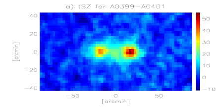
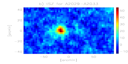
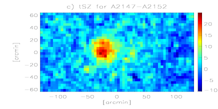
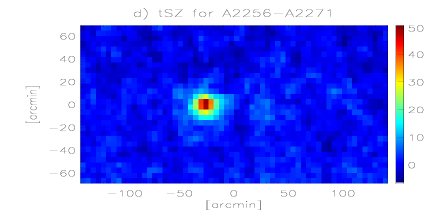
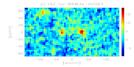
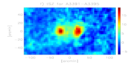
Figure 1: MILCA maps of the Compton parameter $y\times 10^{6}$ for the selected pairs of clusters. From left to right and from top to bottom we show the pairs of clusters a) A0399-A0401, b) A2029-A2033, c) A2147-A2152, d) A2256-A2271, e) MKW 3s-A2063, f) A3391-A3395 and g) A0209-A0222.

In the region trapped between interacting pairs of clusters we expect a hotter and denser phase of the WHIM (see Section 1) that might produce enough SZ emission to be detected by the Planck satellite. The combined full sky capabilities, lack of atmospheric fluctuations, and wide frequency coverage makes Planck a unique instrument to study these peculiar objects.

To identify pairs of merger clusters in the Planck maps we used the MCXC catalogue of clusters, Piffaretti et al. (2011), which provides the main physical parameters of X-ray detected clusters of galaxies (position, redshift, angular extension $\theta_{500}$, and mass $M_{500}$). We selected a sample of cluster pairs whose difference in redshift is smaller than 0.01 and whose angular distance is between 10 and 120^′. For all selected pairs we constructed maps of the tSZ (tSZ hereafter) emission from the Planck HFI frequency maps at a resolution of 7.18^′ using different component separation techniques: MILCA (maximum internal linear component analysis, Hurier et al. (2010)), NILC (needlet internal linear combination, Remazeilles et al. (2011)) and GMCA (generalized morphological component analysis, Bobin et al. (2008)). A detailed discussion of the relative performance of these component separation techniques can be found in Planck Collaboration et al. (2012) and Melin et al. (2012). Below we take the MILCA maps as a reference to simplify the discussion. The tSZ maps are centred on the barycentre of the X-ray position of the two clusters and extend the distance between the two clusters (as given in the MCXC catalogue) by up to five times. The error distributions on the final SZ maps were computed using the Planck jack-knife maps described in Planck HFI Core Team et al. (2011).

Using these tSZ maps, we finally selected those pairs of clusters for which at least one of the clusters has a signal-to-noise ratio higher than five. Table 1 shows the position (in Galactic coordinates), the redshift, and the angular diameter (in $\theta_{500}$ units) of the two clusters as well as the angular distance between them (in arcminutes) for each of the selected pairs of clusters. We divided the selected clusters into three different sets (separated by horizontal lines in Table 1). The first set corresponds to the pairs of clusters for which both clusters are significantly detected in SZ by Planck. The second set corresponds to the pairs for which one of the clusters is only marginally detected in SZ by Planck. The third set consists of pairs of clusters separated by less than 30 ^′. After a first assessment we concluded that for the last two sets the modelling of the clusters in the pair is too complex, given the lower significance of the data. This makes it difficult to extract reliable information on the intercluster region, therefore we do not consider them further in the analysis presented in the next sections.

Figure 1 shows maps of the Compton parameter $y\times 10^{6}$ for the six pairs of clusters in the first group in Table 1 (in decreasing order of $y$ from a) to f) ). These maps are rotated so that the virtual line connecting the centre of the clusters is horizontal and at the middle of the figures. The direction defined by this line is called longitudinal hereafter, and the direction perpendicular to it is called radial. The pixel size in the longitudinal and radial directions is defined by the angular distance between the centre of the two clusters, $d$, as follows: $\theta_{pix}=5\times d/60$. From visual inspection of these maps we infer that there might be significant SZ emission in the intercluster region of the pairs of clusters A399-A401, A2147-A2152, MKW 3s-A2063, and A3391-A3395. To confirm these findings we computed 1D longitudinal profiles by stacking the above maps in the radial direction. Figure 2 shows the 1D profiles for the six pairs of clusters (notice that the errors are correlated). The figure also shows the residuals after subtracting an estimate of the tSZ emission from the clusters. In the intercluster region we simply used a symmetric interpolation (in red in the figure) of the external profile of each of the clusters. When there was an obvious contribution from extra clusters (see for example the shoulders on the A3391-A3395 pair, Figure 2e) and the peak on the A2029-2033 pair, Figure 2b), we excluded the affected region from the analysis. The error bars on the residuals are increased by a factor $\surd 2$ in the outskirts and $\surd 3$ in the intercluster region to account for the interpolation, symmetrization, and subtraction. We observe clear extra emission for two of the pairs: A399-A401 (Figure 2a) and A3391-A3395, (Figure 2e). In the intercluster region, $\chi^{2}$ for the null hypothesis (no extra tSZ signal) is 20 for A399-A401 and 174 for A3391-A3395, for eight degrees of freedom (11 data samples minus 3 parameters). We also found high $\chi^{2}$ values for the A2029-A2033 (Figure 2b) and A2256-A2271 (Figure 2d) pairs of clusters. However, for these two pairs we observe a deficit of tSZ signal in the intercluster region that is induced either by an over-estimation of the tSZ emission of the clusters themselves or by their asymmetric geometry. Therefore, we only considered the A399-A401 and A3391-A3395 pairs of clusters for further analysis because they show the most prominent tSZ signal in the intercluster region. To check that the excess of tSZ effect observed cannot be explained by contamination by foreground emissions (Galactic), we estimated the dust temperature using Planck and IRAS data and a simple modified blackbody SED that we fitted to the Planck+IRAS data. No strong deviations in the temperature that could compromise the component separation process were observed in the field of view.

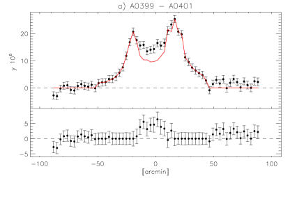
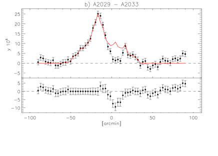
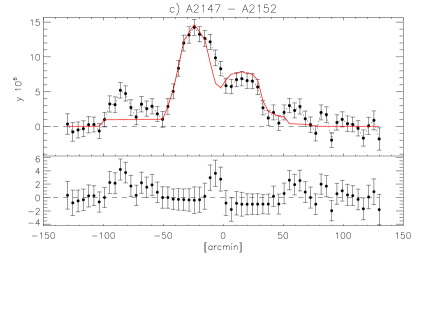
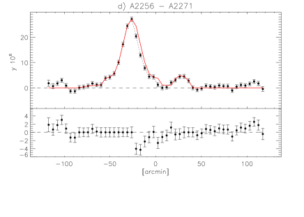
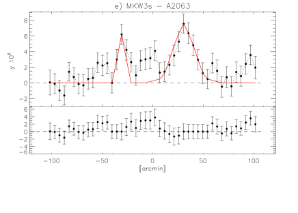
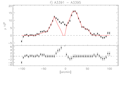
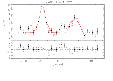
Figure 2: Like in figure 1. From left to right and from top to bottom, 1D tSZ longitudinal profiles and residuals after subtracting the contribution from the clusters (see text for details) for the pairs of clusters a) A399-A401, b) A2029-A2033, c) A2147-A2152, d) A2256-A2271, e) MKW 3s-A2063, f) A3391-A3395, and g) A0209-A222.

4 X-ray data for the selected pairs

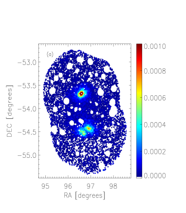
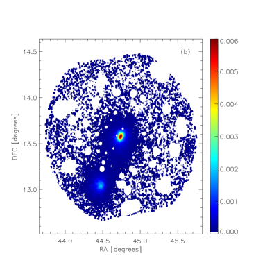
Figure 3: Maps of the X-ray emission (in counts per second) for the cluster pairs a) A3391-A3395 and b)A399-A401.

To improve the quality of our analysis we complemented the Planck data with X-ray observations retrieved from the ROSAT archive. Our choice of using ROSAT/PSPC is motivated by i) its ability to detect the faint surface brightness emission (i.e the cluster emission at large radii Vikhlinin et al. (1999); Eckert et al. (2011) and the intercluster region in superclusters (Kull & Böhringer, 1999)), ii) its large field of view ($\sim$2  deg²) and iii) the low instrumental background. These factors make ROSAT/PSPC the X-ray instrument that is most sensitive to diffuse low surface brightness emission. On the negative side, its limited bandpass and poor spectral resolution is not best-suited for measuring plasma temperatures.

We used the ROSAT extended source analysis software (ESAS, Snowden et al. (1994)) for data reduction, following the procedure in Eckert et al. (2011). We produced images of the counts in the R37 ROSAT band, i.e. in the energy range $0.42-2.01$  keV, and corrected for vignetting effects through the exposure map produced with the ESAS software. Following Eckert et al. (2011), we detected point sources up to a constant flux threshold, to resolve the same fraction of the CXB on the entire field of view (FOV). We estimated the sky background components in the fraction of the FOV not contaminated by cluster emission ($r>1.3r_{200}$) and then subtracted this constant value from the image. Error bars for the count rate were estimated by propagating Poissonian errors of the original source and background count images.

The ROSAT/PSPC point spread function (PSF) strongly depends on the position in the FOV, ranging from 15^′′ on axis to 2^′ in the outer parts of the FOV. We considered an average PSF representative of our data sets as computed assuming a position 1^′ off axis and having 1  keV energy. We checked that variations within reasonable limits ($E=0.5-2$ keV and off axis = 0-10 arcmin) do not introduce significant changes in our results. To reduce statistical noise we smoothed the X-ray data with a 2^′ Gaussian kernel. The scale of this smoothing is significantly smaller than Planck’s angular resolution, so it does not compromise the results derived from X-ray data. This also helps to make the uncertainties in the ROSAT PSF a second-order effect.

Since we used PSPC archive data and covered regions that might be larger than the FOV of ROSAT, we needed to combine different pointings into a single mosaic. The pair A399-A401 (Figure 3a) is contained in a single PSPC pointing, therefore in principle it is not necessary to perfomr a mosaic here. However, we still combined the neighbouring pointing rp800182n00 and rp80235n00, to increase the statistics. The total combined exposure time is $\sim 14$  ks. For A3391-A3395 (Figure 3b), the larger separation in the sky between the clusters, forced us to combine at least two pointings. We combined the two available observations for this pair: rp800079n00 ($2.5$  ks centred on A3395) and rp800080n00 (6  ks centred on A3391). The final X-ray maps in counts per second are presented in Figure 3.

5 Modelling of the tSZ and X-ray emission from the clusters

One of the key problems of the analysis presented in this paper is estimating the tSZ and X-ray emission of the clusters themselves because this estimate is later used to remove the contribution of the clusters from the intercluster region. In this section we present a detailed description of modelling the cluster emission for the A399-A401 and A3391-A3395 cluster pairs.

5.1 tSZ and X-ray emission from clusters

When CMB photons cross a galaxy cluster, some of the photons will probably interact with the free electrons in the hot plasma through inverse Compton scattering. The temperature decrement (increment for frequencies $\nu>217$  GHz) observed in the direction $\theta$ can be described as

$$\Delta T(\theta)=T_{o}\int n_{e}(l)T(l)dl,$$ (1)

where $T_{o}$ contains all relevant constants, including the frequency dependence ($g_{x}=x(e^{x}+1)/(e^{x}-1)-4$ with $x=h\nu/kT$), $n_{e}$ is the electron density and $T$ is the electron temperature. The integral is performed along the line of sight. The quantity $P(l)=n_{e}(l)T(l)$ is often referred to as the pressure produced by the plasma of thermal electrons along the line of sight.

We can also consider the thermal X-ray emission from the hot ionized plasma including bremsstrahlung and line- and recombination emission from metals given by

$$S_{x}(\theta)=S_{o}\frac{\int n_{e}^{2}\lambda(T)dl}{D_{l}(z)^{2}},$$ (2)

where $D_{l}(z)$ is the luminosity distance. The quantity $S_{o}$ contains all relevant constants and corrections (including the band- and k-corrections). By combining X-ray and SZE observations it is in principle possible to break the degeneracy between different models because of their different dependency on $T$ and specially on $n_{e}$.

5.2 Pressure profile models

The tSZ and X-ray emission of clusters can be computed from the density and temperature profiles of the thermal electrons in the cluster. Below we describe the models of the electron pressure profiles for clusters that were used to estimate and subtract the cluster contributions from the pairs of clusters.

$\beta$-model

The isothermal $\beta$-model is historically the most widely used in the literature in the context of galaxy clusters. Even if cluster observations have shown that this model is over-simplified and unable to describe the details of the intercluster medium (ICM) distribution, it allows us to use a limited number of parameters to produce a useful first approximation of the radial behaviour of the gas. Indeed, we are not interested in the details of the single objects, but in removing the main signal coming from the two clusters in the system to study the SZ excess signal observed between them by Planck. In the isothermal $\beta$-model, the electron temperature is assumed to be constant and its density is given by

$$n_{e}(r)=n_{e0}\left(1+\frac{r^{2}}{r_{c}^{2}}\right)^{\frac{-3\beta}{2}},$$ (3)

where $n_{e0}$ is the central electron density and $r_{c}$ is the core radius.

Generalized Navarro Frenk and White pressure profile

Given the characteristic pressure P₅₀₀, defined as

$$P_{500}=1.65\cdot 10^{-3}h(z)^{8/3}\left[\frac{M_{500}}{3\cdot 10^{14}h_{70}^{-1}}M_{\odot}\right]^{2/3}h_{70}^{2}\thinspace keV\thinspace cm^{3},$$ (4)

the dimensionless universal (scaled) pressure profile can be written as (Nagai et al., 2007; Arnaud et al., 2010)

$$\mathds{P}(x)=\frac{p_{o}}{\left(c_{500}x\right)^{\gamma}\left[1+\left(c_{500}x\right)^{\alpha}\right]^{\left(\beta-\gamma\right)/\alpha}},$$ (5)

in which $x=r/R_{500}$, $c_{500}=R_{500}/r_{s}$, and $\gamma$, $\alpha$ and $\beta$ are the central ($r<<r_{s}$), intermediate ($r\sim r_{s}$) and outer ($r>>r_{s}$) slopes. The radial pressure can be the expressed as

$$P(r)=P_{500}\mathds{P}(x),$$ (6)

with $[p_{o},c_{500},\gamma,\alpha,\beta]=[8.403h_{70}^{-3/2},1.117,0.3081,1.0510,5.4905]$, as derived by Arnaud et al. (2010). For the sake of simplicity, we redefine the normalization as $P_{0}=P_{500}*p_{o}$, also in units of $keV\thinspace cm^{3}$. As a result of the anticorrelation of the density and temperature profiles, at cluster cores the pressure exhibits less scatter than the electron density and temperature, and is accordingly better suited to define a universal profile. However, in the core region, the dispersion about the average profile found by Arnaud et al. (2010) is still significant ($\sim$ 80 % at 0.03 $R_{500}$), while it becomes less than 30% beyond 0.2 $R_{500}$.

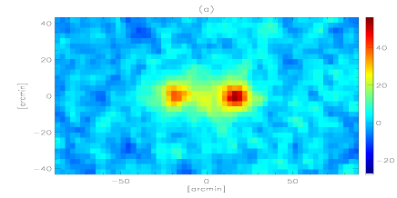
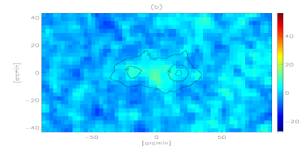
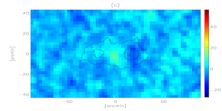
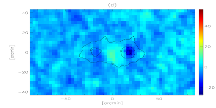
Figure 4: a) Planck tSZ Compton parameter map ($y\times 10^{6}$); b) residuals after subtracting of the GNFW2 model; c) residuals after subtracting of the GNFW1 model; and d) residuals after subtracting of the $\beta$ model of the clusters as described in the text.

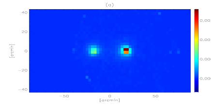
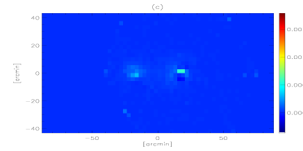
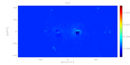
Figure 5: X-ray data and residuals of the best-fit cluster model for the A399 and A401 pair of clusters. a) ROSAT map; b) residuals for the GNFW2 model; c) residuals for the GNFW1 model; and d) residuals for the $\beta$ model.

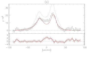
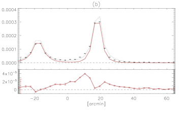
Figure 6: 1D a) tSZ and b) X-ray profiles and residuals for the best-fit models of the A399 and A401 clusters. The red curve corresponds to the GNFW2 model. The dotted lines are the model from Sakelliou & Ponman (2004).

5.3 Fitting the tSZ and X-ray emissions from the clusters

We used the $\beta$ and generalized Navarro Frenk and White (or GNFW hereafter) pressure profile models to fit the tSZ and X-ray emissions of the clusters in the A399-A401 and A3391-A3395 pairs. For the $\beta$-model we varied the central density, $n_{o}$, the slope $\beta$, and the core radius $r_{c}$ of each cluster. For the GNFW model we considered two different sets of models: GNFW1 and GNFW2. For the first one, we fixed $\beta=3.5$ and fitted the other parameters. For the second one, $c_{500}$, $\gamma$ and $\alpha$ were fixed to the Arnaud et al. (2010) values, leaving $P_{0}$ and $\beta$ free to vary.

We fitted each cluster individually excluding the intercluster region from the fit. For the tSZ emission we integrated the pressure profile along the line of sight up to $5\times R_{500}$ (unless stated otherwise) following equation 1. The resulting map was convolved with a Gaussian beam of 7.18^′ to match the resolution of the MILCA SZ map. For the X-ray emission we considered an isothermal scenario and computed the electron density from the pressure profile. We then used equation 2 to compute the surface brightness of the clusters. An X-ray map in counts per second was obtained from the latter using the MEKAL model (Mewe et al., 1985, 1986; Kaastra, 1992; Liedahl et al., 1995) for cluster emission and the WABS model (Morrison & McCammon, 1983) for absorption of the neutral hydrogen along the line-of-sight. The MEKAL model is a function of the square of the electron density, the temperature, and the redshift of the cluster. The WABS model uses column density maps (Dickey & Lockman, 1990; Kalberla et al., 2005). We convolved the final X-ray map with a Gaussian beam of 2^′ to match the resolution of the 2^′ resolution (degraded) ROSAT map.

We performed different fits including X-ray data only, SZ data only, and both X-ray and SZ data. The fits were performed directly on the 2-D maps presented above and correlated errors were accounted for in the likelihood analysis. For the joint tSZ and X-ray fits the likelihood functions were normalized by their volume and then multiplied to obtain the best-fit parameters and errors.

Results for the A399-A401 pair

Table 2: Best-fit parameters for the pressure profile $\beta$-model. For this analysis KT and $R_{max}$ were fixed to the values shown.

        Cluster         $$\beta r_{c} {}^{-}3 R_{max} 2.37\times 10^{-3} 5.50\times 10^{-3} 2.61\times 10^{-3} 1.17\times 10^{-3} 1.17\times 10^{-3}$$          (kpc)         n₀ (cm)         KT (keV)          (kpc)         A399         0.928         432.8                  7.23         2160         A401         0.928         298.4                  8.70         2340         A3391         0.620         213.0                  6.00         1500         A3395SW         0.673         328.0                  4.80         1400         A3395E         0.726         356.6                  5.00         1200

Table 3: Best-fit parameters for the GNFW1 pressure profile model. For this analysis $\beta$ and KT were fixed to the values shown.

     Cluster      c₅₀₀      $$\gamma \alpha \beta \times 10^{-2} \times 10^{-2} \times 10^{-2} \times 10^{-2} \times 10^{-2}$$                  r₅₀₀ (Mpc)      P₀ (keV / cm³)      kT (keV)      A399      1.80      0.000      1.25      3.5      1.11      2.04      7.23      A401      2.58      0.016      1.59      3.5      1.24      3.76      8.47      A3391      0.69      0.033      0.72      3.5      0.90      3.08      6.00      A3395SW      2.65      0.066      2.00      3.5      1.10      0.70      4.80      A3395E      0.3      0.000      0.58      3.5      0.90      1.89      5.00

Table 4: Best-fit parameters for the GNFW2 pressure profile model. For this model c₅₀₀, $\gamma$, $\alpha$ and r₅₀₀ were fixed to the values shown.

     Cluster      c₅₀₀      $$\gamma \alpha \beta \times 10^{-2} \times 10^{-2} \times 10^{-2} \times 10^{-2} \times 10^{-2}$$                  r₅₀₀ (Mpc)      P₀ (keV cm³)      kT (keV)      A399      1.18      0.308      1.05      3.5      1.11      0.97      5.0      A401      1.18      0.308      1.05      5.0      1.24      2.40      6.5      A3391      1.18      0.308      1.05      3.5      0.89      0.75      6.0      A3395SW      1.18      0.308      1.05      3.5      0.93      0.40      4.8      A3395E      1.18      0.308      1.05      3.5      0.93      0.40      5.0

We converted the density profile into ROSAT PSPC count rates, using an absorbed MEKAL model within XSPEC (Arnaud, 1996). The conversion rate was computed using the temperatures in Sakelliou & Ponman (2004), a metal abundance $Z=0.2$ solar, the Galactic column density in the direction of the pair $nH=1.09\times 10^{21}\thinspace\rm{cm}^{-2}$ (Dickey & Lockman, 1990) and the redshifts $z=0.0737$ for A401 and $z=0.0724$ for A399. We fixed the truncation radius in the 3-D integrals to the $r_{200}$ value in Sakelliou & Ponman (2004) (this choice is not mandatory provided the radius is reasonably large).

Before model fitting, we used three different methods to estimate the background or zero level of the tSZ Compton parameter maps. The results are consistent between the three methods. The first method computes the mean signal in an area around the cluster pairs that excludes the pairs. This region does not show any other source that needs to be masked out. The second method computes the mean signal of the averaged profiles of the clusters beyond R200 and in the directions opposite to the other cluster. The third method computes a histogram of the background region defined in the first method and finds the median of the distribution. We adopted method one for the final results.

Tables 2, 3, and 4 present the best-fit parameters of the A399 and A401 clusters for the $\beta$, GNFW1, and GNFW2 pressure profile models. The residual tSZ maps for these best-fit cluster models are shown in Figure 4. We note that for the GNFW2 pressure profile model (Figure 4d) the derived temperatures are lower than those derived from X-ray-only data and in particular with the results from XMM-Newton by Sakelliou & Ponman (2004). For the other two models the temperatures were fixed to the Sakelliou & Ponman (2004) value. We show the Planck tSZ map (Figure 4a) and the residuals after subtracting the best-fit $\beta$ model (Figure 4b) and the best-fit GNFW model for the two sets described above (Figure 4c and 4d). In the residuals we clearly observe an excess of tSZ emission with respect to the background. This can also be observed in Figure 6a) where we present the 1D tSZ longitudinal profile and residuals for the GNFW2 model described before and for the Sakelliou & Ponman (2004) best-fit model .

In Figure 5 we show the ROSAT X-ray maps for the A399 and A401 clusters and the residuals after subtracting the $\beta$, GNFW1 and GNFW2 models. We observe that the models slightly under-estimate the signal at the centre of the clusters. This is also seen in Figure 6b) where we present the 1D x-ray longitudinal profile and residuals for the three pressure profile models. A similar behaviour was observed when fitting XMM-Newton data in Sakelliou & Ponman (2004). Quoting Sakelliou & Ponman (2004), “neither of the two central galaxies is known to host an active nucleus, whose presence could be invoked to explain the requirement for an extra, but small, central component”. For illustration we also plot (dotted lines) the best-fit model of the clusters found by Sakelliou & Ponman (2004). This model clearly over-predicts the tSZ cluster emission. However, this discrepancy is not surprising, given the different dependencies of the SZ and X-ray signals on the ICM density and temperature. Indeed, as pointed out by Hallman et al. (2007), the inadequacy of the isothermal assumptions affects the parameter determination performed on SZ and X-ray data in a different way, therefore X and SZ profiles cannot be represented properly using the same parameter values for an isothermal $\beta$-model. Isothermal $\beta$-models derived from X-ray observations, in general, overpredict the SZ effect and steeper profiles are needed to simultaneously fit SZ and XR data (e.g. (Diego & Partridge, 2010)). Other factors that affect the SZ and XR in different ways are for instance clumpiness and triaxiality that can be invoked to explain part of the discrepancy, as we discuss below. The different sensitivity to the details of temperature and gas density distribution is still relevant even when comparing integrated quantities such as $Y$, the integrated Comptonization parameter, and the proxy $Y_{X}=k_{B}TM_{gas}$, (Kravtsov et al., 2006), whose ratio has been found to be lower than 1 by several different authors (Arnaud et al. (2010); Planck Collaboration et al. (2011c); Andersson & SPT Collaboration (2010); Rozo et al. (2012)). This agrees with our findings and confirms the importance of a joint X-ray/SZ analysis, which is able to break the degeneracy between models. Nevertheless, despite the uncertainties in the central part of the clusters, we observe an excess of X-ray and tSZ signal in the intercluster region. This excess is discussed in section 6.

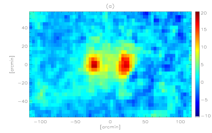
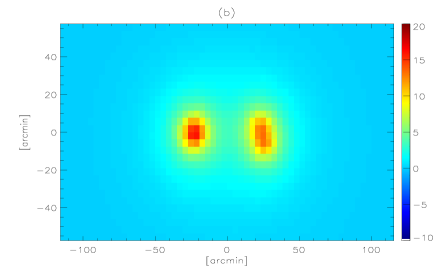
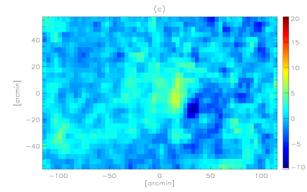
Figure 7: a) tSZ Compton parameter map ($y\times 10^{6}$), b) best-fit model of the clusters, and c) residuals after subtracting the best fit model for the A3391 and A3395 pair of clusters.

Results for the A3391-A3395 pair

Modelling the A3391 and A3395 pair is a challenging task. A3395 is a multiple system formed of at least three identified clusters (see Tittley & Henriksen (2001)). For the purpose of this paper we considered the two clusters most important in X-rays (SW and E), which can be clearly identified in Figure 3. The quality of the X-ray data is significantly poorer than in the case of A399-A401 (less than half the amount of exposure time), making it difficult to distinguish between background and diffuse X-rays in the intercluster region. Moreover, the clusters that form the system A3395 are clearly elongated (this is even clearer when studying XMM-Newton and Chandra  images of the cluster, see for example Tittley & Henriksen (2001)), which adds another complication to the model. For the SZ part of the data, even though there seems to be a signal in the intercluster region, the modelling of the SZ signal from A3395 is affected because Planck cannot resolve the individual subsystems in A3395. Despite all these complications, we are able to perform a basic fit to the SZ and X-ray data. The best-fit parameters for the three pressure profile models are presented in the last three rows of tables 2, 3, and 4. We show in Figure 7 a) the tSZ Planck map for the A3391-A3395 pair, b) the best-fit GNFW2 model, and c) the residuals after subtracting this model. We clearly observe in the residuals a significant excess of signal in the region near the A3395 system. Indeed, the integrated Compton parameter in the intercluster region is $Y=(4.5\pm 0.7)\ 10^{-3}$ (arcminutes)² –of the same order of magnitude as that for the A399-A401 pair (see below). However, this residual is suspiciously close to the NW component of the A3395 cluster that was discussed in Tittley & Henriksen (2001) (and not included in our model), indicating that a far more complex model is necessary to subtract the cluster components. We can also notice in the figure the contribution from a radio point-source that appears as a decrement in the reconstructed Compton parameter map. The area contaminated by this point source was excluded from the analysis. Due to the uncertainties in the model and in the foreground subtraction (radio point source contribution), the analysis of the intercluster region gives unreliable constraints on the density and temperature of this region and is not considered in the following analysis.

6 Analysis of the intercluster residuals

6.1 Models

To model the intercluster region of the pair of clusters we considered either an extra background cluster or a filament-like structure described by a parametric model.

Extra cluster

In this case we assumed a background cluster in the intercluster region of the pair. To simplify the modelling, we considered that the cluster properties are fully defined by its redshift and $M_{500}$ mass, which are the free parameters of the model. From M₅₀₀ we computed $R_{500}$ and used scaling relations to compute the temperature. We finally assumed that the pressure profile of the cluster is well described by a universal profile and used the parameters obtained by Arnaud et al. (2010) for cool cores discussed in the previous section.

Filament-like structure

In this case we assumed that the intercluster region can be described by a tube-like filament orientated perpendicularly to the line of sight. We considered an isothermal filament of temperature T. For the electron density we considered two cases, one in which the density remains constant inside the tube and another in which the density falls from a maximum to zero in the border of the tube. The main physical parameters are the normalization density, the temperature of the filament, and its radius. For the latter the electron density profile is defined in the radial direction in cylindrical coordinates as follows

$$n_{e}(r)=\frac{n_{e}(0)}{\left(1+(\frac{r}{r_{c}})^{2}\right)^{\frac{3}{2}\beta}},$$ (7)

with $\beta=2/3$ and $r_{c}=10$^′. The free parameters of the model are the temperature, $T$, and the central electron density, $n_{e}(0)$.

6.2 A399-A401

From the three models considered in the previous section, we computed the residual signal in tSZ and X-ray. The amount of signal in the intercluster region was then used to constrain the parameters of the extra cluster or the filament. For the case of an extra cluster behind the intercluster region we obtain the results in Figures 8 a) and c) where we trace the 1D and (Figure 8b) 2-D likelihood contours at 68%, 95.5%, and 99% confidence level for z and $M_{500}$. Only clusters at high redshift $z=1.95$ and with a large mass $M_{500}=2.4\times 10^{15}M_{\circ}$ will be capable of producing a strong enough SZ signal with the strength of our Planck residual but with X-rays that do not exceed the ROSAT signal. These results are not consistent with existing constraints on structure formation, which predict that massive clusters are formed at low redshifts (see for example Figure 2 in Harrison & Coles (2012).

Figure 8: Constraints on the redshift and $M_{500}$ for an extra cluster in the intercluster region of the A399-A401 system.

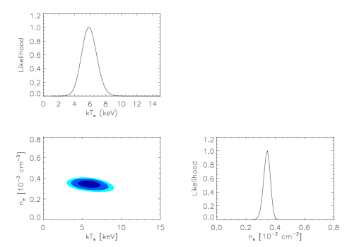
Figure 9: Constraints on the temperature and density of the filament in the intercluster region of the A399-A401 system. A high temperature $\sim 7$ keV is also favoured by the XMM data (Sakelliou & Ponman, 2004).

The best-fit parameters in the filament case are presented in Figure 9 where we show the 1D and 2-D likelihood contours at 68%, 95.5%, and 99% confidence level for T and $n_{e}(0)$. We find that the temperature of the filament is $(7.08\pm 0.85)$  keV and the central electron density is $(3.72\pm 0.17)\ 10^{-4}$  cm^-3. These results are consistent with previous estimates by Sakelliou & Ponman (2004). It is interesting to look at the residuals for the best-fit clusters (we used the GNFW2 model here) and the filament model. Figure 10 shows the 1D longitudinal profiles and residuals for the tSZ effect and X-ray emission after subtracting the clusters and filament models. We observe that the excess of tSZ effect in the intercluster region is well described by the filament model. The integrated Compton parameter in the intercluster region is $Y=(6.1\pm 0.7)\ 10^{-3}$  arcmin².

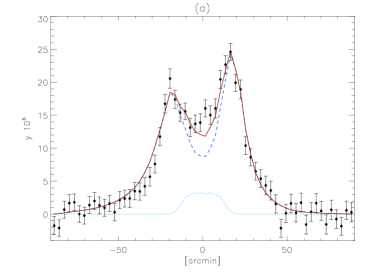
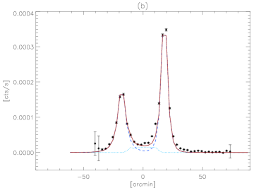
Figure 10: a) tSZ longitudinal profile and b) X-ray longitudinal profile. Data from Planck  and ROSAT (black points), from the total model (red line), the PXCC model only (light blue line), and the filament model only (dark blue line).

7 Comparison with hydrodynamical simulations

We applied the full analysis described in the previous sections to hydrodynamical simulations of a supercluster-like region  (Dolag et al., 2006) that mimic our cluster pairs. Unlike the original simulations presented in  Dolag et al. (2006), this simulation was carried out including the treatment of radiative cooling, heating by a uniform UV background and star formation feedback processes based on a subresolution model for the multiphase structure of the interstellar medium (Springel & Hernquist, 2003). The simulation also follows the pattern of metal production from the past history of cosmic star formation (Tornatore et al., 2004, 2007). This is done by computing the contributions from both type-II and type-Ia supernovae. Energy is fed back and metals are released gradually in time, according to the appropriate lifetimes of the different stellar populations. This treatment also includes, in a self-consistent way, the dependence of the gas cooling on the local metallicity. The feedback scheme assumes a Salpeter initial mass function (IMF) (Salpeter, 1955) and the parameters were fixed to obtain a wind velocity of $\approx 480\thinspace km\thinspace s^{-1}$.

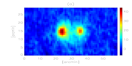
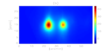
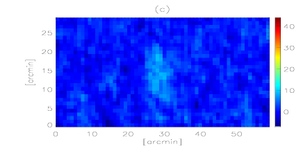
Figure 11: a) tSZ Compton parameter map ($y\times 10^{6}$) for Halo b in the hydrodynamical simulations, b) best-fit model for the clusters in the pair, and c) residuals after subtracting the latter.

We concentrated our analysis on a system of two merging clusters with characteristics similar to the A399-A401 system. In the simulation, a cluster with a virial mass of $6.5\times 10^{14}$ $M_{\odot}$/h (Halo d) is merging with a cluster with a mass of $1.1\times 10^{15}$ $M_{\odot}$/h (Halo b). At $z=0.07$ the two systems are physically separated by 4 Mpc/h (2.9 Mpc/h in the projection shown in figure 12), which compares remarkably well with the A399-A401 system, where the projected separation of the systems is $\sim 3$  Mpc. More details on the appearance and the geometry of the simulated system can be found in  Dolag et al. (2006). Figure 11 shows the Compton parameter maps (multiplied by 10⁶). After subtracting the best-fit model for the clusters (Figure 11b), we fitted the residuals (Figure 11c)) in the intercluster region with the filament model described above. For the best-fit model of the filament the integrated Compton parameter is $Y=(3.5\pm 0.7)\times 10^{-3}$  arcmin² and agrees well with the input $Y_{input}=3.2\times 10^{-3}$  arcmin². It is also important to notice that the error bars obtained are consistent with those obtained for the cluster pair A399-A401.

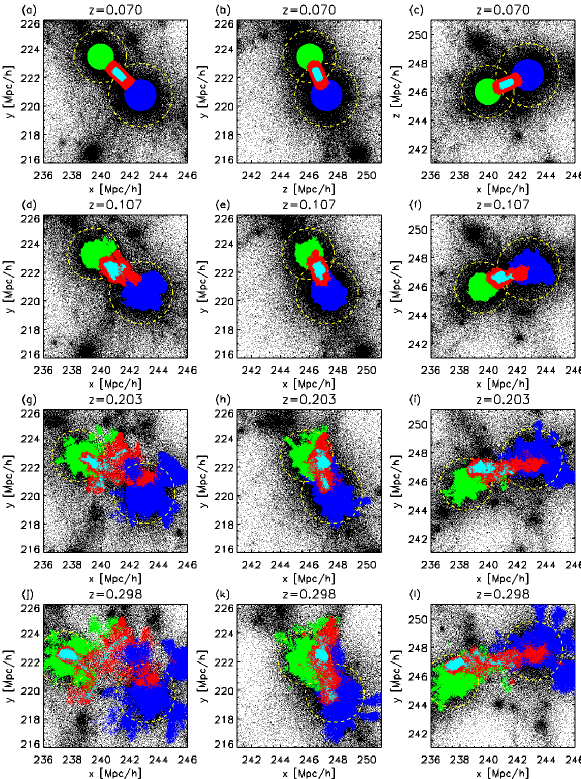
Figure 12: Spatial projections (along x,y and z axis) of the particles in the simulation. The rows show the simulation at z=0.07, z=0.1, z=0.2 and z=0.3 respectively. We colour code the particles depending on their location: clusters (green/blue), the filamentary region in between (red) and the central part of this filament (cyan). See text for a more detailed definition. Additionally the yellow circles mark the virial radius of the two clusters.

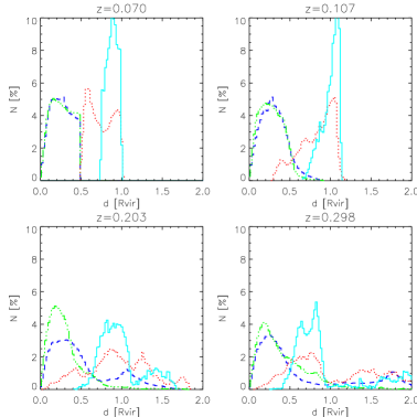
Figure 13: Evolution of the radial distribution of the particles with respect to the centre of the closest of the two clusters. The colour code is the same as in figure 12. The dashed and dot-dashed lines correspond to the blue and green particles (clusters) while the dotted and solid lines orrespond to the red and cyan particles (filament).

We traced the origin of the particles causing the signal within the region between the two clusters. To do this, we distinguished between particles belonging to the main part of one of the two galaxy clusters (e.g. within 0.5 R_vir ) and the particles belonging to the filament, selected as those particles within a cylinder of 1Mpc/h in diameter between the two clusters and lying outside 0.5 R_vir. Additionally, we defined particles in the central part of the filament as those within a cylinder of 0.5 Mpc/h in diameter between the two clusters and lying outside 0.75 R_vir. Figures 12 a-c show the different location of the particles colour-coded in blue and green for particles belonging to the clusters, red for particles in the filament, and cyan for those in the inner part of the filament. The yellow circles mark the virial radius of the two clusters. Going back in time to z=0.1, z=0.2, and z=0.3 (corresponding to 0.4, 1.5 and 2.5 Gyr) reveals the spatial origin of these particles. We can observe that according to the origin of these particles, the intercluser region at z=0.07 is populated by two separate components. One component is coming from material that belonged to the outer atmosphere of one of the two clusters at z=0.3, and the other one is coming from a very diffuse structure, outside but connecting both clusters. This structure has a sheet-like geometry at early times. When we trace back the origin of the particles in the very central part of the filament, most of the particles were farther than 0.5 R_vir from one of the main clusters within the last 2.5 Gyr. This is made more evident in Figure 13, which shows the spatial distribution of the particles of the different components more quantitatively. Here we sorted each particle by its shortest distance to either cluster. When we concentrate our attention on the filament’s core (light blue particles), only a very small fraction of the particles in this region were closer than 0.5 R_vir to one of the two main halos at z=0.3. More than half of them are coming from regions with 0.5 R${}_{vir}<$ R $<$ R_vir and a considerable fraction is coming from regions beyond R_vir.

This simulation shows that the intercluster region might be populated by a mix of components from both the clusters and the intergalactic medium.

8 Discussion

The significant SZ signal between pairs of clusters combined with the lack of significant X-ray signal suggestes that merging events may have occurred, leaving filaments of matter between these interacting pairs. Merging of the clusters would contribute to the increased pressure that boosts the SZ signal. These results qualitatively agree with hydrodynamical simulations in which the intercluster region between an interacting pair of clusters can show significant SZ signal (Dolag et al., 2006).

Regarding the cluster pair A399-A401, earlier studies showed that the intercluster medium in this pair is compressed by the merging process (Fujita et al. (1996), Sakelliou & Ponman (2004)). The increased pressure would increase the SZ signal. Akahori & Yoshikawa (2008) studied the non-equilibrium state of this system with simulated data and found that there might be significant shock layers at the edge of the linked region between the clusters that could explain a boost in the SZ signal. Also, Suzaku  observations found that the intercluster medium has a relatively high metallicity of 0.2 solar (Fujita et al. (2008)). These works estimated that the filamentary bridge would have an electron density of $n_{e}\sim 10^{-4}$ cm^-3 (Fujita et al. (1996), Sakelliou & Ponman (2004), Fujita et al. (2008)).
Given that the angular separation between the two clusters is $\sim 3$ Mpc and that both clusters are at slightly different redshifts (0.0724 and 0.0737), we can assume that the clusters are not exactly on the same plane of the sky and that their true separation is larger than 3 Mpc. That is, the clusters would be separated by more than their respective virial radii. Consequently we can conclude that the signal (or at least a significant percentage of it) seen by Planck in the intercluster region corresponds to baryons outside the clusters.

Our results show that there is evidence for a filamentary structure between the pair A399-A401 and outside the clusters, but the results also raise some questions about the origin of this gas. The uncertainties in estimating the cluster contributions around their virial radii makes it difficult to distinguish between the different scenarios. In a pre-merger scenario a filament could have been trapped in between the clusters, with its material being reprocessed and compressed as the clusters approach each other. In a post-merger scenario (by post-merger we mean not direct crossing of the cluster cores but a gravitational interaction as the two approaching clusters orbit their common centre of mass), the intercluster signal could be just the result of the overlapping tails of the disturbed clusters.

These clusters could be elongated due to their gravitational interaction, or a bridge of matter may have formed between the clusters after an interaction. The fits to SZ and X-Ray data reveals that there are some apparently conflicting results, which make it harder to reconcile the SZ and X-ray data with spherical, standard models. A good example is the best-fitting model of Sakelliou & Ponman (2004) that over-predicts the SZ data. This could be, for instance, an indication that spherical models may not be the most appropriate for describing these clusters. The failure of the Sakelliou & Ponman (2004) model to properly describe the Planck data shows how Planck data can be used to add information on the third dimension.

Non-sphericity is expected (and indeed observed) in X-rays and could introduce corrections to the best-fitting models, particularly if the elongations of the clusters point towards each other (as is the case for A401 from the X-ray images). In this case, the gas density in the intercluster region would be enhanced due to this elongation. Sereno et al. (2006) showed how clusters seem to favour prolate geometries. A prolate model would increase the X-ray signal for the same number of electrons (or SZ), or vice versa, the same X-ray signal requires fewer electrons (or SZ). We estimated that a ratio of $\sim 1.3$ between the axis might be sufficient to reduce the SZ signal by $\sim 30\%$ with a fixed X-ray observation (i.e, fixing the other two axes and the total X-ray signal).

Clumpiness is another factor that might be introducing a bias in the models that best subtract the cluster components. Mathiesen et al. (1999) used simulations to estimate the mean mass-weighted clumping factor $C=<n^{2}>/<n>^{2}$. They found typical values for $C$ between 1.3 and 1.4 within a density contrast of 500. Since for an isothermal model $C$ can be seen as the ratio of X-ray to SZ signal (squared), as in the case of prolate clusters discussed above, clumpiness of the gas would increase the X-ray signal for the same number of electrons (or SZ) or vice-versa, the same X-ray signal would require fewer electrons (or SZ).

One cluster will have an effect on the other cluster and in the intercluster region through its gravitational potential. Figure 14 shows the resulting gravitational field across the line intersecting the two cluster centres. The gravitational field is computed from the hydrostatic equilibrium equation assuming a profile of the gas density (and a constant temperature). We use one of our best-fitting models described earlier (universal profile) for this purpose. The intercluster region shows a significant enhancement in the gravitational potential. The effect is more significant in A399 where the level in the intercluster region is higher with respect to the maximum acceleration at the centre of the cluster. Therefore we should expect the gravitational attraction experienced by the gas in the clusters to be stronger (compared with the peak of the potential) over A399 than over A401. The gravitational field in the intercluster region increases as the two clusters approach, creating a pulling effect over the gas of the clusters towards this region. In this scenario, since the gas would be moving from gravitational fields with similar intensity, it would not undergo an adiabatic expansion and hence would retain its original temperature. This would explain the high temperature found in the intercluster region. This scenario would also explain the high metallicity in the intercluster area (Z=0.2, Fujita el al. 2007, although the constraints on the metallicity are not very strong and should be take with caution). If the gas in the intercluster region was originally in a filament, it would be difficult to explain this high metallicity (if confirmed), but not if the gas originally comes from the clusters.

Figure 14: Gravitational acceleration across the line connecting the two cluster centres (A401 left and A399 right). The acceleration is computed assuming hydrostatic equilibrium. The model GNFW1 was assumed for the computation of the hydrostatic equilibrium equation

The gravitational pull of the intercluster region over the outer parts of the cluster may possibily explain how the intercluster region can be partially populated with metal-rich gas from the clusters. As the simulation presented in section 7 shows, this is a reasonable scenario, but it also shows that the intercluster region can be populated by intergalactic material. Thus the intercluster region might be a mix of cluster and intergalactic material.

9 Conclusions.

Using Planck and ROSAT data, we have studied the tSZ and X-ray maps of 25 pairs of clusters of galaxies. After modelling (assuming a spherical symmetric model) and subtracting the contribution of each individual cluster, we detected significant tSZ residuals in at least two of these pairs: A399-A401 and A3391-A3395. In the case of the A399-A401 pair, these residuals are compatible with an intercluster filament of hot, 7 keV (in agreement with Sakelliou & Ponman (2004)), and diffuse, $3.7\times 10^{-4}$  cm^-3, gas connecting the two clusters. A chance coincidence of a background cluster is ruled out for canonical scaling relations because it would have to be a very massive cluster ($M_{500}=2.4\times 10^{15}\thinspace M_{\odot}$) at a very high redshift ($z=1.9$). The signal detected by Planck is significant independently of the cluster model. Hydrodynamical simulations show that the intercluster signal in A399-A401 is compatible with a scenario where the intercluster region is populated with a mixture of material from the clusters and the intergalactic medium, indicating that there might be a bridge of matter connecting the two clusters. If the measured signal of the merging cluster pair can be interpreted in terms of spherically symmetric individual clusters, evidence remains for an intercluster SZ signal detected by Planck. It is consistent with simulated data and may constitute the first detection of the tSZ effect between clusters. Under this interpretation, the signal is unambiguous in the sense that it is detected with high significance (as shown by Figure 2), is not caused by any known artefact, is clearly resolved by Planck, and is located in what one would consider the external region of a standard cluster. The exact interpretation of the origin of the signal is more open to speculation. The analysis presented in this work shows the potential of Planck data for studying these yet unexplored regions. Better angular resolution observations of the tSZ would improve the modelling of the clusters and reduce the uncertainties in the estimation of the signal excess in the intercluster region.

10 Acknowledgements

Based on observations obtained with Planck (http://www.esa.int/Planck), an ESA science mission with instruments and contributions directly funded by ESA Member States, NASA, and Canada.

The development of Planck has been supported by: ESA; CNES and CNRS/INSU-IN2P3-INP (France); ASI, CNR, and INAF (Italy); NASA and DoE (USA); STFC and UKSA (UK); CSIC, MICINN and JA (Spain); Tekes, AoF and CSC (Finland); DLR and MPG (Germany); CSA (Canada); DTU Space (Denmark); SER/SSO (Switzerland); RCN (Norway); SFI (Ireland); FCT/MCTES (Portugal); and The development of Planck has been supported by: ESA; CNES and CNRS/INSU-IN2P3-INP (France); ASI, CNR, and INAF (Italy); NASA and DoE (USA); STFC and UKSA (UK); CSIC, MICINN and JA (Spain); Tekes, AoF and CSC (Finland); DLR and MPG (Germany); CSA (Canada); DTU Space (Denmark); SER/SSO (Switzerland); RCN (Norway); SFI (Ireland); FCT/MCTES (Portugal); and PRACE (EU). We acknowledge the use of the Healpix software (Górski et al., 2005) and SEXTRACTOR (Bertin & Arnouts, 1996).

References

- Akahori & Yoshikawa (2008) Akahori, T. & Yoshikawa, K. 2008, PASJ, 60, 19
- Andersson & SPT Collaboration (2010) Andersson, K. & SPT Collaboration. 2010, in AAS/High Energy Astrophysics Division, Vol. 11, AAS/High Energy Astrophysics Division 11, 27.04
- Arnaud (1996) Arnaud, K. A. 1996, in Astronomical Society of the Pacific Conference Series, Vol. 101, Astronomical Data Analysis Software and Systems V, ed. G. H. Jacoby & J. Barnes, 17
- Arnaud et al. (2010) Arnaud, M., Pratt, G. W., Piffaretti, R., et al. 2010, A&A, 517, A92
- Bersanelli et al. (2010) Bersanelli, M., Mandolesi, N., Butler, R. C., et al. 2010, A&A, 520, A4+
- Bertin & Arnouts (1996) Bertin, E. & Arnouts, S. 1996, A&AS, 117, 393
- Bobin et al. (2008) Bobin, J., Moudden, Y., Starck, J.-L., Fadili, J., & Aghanim, N. 2008, Statistical Methodology, 5, 307
- Cen & Ostriker (1999) Cen, R. & Ostriker, J. 1999, ApJ, 514, 1
- Dickey & Lockman (1990) Dickey, J. M. & Lockman, F. J. 1990, ARA&A, 28, 215
- Diego & Partridge (2010) Diego, J. M. & Partridge, B. 2010, MNRAS, 402, 1179
- Dolag et al. (2006) Dolag, K., Meneghetti, M., Moscardini, L., Rasia, E., & Bonaldi, A. 2006, MNRAS, 370, 656
- Durret et al. (2011) Durret, F., Laganá, T. F., & Haider, M. 2011, A&A, 529, A38
- Eckert et al. (2011) Eckert, D., Vazza, F., Ettori, S., et al. 2011, A&Ain press
- Fabian et al. (1997) Fabian, A., Peres, C., & White, D. 1997, MNRAS, 285, 35
- Flores-Cacho et al. (2009) Flores-Cacho, I., Rubiño-Martín, J. A., Luzzi, G., et al. 2009, MNRAS, 400, 1868
- Fujita et al. (1996) Fujita, Y., Koyama, K., Tsuru, T., & Matsumoto, H. 1996, PASJ, 48, 191
- Fujita et al. (2008) Fujita, Y., Tawa, N., Hayashida, K., et al. 2008, PASJ, 60, 343
- Górski et al. (2005) Górski, K. M., Hivon, E., Banday, A. J., et al. 2005, ApJ, 622, 759
- Hallman et al. (2007) Hallman, E. J., Burns, J. O., Motl, P. M., & Norman, M. L. 2007, ApJ, 665, 911
- Harrison & Coles (2012) Harrison, I. & Coles, P. 2012, MNRAS, 421, L19
- Hurier et al. (2010) Hurier, G., Hildebrandt, S. R., & Macias-Perez, J. F. 2010, ArXiv e-prints
- Kaastra (1992) Kaastra, J. S. 1992, An X-ray spectral Code for Optically Thin Plasmas
- Kalberla et al. (2005) Kalberla, P. M. W., Burton, B., W., et al. 2005, A&A, 440, 775
- Kravtsov et al. (2006) Kravtsov, A. V., Vikhlinin, A., & Nagai, D. 2006, The Astrophysical Journal, 650, 128
- Kull & Böhringer (1999) Kull, A. & Böhringer, H. 1999, A&A, 341, 23
- Lamarre et al. (2010) Lamarre, J., Puget, J., Ade, P. A. R., et al. 2010, A&A, 520, A9+
- Leahy et al. (2010) Leahy, J. P., Bersanelli, M., D’Arcangelo, O., et al. 2010, A&A, 520, A8+
- Liedahl et al. (1995) Liedahl, D. A., Osterheld, A. L., & Goldstein, W. H. 1995, ApJ, 438, L115
- Mandolesi et al. (2010) Mandolesi, N., Bersanelli, M., Butler, R. C., et al. 2010, A&A, 520, A3+
- Mathiesen et al. (1999) Mathiesen, B., Evrard, A. E., & Mohr, J. J. 1999, ApJ, 520, L21
- Melin et al. (2012) Melin, J.-B., Aghanim, N., Bartelmann, M., et al. 2012, ArXiv e-prints
- Mennella et al. (2011) Mennella et al. 2011, A&A, 536, A3
- Mewe et al. (1985) Mewe, R., Gronenschild, E. H. B. M., & van den Oord, G. H. J. 1985, A&AS, 62, 197
- Mewe et al. (1986) Mewe, R., Lemen, R., J., & van den Oord, G. H. J. 1986, A&AS, 65, 511
- Morrison & McCammon (1983) Morrison, R. & McCammon, D. 1983, ApJ, 270, 119
- Murgia et al. (2010) Murgia, M., Govoni, F., Feretti, L., & Giovannini, G. 2010, A&A, 509, 86
- Nagai et al. (2007) Nagai, D., Kravtsov, A. V., & Vikhlinin, A. 2007, ApJ, 668, 1
- Piffaretti et al. (2011) Piffaretti, R., Arnaud, M., Pratt, G. W., Pointecouteau, E., & Melin, J.-B. 2011, A&A, 534, A109
- Planck Collaboration et al. (2012) Planck Collaboration, Ade, P. A. R., Aghanim, N., et al. 2012, 2012arXiv1207.4061P
- Planck Collaboration et al. (2011a) Planck Collaboration, Ade, P. A. R., Aghanim, N., et al. 2011a, A&A, 536, A1
- Planck Collaboration et al. (2011b) Planck Collaboration, Ade, P. A. R., Aghanim, N., et al. 2011b, A&A, 536, A8
- Planck Collaboration et al. (2011c) Planck Collaboration, Aghanim, N., Arnaud, M., et al. 2011c, A&A, 536, A10
- Planck Collaboration et al. (2011d) Planck Collaboration, Aghanim, N., Arnaud, M., et al. 2011d, A&A, 536, A9
- Planck Collaboration I (2011) Planck Collaboration I. 2011, A&A, 536, A1
- Planck Collaboration II (2011) Planck Collaboration II. 2011, A&A, 536, A2
- Planck HFI Core Team (2011a) Planck HFI Core Team. 2011a, A&A, 536, A4
- Planck HFI Core Team (2011b) Planck HFI Core Team. 2011b, A&A, 536, A6
- Planck HFI Core Team et al. (2011) Planck HFI Core Team, Ade, P. A. R., Aghanim, N., et al. 2011, A&A, 536, A6
- Remazeilles et al. (2011) Remazeilles, M., Delabrouille, J., & Cardoso, J.-F. 2011, MNRAS, 410, 2481
- Richter et al. (2008) Richter, P., Paerels, F., & Kaastra, J. 2008, Space Science Reviews, 134, 25
- Rosset et al. (2010) Rosset, C., Tristram, M., Ponthieu, N., et al. 2010, A&A, 520, A13+
- Rozo et al. (2012) Rozo, E., Vikhlinin, A., & More, S. 2012, ArXiv e-prints
- Sakelliou & Ponman (2004) Sakelliou, I. & Ponman, T. 2004, MNRAS, 351, 1439
- Salpeter (1955) Salpeter, E. E. 1955, ApJ, 121, 161
- Sereno et al. (2006) Sereno, M., De Filippis, E., Longo, G., & Bautz, M. W. 2006, ApJ, 645, 170
- Snowden et al. (1994) Snowden, S. L., McCammon, D., Burrows, D. N., & Mendenhall, J. A. 1994, ApJ, 424, 714
- Springel & Hernquist (2003) Springel, V. & Hernquist, L. 2003, MNRAS, 339, 289
- Sunyaev & Zeldovich (1972) Sunyaev, R. A. & Zeldovich, Y. B. 1972, Comments on Astrophysics and Space Physics, 4, 173
- Tauber et al. (2010) Tauber, J. A., Mandolesi, N., Puget, J., et al. 2010, A&A, 520, A1+
- Tittley & Henriksen (2001) Tittley, E. R. & Henriksen, M. 2001, ApJ, 563, 673
- Tornatore et al. (2007) Tornatore, L., Borgani, S., Dolag, K., & Matteucci, F. 2007, MNRAS, 382, 1050
- Tornatore et al. (2004) Tornatore, L., Borgani, S., Matteucci, F., Recchi, S., & Tozzi, P. 2004, MNRAS, 349, L19
- Vikhlinin et al. (1999) Vikhlinin, A., Forman, W., & Jones, C. 1999, ApJ, 525, 47
- Werner et al. (2008) Werner, N., Finoguenov, A., Kaastra, J. S., et al. 2008, A&A, 482, L29
- Zacchei et al. (2011) Zacchei, A., Maino, D., Baccigalupi, C., et al. 2011, A&A, 536, A5
- Zacchei et al. (2011) Zacchei et al. 2011, A&A, 536, A5