BAL phosphorus abundance and evidence for immense ionic column densities in quasar outflows:
VLT X-Shooter observations of quasar SDSS J1512+1119

Abstract

We present spectroscopic analysis of the broad absorption line outflow in quasar SDSS J1512+1119. In particular, we focus our attention on a kinematic component in which we identify P v and S iv/S iv* absorption troughs. The shape of the unblended phosphorus doublet troughs and the three S iv/S iv* troughs allow us to obtain reliable column density measurements for these two ions. Photoionization modelling using these column densities and those of He i* constrain the abundance of phosphorus to the range of 0.5–4 times the solar value. The total column density, ionization parameter and metalicity inferred from the P v and S iv column densities leads to large optical depth values for the common transition observed in BAL outflows. We show that the true C iv optical depth, is $\sim$ 1000 times greater in the core of the absorption profile than the value deduced from it’s apparent optical depth.

1 INTRODUCTION

Active galactic Nuclei (AGN) outflows have been detected as blueshifted broad absorption lines (BALs) in the UV spectra of $\sim$ 20% of quasars (Hewett & Foltz, 2003; Dai et al., 2008; Knigge et al., 2008) and as narrow absorption lines (NALs) in $\sim$ 50 % of Seyfert galaxies (Crenshaw et al., 2003; Dunn et al., 2008). There is growing evidence that these ubiquitous sub-relativistic ionized outflows play an important role on sub-parsec as well as kilo-parsec scales in controling the growth of the central black hole, the evolution of the host galaxy and the chemical enrichment of the Intergatlactic medium (IGM) (e.g. Elvis, 2006; Moe et al., 2009; Ostriker et al., 2010). Moreover, the study of the abundances of metals in these outflows observed over a range of redshifts (up to $z\sim 5$) provide us with a unique probe to investigate the history and evolution of the chemical enrichment over cosmological scales, which constrains star formation scenarios and evolution of the host galaxy (Hamann, 1997, 1998; Hamann & Ferland, 1999; Hamann et al., 2003; Di Matteo et al., 2004; Hamann et al., 2007; Germain et al., 2009; Barai et al., 2011).

Studying absorption lines from AGN outflows is the most direct way to determine chemical abundances in the AGN environment. This is done by comparing the column densities associated with ionized species of the different elements observed across the spectrum, combined with photoionization analysis. The major advantage of using absorption lines over emission lines in abundance studies resides in the fact that they provide diagnostics that largely do not depend on temperature and density (Hamann, 1998). Early abundance studies in BAL outflows implied particularly high abundances of heavy elements relative to hydrogen. In several cases, enhancement of carbon, nitrogen, oxygen and silicon by factors of tens to hundreds of times the solar values were reported in several objects (e.g. Turnshek, 1986; Turnshek et al., 1996; Hamann, 1998), in contrast to the order of magnitude or less, generally derived from the analysis of the quasar emission lines (e.g. Hamann & Ferland, 1993; Hamann et al., 2002; Dietrich et al., 2003; Juarez et al., 2009).

Perhaps the most puzzling observation was the detection of BALs associated with P v (Junkkarinen et al., 1995; Arav et al., 2001b; Hamann, 1998; Hamann et al., 2003). Phosphorus is $\sim$ 900 times less abundant than carbon in the solar photosphere (Lodders et al., 2009). Since P v and C iv have similar ionization potentials they are formed in similar environments. This suggests, based on direct comparison of the measured column densities, an overabundance of phosphorus over carbon of $\;\stackrel{{\scriptstyle>}}{{\sim}}\;$ 100 times the solar value (e.g. Junkkarinen et al., 1995, 1997; Turnshek et al., 1996; Hamann, 1998). Shields (1996) suggested a scenario consistent with the reported phosphorus overabundances in which the enrichment of the BAL material is mainly controlled by a population of galactic novae. However, our group (Arav, 1997; Arav et al., 1999b, a; de Kool et al., 2001; Arav et al., 2001b, a, 2002, 2003; Scott et al., 2004; Gabel et al., 2005b) and others (Barlow & Sargent, 1997; Hamann et al., 1997; Telfer et al., 1998; Churchill et al., 1999; Ganguly et al., 1999) showed that column densities derived from the apparent optical depth analysis of BAL troughs are unreliable due to non-black saturation in the troughs. Therefore, Hamann (1998); Hamann & Ferland (1999); Hamann et al. (2003); and Leighly et al. (2009) suggested that the extreme overabundance of phosphorous relative to carbon is an artifact of very high levels of saturation in the C iv troughs, compared to only mild (or non) saturation in the P v troughs. Subsequent measurements of abundances in Seyfert and quasar outflows accounted for non-black saturation and yielded abundances of only a few times solar in the outflows (Gabel et al., 2006; Arav et al., 2007).

The non-black saturation hypothesis was largely accepted by the community to explain the C iv/P v BAL observations. But this scenario implies that the actual optical depth in the C iv trough is roughly 1000 times larger than the apparent one, an assertion that was never verified empirically. In this paper, we study the UV outflow of SDSS J1512+1119, which exhibits deep absorption troughs from P v as well as S iv. In particular, we report the detection of the excited S iv $\lambda$1073.51 line, a transition ten times weaker than the excited S iv $\lambda$1072.96. Together with estimates of the number density provided by the analysis of absorption troughs from excited states of C iii and Fe iii, we pinpoint the S iv column density. Photoionization modeling, using the derived column densities as input, shows that the phosphorus abundance is close to the solar values. This allows us to confirm that the true C iv optical depth is $\sim$ 1000 times greater in the core of the absorption profile than the value deduced from apparent optical depth measurements.

The plan of the paper is as follows: In § 2 we present the VLT/X-Shooter observations of SDSS J1512+1119 along with the reduction of the data. In § 3 we identify the spectral features and estimate the column density associated with each ionic species. We discuss the photoionization solution for the absorber and the implied phosphorus abundance in § 4. We conclude the paper by summarizing the key points of the analysis in § 5.

2 Observation and data reduction

SDSS J1512+1119 (J2000: RA=15 12 49.29; dec=+11 19 29.36; z=2.1062 $\pm 0.0020$ Hewett & Wild 2010; $V=17.7$), also identified as Q1510+115 is one of the objects originally discovered in the spectroscopic survey conducted by Hazard using objective prism plates with the UK Schmidt telescope (cf. Sargent et al., 1988). Later spectroscopic observations with the double spectrograph at the Palomar Hale telescope revealed the presence of broad ($\Delta v\sim 1700$ km s^-1 in C iv) absorption troughs associated with Ly$\alpha$, C iv  and N v while several resolved components were identified in Si iv (Sargent et al., 1988).

We observed the quasar SDSS J1512+1119 with the VLT X-Shooter spectrograph on April 26 2011 as part of our program 87.B-0229 (PI: Benn). X-Shooter is the second generation, wide band (3000 Å to 24000 Å), medium resolution ($R\sim 6000$) spectrograph installed at the Cassegrain focus of VLT/UT2. In this instrument the incoming light is split into three independent arms, each arm consisting of a prism-cross-dispersed echelle spectrograph optimized for the UV-blue, visible and near-IR wavelengths (UVB, VIS and NIR, respectively) which allows for coverage of the full bandwidth in a single exposure. A detailed description of the instrument and performance can be found in Vernet et al. (2011). The total integration time for the UVB, VIS and NIR arms are 8400, 8400, and 8700 s, respectively. The observations were performed in the slit nodding mode with two positions using a slit width of 0.8^′′ in the UVB and 0.9^′′ in the VIS and NIR leading to respective resolving powers $R=\Delta\lambda/\lambda$ of 6200, 8800 and 6100. Except for a line from the metastable 2 ³S excited state of He i (He i* $\lambda$3889.80, discussed in a forthcoming paper), no additional diagnostic lines are observed within the NIR range so that we limit the current study to the UVB and VIS range of the data.

The observations were reduced in nodding mode using the ESO Reflex workflow (Ballester et al., 2011) and the ESO X-Shooter pipeline version 1.4.5 (Modigliani et al., 2010) in order to obtain the rectified and wavelength calibrated two-dimensional spectra for each arm. After manually flagging the remaining cosmic ray hits in the individual frames, we extracted one-dimensional spectra using an optimal extraction algorithm based on the method outlined in Horne (1986). An identical treatment was performed on the observation of the spectroscopic standard star LTT7987 observed on the same day as the quasar, allowing us to flux calibrate the spectra in the range 3200 – 9500 Å. We present the reduced X-shooter spectra in Figure 1.

Figure 1: Reduced UVB+VIS X-shooter spectra of the quasar SDSS J1512+1119. We indicate the position of most of the absorption lines associated with the intrinsic outflow (see Section 3). The VIS spectrum has not been corrected for atmospheric absorption (the “+” indicate the location of the major O₂ and H₂O atmospheric bands within the spectral range). This does not affect our study since our diagnostic lines are located in regions free of such contamination.

3 Analysis of the absorber

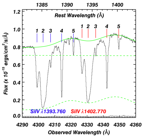
Figure 2: Intrinsic absorption troughs associated with Si iv in the VLT X-Shooter spectrum of SDSS J1512+1119. At the resolution of the instrument, the outflow is resolved in five unblended components spanning a range of velocities between -2100 and -520 km s^-1. The continuous line represents the unabsorbed emission model we built (see Section 3.1), and the dashed lines represents the continuum and emission line models.

Comparing the unblended line profile of the Si iv doublet, we distinguish five main kinematic components associated with the intrinsic outflow in our VLT X-Shooter data. The centroid of the absorption features are located at radial velocities $v\sim$ -2100, -1850, -1500, -1050, and -520 km s^-1 in the rest frame of SDSS J1512+1119 (see Figure 2). Using the Si iv components as a template, we identify absorption troughs associated with the kinematic components in a series of ions spanning a range of ionization. While the kinematic components are deep and blended together in the ubiquitous Ly$\alpha$, Ly$\beta$, O vi, N v and C iv transitions, some of the components are resolved in the Mg ii, C ii, Si ii, Si iii, Al ii, Al iii and He i* lines (see Figure 3). We report the detection of deep absorption troughs associated with the P v doublet in the component located at -1850 km s^-1 (component 2, see Figure 3), as well as absorption associated with ground state and excited S iv, and excited C iii and Fe iii. Of particular interest in this component is the detection of the high ionization excited S iv $\lambda$1073.51 transition, a line ten times weaker than the S iv $\lambda$1072.96 arising from the same excited level. The combined detection of these lines allows us to accurately determine the total S iv column density for that system (see Section 3.2). In the remainder of this analysis we will focus our attention on component 2, deferring the study of the other components to a forthcoming paper.

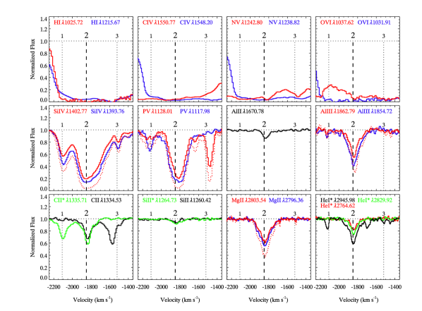
Figure 3: Normalized absorption line profiles of the absorption troughs associated with the UV outflow in SDSS J1512+1119 for kinematic component 2. For unblended doublets, we overplot the expected residual intensity in the strongest component based on the residual flux observed in the weakest component assuming the absorbing material completely and homogeneously covers the emission source ($I_{dotted}=I_{R}^{2}$, where $I_{R}$ is the residual intensity in the weaker component of the doublet).

3.1 Ionic column densities

In order to compute the column densities, we first need to estimate the spectrum of the background source (continuum and emission lines) illuminating the absorbing material. We model the unabsorbed and dereddened (E(B-V)=0.051 Schlegel et al. (1998)) continuum by a single power law of the form $F_{\lambda}=F_{1100}(\lambda/1100)^{\alpha}$, where $F_{1100}=77.01\pm 0.05\times 10^{17}$ erg/cm²/s/Å is the observed flux at 1100 Å (rest frame) and the power law index $\alpha=-0.403\pm 0.004$. Given the overall high S/N of the X-Shooter data (S/N $\sim$ 30 – 70 over most of the UVB/VIS range), we then fit the unabsorbed line emission using a smooth third order spline fit. We constrain the emission model over the broader troughs associated with Ly$\beta$, O vi, Ly$\alpha$, N v, and C iv by using the profiles derived from the unabsorbed red wings of each emission line. This fitting procedure is particularly effective given the tight constraints on the unabsorbed emission due to the high S/N and the presence of mainly narrow absorption features across the spectrum.

Once normalized by the emission profile, we extract the ionic column densities $N[$ion$]$ for each species by modeling the observed residual intensity $I_{i}$ (see Figure 3) inside the troughs as a function of the radial velocity. We use three different models in order to account for inhomogeneities in the absorbing material; apparent optical depth (AOD), partial covering (PC) and a power law model (PL) (see Edmonds et al., 2011; Borguet et al., 2012, for details). We integrate the line of sight averaged column density (Hamann & Sabra, 2004; Edmonds et al., 2011) over the radial velocity range $v\in[-2030,-1570]$ km s^-1 corresponding to kinematic component 2 and report the values in Table 1. We only report lower limits derived with the AOD model on column densities for singlet lines (Al ii, C ii, Si ii) as well as for deep/self-blended troughs such as O vi, C iv, and N v.

For photoionization modeling, actual $N[$ion$]$ measurements with robust error bars are much more useful than lower (or upper) limits. We now demonstrate that the troughs of Al iii, P v and He i* are not heavily saturated and therefore reliable $N[$ion$]$ measurements can be extracted for them. In Section 3.2 we show that this is also the case for S iv*. Let us first examine the Al iii, and P v doublets, where the oscillator strength $(f)$ of the blue transition is twice that of the red transition. From Figure 3 we can infer that in both cases the residual intensity of the red doublet component ($I_{r}$) is significantly higher than residual intensity of the blue doublet component ($I_{b}$) along essentially the entire absorption trough. Such a situation implies the true ionic column density in the trough cannot be much larger than 2-3 times that of an AOD estimate (see detailed treatment of this issue in Arav et al. 2005, 2008). Our Table 1 shows that this is indeed the case for Al iii, and P v, where we are able to measure robust $N[$ion$]$ for these ions using all three absorption models. If we define the saturation as $S\equiv N[$ion$]$(PL)/$N[$ion$]$(AOD) then the level of saturation in these troughs (from Table 1) is less than 1.2 for Al iii, and less than 3 for P v (even when taking the large upper error bar on the P v measurement). Similarly the He i* is even less saturated ($S<1.1$). Under these conditions, the exact behavior of the covering fraction as a function of velocity ($C(v)$) across the trough for the PC model, or that of the exponent $a(v)$ of the PL method, do not affect the robustness of the derived $N[$ion$]$.

While Si iv does not seem particularly saturated in Figure 3, we have to stress the fact that the normalization of the line profile was performed under the assumption that the absorbing material covers the emission sources (continuum and emission lines) by the same fraction. A closer inspection of the non-normalized O vi and C iv absorption troughs, however, reveal the existence of residual emission indicating that at least part of the emission lines (the intermediate/narrow emission component) are not fully covered by the absorber as observed in other outflows (e.g. Arav et al., 1999a; Gabel et al., 2006). Failure to account for this observation leads to an underestimation of the total Si iv column density since the weaker line emission under the blue absorption trough relative to the red would mislead the observer by making the doublet appear non-saturated (see Figure 2). For this reason, we report a lower limit on the Si iv column density in Table 1. Another transition that could be affected by this problem is Mg ii, although in this case, the weaker underlying line emission would only affect the absorption profile of the red component of the doublet. Other non-saturated species (P v, Al iii etc.) are located further away from significant emission lines in the SDSS J1512+1119 spectrum and are therefore not affected by this problem. In the last column of Table 1, we report the column densities used in the photoionization analysis. Those column densities are selected according to the following procedure: we use the values reported in the PC column as the measurements and the PL measurement and error as the upper error in order to account for possible inhomogeneities in the absorber (see Borguet et al., 2012). When only AOD determinations are available, we consider the reported values minus the error as a lower limit.

Table 1: Computed column densities

Ion	AODa	PCa	PLa	Adoptedb
	$10^{12}\mathrm{cm}^{-2}$	$10^{12}\mathrm{cm}^{-2}$	$10^{12}\mathrm{cm}^{-2}$	$10^{12}\mathrm{cm}^{-2}$
H i	$>765$	…		$>765$
He i*	687${}^{+22}_{-21}$	695${}^{+10}_{-10}$	715${}^{+27}_{-9}$	695${}^{+47}_{-10}$
C ii	214${}^{+4}_{-4}$	…		$>210$
C iv	$>2550$	…	…	$>2550$
N v	$>3280$	…	…	$>3280$
O vi	$>3940$	…	…	$>3940$
Mg ii	24.8${}^{+0.3}_{-0.3}$	35.6${}^{+0.6}_{-0.5}$	51.9${}^{+1.0}_{-1.0}$	35.6${}^{+17.3}_{-0.5}$
Al ii	1.76${}^{+0.08}_{-0.08}$	…		$>1.68$
Al iii	42.4${}^{+0.7}_{-0.7}$	51.0${}^{+0.8}_{-0.7}$	55.7${}^{+0.8}_{-0.7}$	51.0${}^{+5.5}_{-0.7}$
Si ii	4.05${}^{+0.37}_{-0.35}$	…	…	$>3.7$
Si iii	23.3${}^{+0.2}_{-0.2}$	…	…	$>23.1$
Si iv	391${}^{+2}_{-2}$	529${}^{+5}_{-4}$	$>800$	$>$525
P v	343${}^{+5}_{-5}$	444${}^{+13}_{-10}$	695${}^{+211}_{-8}$	444${}^{+462}_{-10}$
S ivc	…	….	…	26600${}^{+4000}_{-2700}$

a) The integrated column densities for the three absorber models. The quoted error arise from photon statistics only and are computed using the technique outlined in Gabel et al. (2005b).
b) Adopted values for the photoionization study (see text).
c) See Section 3.2 for details.

3.2 The S iv column density

The combined good S/N, medium resolution and moderate Ly forest contamination in the X-Shooter spectrum of SDSS J1512+1119 allow us to identify and separate the absorption troughs associated with S iv in kinematic component 2 of the outflow. As discussed in Leighly et al. (2009, 2011), S iv is composed of three lines; the ground state transition with a wavelength of 1062.66 Å, and two transitions arising from an excited state ($E=951$ cm^-1, referred to as S iv* in the following) at wavelengths 1072.96 and 1073.51 Å, the excited state being populated at a critical density of $4.7\times 10^{4}$ cm^-3. A useful feature of these lines is that the fractional abundance of S iv peaks at a similar ionization parameter to that of the ubiquitous C iv, implying that they arise in similar regions of the outflow (Dunn et al., 2012). The presence of two excited S iv* transitions with oscillator strengths an order of magnitude apart (Hibbert et al., 2002) provides sensitivity to a wide range of optical depths before both troughs become fully saturated.

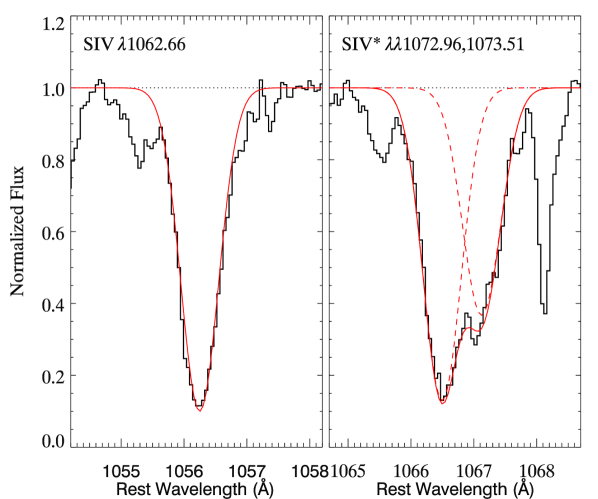
Figure 4: Result of the simultaneous fit (continuous smooth line) to the three S iv lines present in component 2. Within the uncertainties, the fitted profiles of the resonance $\lambda$1062.66 and excited $\lambda$1072.97 lines are identical, suggesting that the line profiles are saturated and no column density information can be derived from them. However, the detection of the excited 1073.51 Å line, a transition ten times weaker than the 1072.97 Å line, allows us to estimate the real S iv* column density.

In Figure 4, we present the result of the simultaneous Gaussian fit performed over the observed line profiles of the three S iv lines associated with component 2 of the outflow. The fit was performed by fixing the wavelength positions of the lines relative to the velocity of the component derived from the strong P v $\lambda 1117.98$ line profile as well as imposing an identical $FWHM$ for the three Gaussians, leaving only the depth of each component as a free parameter. The result of the fit clearly shows a detection of the weak excited $\lambda$1073.51 transition, translating to a high S iv* column density. Such a high column density leads to the conclusion that the $\lambda$1072.97 transition is optically thick and that the non-black profile observed is due to the partial covering of the emission source by the absorbing material. The depth of the resonance $\lambda$1062.66 line is consistent, within the uncertainties, with the depth derived from the $\lambda$1072.97 excited line implying that the $\lambda$1062.66 profile is also only reflecting a partial covering of the emission source. Note that the presence of a trough associated with component 1 of the outflow is observed in S iv around 1055.2 Å and in S iv* $\lambda$1072.97 around 1065.5 Å could affect the result of the fit if the optical depth in that system is large enough to produce a significant S iv* $\lambda$1073.51 trough. However, the high covering deduced from other high ionization lines (e.g. C iv, Si iv) for that component suggests a low optical depth ($\tau\simeq 0.2$) associated with the $\lambda$1072.97 translating to a $\tau\simeq 0.02$ for the ten times weaker $\lambda$1073.51 transition. Such a tiny optical depth will not affect the presented modeling of trough 2. Using the Gaussian model of the non-saturated $\lambda$1073.51 line profile along with the fact that the $\lambda$1072.97 line profile is saturated provides an unequivocal determination of the covering fraction across the trough (i.e. $C=1-I_{i}$ for saturated lines). We solve the PC model residual intensity equations for both S iv* transitions simultaneously and estimate the total S iv* column density to be $N[$S iv*$]\sim 1.6\times 10^{16}$ cm^-2.

In order to determine the total column density in S iv, we also have to be able to estimate the column density present in the ground state transition. As detailed above, the $\lambda$1062.66 line is saturated so that no accurate column density can be derived from the depth of the line profile. However, knowing the electron density $n_{e}$ of the gas would allow us to estimate the total S iv column density by comparing the measured value to models predicting the population ratio in the excited state to the ground state as a function of $n_{e}$. The detection of a blend of lines that we identify with the C iii* multiplet gives us the possibility to do so. As detailed in Gabel et al. (2005a), the excited C iii $\lambda$1175 multiplet comprises 6 lines arising from 3 J levels. The J=0 and J=2 levels have significantly lower radiative transition probabilities to the ground state than the J=1 level and are thus populated at much lower densities than the latter. In particular, Figure 5 in Gabel et al. (2005a) shows that the relative populations of the three levels are a sensitive probe to a wide range of $n_{e}$ while being insensitive to temperature. In Figure 5, we show several fits of the C iii* multiplet assuming a broadened Gaussian optical depth distribution for each line. The broadened Gaussian optical depth profile is identical for each line of the blend, only the optical depth varyies between the lines. The profile composed of a main central Gaussian profile (FWHM $=70$ km s^-1) containing the core of the optical depth ($\tau_{core}$) centered at the radial velocity identical to the centroid of the P v $\lambda 1117.98$ feature. Two weaker Gaussians ($\tau=0.2\tau_{core}$) with FWHM $=70$ km s^-1 are added at $\pm 70$ km s^-1 of the core Gaussian in order to produce the broadened wings. The fitting model is tightly constrained by the exact kinematic position (derived from the P v trough) and given the kinematic separation of the six C iii* components. The fit was repeated for various electron densities in the range $\log(n_{e})\in[3,10]$ with a step of 0.1 dex. The only free parameters for each model were a single optical depth and covering fraction. The best fit was found using a $\chi^{2}$ figure of merit for a density of $\log(n_{e})\sim 5.4$ cm^-3. We estimated conservative error-bars on the electron density by noting that for densities lower than $\log(n_{e})\raisebox{-2.15277pt}{$\;\stackrel{{\scriptstyle>}}{{\sim}}\;$}4.8$ the population of the J=2 level is too low to produce enough absorption (upper left panel of Figure 5) while the absence of significant contribution from J=1 lines limits the maximum density to $\log(n_{e})\raisebox{-2.15277pt}{$\;\stackrel{{\scriptstyle<}}{{\sim}}\;$}8.1$ (lower right panel of Figure 5). Electron number densities within the range $4.8\geq\log(n_{e})\geq 8.1$ provides acceptable fit to the blend. The density estimated from the C iii* fit is in good agreement with the detection of Fe iii* lines from the UV34 multiplet (see Borguet et al. 2012b, in preparation) which have a critical density of $\sim~{}10^{5}$ cm^-3 and with the absence of Fe iii* lines from the UV48 multiplet for which the critical density is $\sim~{}10^{10}$ cm^-3 (Bautista 2008, private communication). Assuming the electron density derived above and that the level population of S iv* relative to S iv are determined by collisional excitation and radiative de-excitation only, we are able to estimate the column density in the S iv ground state to be $1.06^{+0.40}_{-0.27}$ $10^{16}$ cm^-2, where the errors reflect the uncertainty on $n_{e}$.

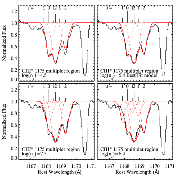
Figure 5: Fits to the normalized C iii* multiplet blend (continuous line) for component 2. The vertical lines plotted under each sub-component of the multiplet shows the location of the centroid of the line and the length of the mark indicates the relative oscillator strength of the line. The absorption line located at 1170.6 Å  is an unrelated line belonging to the Ly forest. We present the fit of the blended profile assuming the ratio between the J levels for four representative electron number densities. The lower limit on the possible $n_{e}$ is constrained by the inability of the model to fit the absorption associated with the longer wavelength J=2 transition (upper left). The upper limit on the $n_{e}$ range is fixed by the the apparition of significant absorption associated with the J=1 level for $\log(n_{e})\geq 8.1$ (lower right). The best fit of the blend is obtained for $\log(n_{e})=5.1$ (upper right panel). Other densities within the range $4.8\geq\log(n_{e})\geq 8.1$ lead to acceptable fits of the blend (lower left panel).

4 Photoionization modeling and relative abundance of phosphorus

4.1 Physical state of the gas assuming solar abundances

In this section we use the column densities determined for each of the ionic species to constrain the physical state (ionization parameter $U$, and total hydrogen column density $N_{H}$) of the gas. We model the absorber by a plane parallel slab of gas of constant hydrogen number density ($n_{H}$) and use the spectral synthesis code Cloudy C10.00 (last described in Ferland et al. 1998) to solve the ionization equilibrium equations. We assume solar abundances for the gas from Lodders et al. (2009). Due to the lack of constraints on the EUV/FUV region of the spectral energy distribution (SED) of SDSS J1512+1119, we adopt the “UV-soft” SED proposed for luminous, Radio Quiet quasars in Dunn et al. (2010); their Figure 11. The features of this SED, which is discussed in detail in Dunn et al. (2010), departs from the “classical” Mathews & Ferland (1987) SED (MF87) by excluding the so called UV-bump peaking at FUV energies while keeping an $\alpha_{ox}$ index similar to that of MF87.

We use the grid model approach described in Edmonds et al. (2011) in order to determine the pair of parameters ($U$,$N_{H}$) that best reproduces the observed ionic column densities. We only consider column densities determined from non-saturated troughs, since the lower limits placed on the column densities from H i, C iv, N v, O vi are clear underestimations of their true values (see Section 3.1) and are consistent with the solution derived from the non-saturated lines. We have constraints from 10 ionic species : He i*, C ii, Mg ii, Al ii, Al iii, Si ii, Si iii, Si iv, P v and S iv. From this set, P v, S iv, He i* and Al iii are the most reliable as their $N[$ion$]$ is derived from two or more troughs that are not heavily saturated (see Section 3.1).

Given that the derived density of the absorbing material is well over the C ii critical density we conclude that our estimation of the C ii column density is robust within a factor of two, since for such a high density, the apparent strength of C ii* $\lambda 1335.71$ is approximately twice that of C ii $\lambda 1334.53$, allowing us to derive a PC and PL solution by applying a similar treatment to these lines as to resonance doublets. The other lines are either singlets for which a robust $N[$ion$]$ is difficult to ascertain in principle, or doublets that may be more heavily saturated (Si iv, Mg ii, see Section 3.1). We finally place an upper limit on the column density of the non-detected Fe ii by scaling the Mg ii blue line profile template to the $2\sigma$ noise in the region where the strongest Fe ii $\lambda$2382.77 should be located and find $N[$Fe ii$]<1.96\times 10^{12}$ cm^-2.

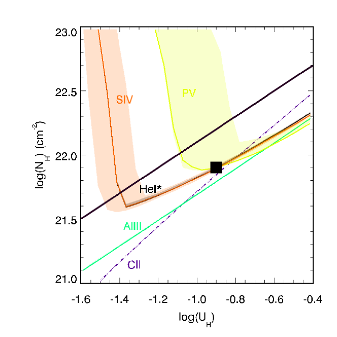
Figure 6: Grid model plot of the photoionization modeling of the absorber. Solid lines are the adopted $N[$ion$]$ measurements from Table 1. The shaded area represent the measured column density of the ion and its errors on these measurements due to the photon noise and the systematic uncertainties in the absorber model. Dotted-dashed line represent a lower limit on the column density. The black square represents the $U$ and $N_{H}$ that best reproduces the observed column densities (see text). The upper part of the phase plot (beyond the hydrogen ionization front characterized by $\log(N_{H})=23.1~{}\log(U)$) is an artifact of our modeling procedure. By coincidence the He i* and S iv lines almost track each other between $\log(U)=-1.4$ and $\log(U)=-0.5$. We represent the hydrogen ionization front ($\log(N_{H})=23.1\log(U_{H})$) by a thick black line.

Table 2: Photoionization model of the absorber

Ion	log($N_{obs}$) (cm-2)	log($N_{mod}$) (cm-2)	log$\left(\frac{N_{mod}}{N_{obs}}\right)$
	Adopted a	Cloudy
log $(U)$	$\cdots$	-0.90b
log $(N_{H})$	$\cdots$	21.9b
H i	$>14.88$	17.51	2.63
He i*	$14.84^{+0.03}_{-0.01}$	14.86	0.02
C ii	$\sim 14.33$	14.50	0.19
C iv	$>15.41$	17.91	2.50
N v	$>15.52$	16.91	1.40
O vi	$>15.60$	17.81	2.21
Mg ii	$13.55^{+0.17}_{-0.01}$	14.34	0.79
Al ii	$>12.23$	12.45	0.22
Al iii	$13.71^{+0.05}_{-0.01}$	14.13	0.42
Si ii	$>12.57$	12.96	0.39
Si iii	$>13.36$	15.09	1.73
Si iv	$>14.71$	16.24	1.52
P v	$14.65^{+0.31}_{-0.01}$	14.65	0.00
S iv	$16.43^{+0.06}_{-0.04}$	16.45	0.02

a) Adopted column densities reported in Table 1. Ions with robust measurements are marked in boldface.
b) Best fit Cloudy model.

We present the results for a grid of photoionization models in Figure 6. Visual inspection of the figure shows that a minimum ionization parameter of $\log(U)>-1.1$ is required by the P v constraints. The presence of the low ionization C ii, Si ii, and Al ii requires $\log(U)<-0.6$: although these low ionization species can also be formed at higher $U$ near a hydrogen ionization front in the absorber, such a model would overpredict well constrained ions like S iv or P v by a factor $\geq 5$. The corresponding total hydrogen column density is rather large due to the detection of P v as well as the high column density derived from the detailed analysis of the S iv troughs and suggests a thick absorber with $\log(N_{H})\in[21.5,21.9]$ for the range of ionization parameters considered here. Such a high column density is also supported by the detection of He i*, which implies an absorber with a thickness reaching well into the He ii region, while the clear non-detection of the strongest Fe ii lines implies the absence of the formation of a hydrogen ionization front in the slab. We determine the best ($U,N_{H}$) model by $\chi^{2}$ minimization of the difference between the measured column densities and those predicted by Cloudy (see Borguet et al., 2012) and find $\log(U)=-0.9$ and $\log(N_{H})=21.9$. In Table 2, we compare the measured column densities to those predicted by the best-fit model. Taking the uncertainties into account, the column densities associated with the ions for which we have a robust measurement are matched well within a factor of 2 while the Al iii column density is reproduced within a factor of 3. The computation shows also an underestimation by factors of hundreds for the usual high ionization lines, underlining the fact that AOD measurements yield a poor estimate of the actual column densities for these species.

4.2 Constraining the relative phosphorus abundance

In this section, we use our knowledge of the photoionization solution and the measurements of the column densities of P v and mainly He i* in order to constrain the abundance of phosphorus in the outflowing material. Let us first assume that all elements except phosphorus have solar abundances. Given the photoionization solution determined in Section 4.1, the abundance of phosphorus relative to helium is constrained by the upper-limit on the column density of P v to be $\raisebox{-2.15277pt}{$\;\stackrel{{\scriptstyle<}}{{\sim}}\;$}2$ times the solar value. In these models, we use a hydrogen number density of $10^{4}$ cm^-3, which is close to the lower limit determined in Section 3.2. Increasing the hydrogen number density to $10^{8}$ cm^-3, the upper limit on the number density, increases $U$ and $N_{H}$ by 0.1 dex each and reduces the upper limit on the abundance ratio P/P_⊙. We therefore conclude that, for solar abundances of the other elements, the phosphorus abundance is approximately solar.

While the parameter fit using solar abundances is very good, we consider the effects of changing metalicity on the phosphorus abundance. For our purposes, we consider a gas with metalicity Z/Z_⊙ = 1 to have solar abundances, noting that the scaling of heavy elements with Z is model dependent (e.g. Hamann & Ferland, 1993; Korista et al., 1996). Figure 7 is a grid model plot for photoionization models with Z/Z${}_{\odot}\approx 4$. We use the abundance scalings provided in Table 2 of Ballero et al. (2008) for C, N, O, Mg, Si, Ca, and Fe. Scalings for the other metals as well as helium are estimated using starburst models in Cloudy for Z/Z_⊙ = 4. For these models, any solution that reasonably reproduces column densities of the metals underestimates the column density of helium by a factor $\sim 2$ for a number density of $10^{4}$ cm^-3 and less than a factor of 2 for a number density of $10^{8}$ cm^-3 . Increasing the metalicity increases this discrepancy, thus we conclude that Z/Z${}_{\odot}\raisebox{-2.15277pt}{$\;\stackrel{{\scriptstyle<}}{{\sim}}\;$}4$. We find that none of the models accurately reproduce our measured ionic column densities if the metal abundances are reduced by a factor $\sim 2$, implying that the gas is has a metalicity Z/Z${}_{\odot}\raisebox{-2.15277pt}{$\;\stackrel{{\scriptstyle>}}{{\sim}}\;$}0.5$. Constraining the metalicity to 0.5$\leq$Z/Z${}_{\odot}<$4 limits the ionization parameter to $-1.3\raisebox{-2.15277pt}{$\;\stackrel{{\scriptstyle<}}{{\sim}}\;$}U\raisebox{-2.15277pt}{$\;\stackrel{{\scriptstyle<}}{{\sim}}\;$}-0.5$. Comparing phosphorus only to helium, we find that $1/2<$P/P${}_{\odot}<5$. The upper limit is overly conservative and is the maximum over-abundance of phosphorus that allows the models to produce enough He i*.

Ionization and thermal structures in the absorber depend on the SED incident on the outflowing gas. In the foregoing analysis, we used the UV-soft SED mentioned in Section 4.1. We tested several SEDs appropriate for radio-quiet quasars to determine their impact on our main results. The largest changes occurred for SEDs including a substantial “UV bump”. In particular, using MF87, we find the best fit model with solar abundances yields log $U=-1.1$ and log $N_{H}=21.6$. However, more importantly for our purposes here, our diagnostic line ratios change by factors $\raisebox{-2.15277pt}{$\;\stackrel{{\scriptstyle<}}{{\sim}}\;$}2$ for corresponding models. The major change is that the conservative upper limit on P/P_⊙ can be as large as 6 for the MF87 SED. However, we emphasize again that the MF87 SED is not a good approximation to a high luminosity radio quiet quasar.

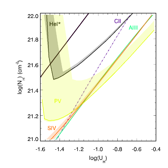
Figure 7: Identical to Figure 6 but assuming a metalicity of $Z=4$ (see Section 4.2 for details). It is clear that no $U$ and $N_{H}$ solution can simultaneously satisfy the S iv and He i* measurements, as these curves never intersects.

4.3 The true C iv optical depth

For outflows that show a significant P v trough, our investigation gives us a unique empirical opportunity to contrast the apparent and real optical depth of the C iv trough arising from the same outflow. As can be seen in Figure 3, the residual intensity of the C iv trough in the deepest part of component 2 is $I_{i}\sim 0.025$, which yields an apparent optical depth of $\ln(I_{i})\sim 4$. The real optical depth of C iv at that velocity can be estimated using our derived photoionization parameters for the absorber along with the knowledge of the column density and abundance of an unsaturated line like P v. Assuming solar abundances for simplicity (the abundance of phosphorus does not deviate widely from solar, see Section 4.2) we represent in Figure 8 the expected column density ratio $\log(N[$P v$]/N[$C iv$])$ as a function of $U$ and $N_{H}$. Using the ionization parameter of $\log(U)=-0.9$ and total hydrogen column density of $\log(N_{H})=21.9$ found in Section 4.1 we find $\log(N[$P v$]/N[$C iv$])\sim-3.3$. The ratio of optical depth for the two transitions is then given by:

$$\frac{\tau[\mathrm{C}\textsc{iv}]}{\tau[\mathrm{P}\textsc{v}]}=\frac{N[\mathrm{C}\textsc{iv}]}{N[\mathrm{P}\textsc{v}]}\frac{(f\lambda)_{\mathrm{C}\small{\textsc{iv}}}}{(f\lambda)_{\mathrm{P}\small{\textsc{v}}}}=10^{3.3}\frac{0.19}{0.45}\frac{1548.20}{1117.98}\sim 1200,$$ (1)

where $f$ is the oscillator strength and $\lambda$ is the wavelength of the given transition. Using the partial covering method on the P v doublet troughs we obtain a real optical depth for P v$\lambda$1117.98 of 2.7. Therefore, equation (1) yields a real C iv$\lambda$1548.20 optical depth of $\sim$3200! Or a value almost 1000 times larger than the apparent optical depth of C iv($\sim 4$). Thus the detection of P v troughs will indeed result in heavily saturated C iv line profiles, with a real optical depth roughly a thousand times higher than the apparent one.

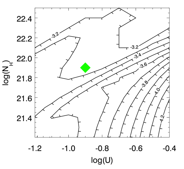
Figure 8: This plot shows contours of the logarithm of the predicted ratio of column density between P v and C iv, $\log(N[$P v$]/N[$C iv$])$, as a function of the ionization parameter $U$ and the total hydrogen column density of the absorber $N_{H}$. Assuming solar abundances and the photionization solution found in Section 4.1 (represented by a solid diamond), Cloudy models predicts a ratio of column density of $\log(N[$P v$]/N[$C iv$])\sim-3.3$.

5 Summary

In this paper, we studied the UV outflow associated with the quasar SDSS J1512+1119 on the basis of new, medium resolution VLT/X-Shooter data. The extended wavelength coverage of the instrument allowed us to detect the outflow components in a multitude of ionic species. In particular we report the detection of deep P v absorption troughs in kinematic component 2 as well as the detection of S iv and S iv*. A detailed analysis of the S iv* line profile allowed us to detect the weak $\lambda 1073.51$ transition revealing a S iv column density larger than suggested by the apparent depth of the absorption troughs of the $\lambda 1072.97$ transition.

Photoionization modeling of the absorber revealed that the absorber is thick, though the non-detection of significant Fe ii absorption troughs guarantees the absence of a significant amount of H i bound-free opacity. Our accurate determination of the total P v  S iv  He i* and lower ionization species column densities allowed us to characterize the physical state of the gas. We find that for the range of ionization parameters relevant for the present absorber, the phosphorus abundance relative to helium is consistent with the solar value. Using the parameter derived from the photoionization analysis, we show, as suggested in Hamann (1998), that a line such as the ubiquitous C iv is heavily saturated. The C iv column density derived from the apparent depth of the absorption line profile underestimates the column density by a factor of $\sim$1000, providing a very poor estimate of its true column density.

The phosphorus abundance we find is in disagreement with the extreme phosphorus abundances reported in the early literature (e.g. Junkkarinen et al., 1995, 1997; Hamann, 1998). Other elemental abundances are found to be in agreement with the solar values. The fact that the abundances are similar to the solar values for an odd (P v) and even (S iv) element points to enrichment by relatively “normal” galactic stellar populations (e.g. Hamann, 1997) rather than the more exotic mechanism proposed by Shields (1996) that would significantly enhance the P/S ratio (Hamann, 1998).

References

- Arav (1997) Arav, N. 1997, in Astronomical Society of the Pacific Conference Series, Vol. 128, Mass Ejection from Active Galactic Nuclei, ed. N. Arav, I. Shlosman, & R. J. Weymann, 208
- Arav et al. (1999a) Arav, N., Becker, R. H., Laurent-Muehleisen, S. A., Gregg, M. D., White, R. L., Brotherton, M. S., & de Kool, M. 1999a, ApJ, 524, 566
- Arav et al. (2001a) Arav, N., Brotherton, M. S., Becker, R. H., Gregg, M. D., White, R. L., Price, T., & Hack, W. 2001a, ApJ, 546, 140
- Arav et al. (2005) Arav, N., Kaastra, J., Kriss, G. A., Korista, K. T., Gabel, J., & Proga, D. 2005, ApJ, 620, 665
- Arav et al. (2003) Arav, N., Kaastra, J., Steenbrugge, K., Brinkman, B., Edelson, R., Korista, K. T., & de Kool, M. 2003, ApJ, 590, 174
- Arav et al. (2002) Arav, N., Korista, K. T., & de Kool, M. 2002, ApJ, 566, 699
- Arav et al. (1999b) Arav, N., Korista, K. T., de Kool, M., Junkkarinen, V. T., & Begelman, M. C. 1999b, ApJ, 516, 27
- Arav et al. (2008) Arav, N., Moe, M., Costantini, E., Korista, K. T., Benn, C., & Ellison, S. 2008, ApJ, 681, 954
- Arav et al. (2001b) Arav, N., et al. 2001b, ApJ, 561, 118
- Arav et al. (2007) —. 2007, ApJ, 658, 829
- Ballero et al. (2008) Ballero, S. K., Matteucci, F., Ciotti, L., Calura, F., & Padovani, P. 2008, A&A, 478, 335
- Ballester et al. (2011) Ballester, P., Bramich, D., Forchi, V., Freudling, W., Garcia-Dabó, C. E., klein Gebbinck, M., Modigliani, A., & Romaniello, M. 2011, in Astronomical Society of the Pacific Conference Series, Vol. 442, Astronomical Data Analysis Software and Systems XX, ed. I. N. Evans, A. Accomazzi, D. J. Mink, & A. H. Rots, 261
- Barai et al. (2011) Barai, P., Martel, H., & Germain, J. 2011, ApJ, 727, 54
- Barlow & Sargent (1997) Barlow, T. A., & Sargent, W. L. W. 1997, AJ, 113, 136
- Borguet et al. (2012) Borguet, B. C. J., Edmonds, D., Arav, N., Dunn, J., & Kriss, G. A. 2012, ApJ, 751, 107
- Churchill et al. (1999) Churchill, C. W., Mellon, R. R., Charlton, J. C., Jannuzi, B. T., Kirhakos, S., Steidel, C. C., & Schneider, D. P. 1999, ApJ, 519, L43
- Crenshaw et al. (2003) Crenshaw, D. M., Kraemer, S. B., & George, I. M. 2003, ARA&A, 41, 117
- Dai et al. (2008) Dai, X., Shankar, F., & Sivakoff, G. R. 2008, ApJ, 672, 108
- de Kool et al. (2001) de Kool, M., Arav, N., Becker, R. H., Gregg, M. D., White, R. L., Laurent-Muehleisen, S. A., Price, T., & Korista, K. T. 2001, ApJ, 548, 609
- Di Matteo et al. (2004) Di Matteo, T., Croft, R. A. C., Springel, V., & Hernquist, L. 2004, ApJ, 610, 80
- Dietrich et al. (2003) Dietrich, M., Appenzeller, I., Hamann, F., Heidt, J., Jäger, K., Vestergaard, M., & Wagner, S. J. 2003, A&A, 398, 891
- Dunn et al. (2012) Dunn, J. P., Arav, N., Aoki, K., Wilkins, A., Laughlin, C., Edmonds, D., & Bautista, M. 2012, ApJ, 750, 143
- Dunn et al. (2008) Dunn, J. P., Crenshaw, D. M., Kraemer, S. B., & Trippe, M. L. 2008, AJ, 136, 1201
- Dunn et al. (2010) Dunn, J. P., et al. 2010, ApJ, 709, 611
- Edmonds et al. (2011) Edmonds, D., et al. 2011, ApJ, 739, 7
- Elvis (2006) Elvis, M. 2006, Mem. Soc. Astron. Italiana, 77, 573
- Ferland et al. (1998) Ferland, G. J., Korista, K. T., Verner, D. A., Ferguson, J. W., Kingdon, J. B., & Verner, E. M. 1998, PASP, 110, 761
- Gabel et al. (2006) Gabel, J. R., Arav, N., & Kim, T. 2006, ApJ, 646, 742
- Gabel et al. (2005a) Gabel, J. R., et al. 2005a, ApJ, 631, 741
- Gabel et al. (2005b) —. 2005b, ApJ, 623, 85
- Ganguly et al. (1999) Ganguly, R., Eracleous, M., Charlton, J. C., & Churchill, C. W. 1999, AJ, 117, 2594
- Germain et al. (2009) Germain, J., Barai, P., & Martel, H. 2009, ApJ, 704, 1002
- Hamann (1997) Hamann, F. 1997, ApJS, 109, 279
- Hamann (1998) —. 1998, ApJ, 500, 798
- Hamann et al. (1997) Hamann, F., Barlow, T. A., Junkkarinen, V., & Burbidge, E. M. 1997, ApJ, 478, 80
- Hamann & Ferland (1993) Hamann, F., & Ferland, G. 1993, ApJ, 418, 11
- Hamann & Ferland (1999) —. 1999, ARA&A, 37, 487
- Hamann et al. (2002) Hamann, F., Korista, K. T., Ferland, G. J., Warner, C., & Baldwin, J. 2002, ApJ, 564, 592
- Hamann & Sabra (2004) Hamann, F., & Sabra, B. 2004, in Astronomical Society of the Pacific Conference Series, Vol. 311, AGN Physics with the Sloan Digital Sky Survey, ed. G. T. Richards & P. B. Hall, 203
- Hamann et al. (2003) Hamann, F., Sabra, B., Junkkarinen, V., Cohen, R., & Shields, G. 2003, ArXiv Astrophysics e-prints
- Hamann et al. (2007) Hamann, F., Warner, C., Dietrich, M., & Ferland, G. 2007, in Astronomical Society of the Pacific Conference Series, Vol. 373, The Central Engine of Active Galactic Nuclei, ed. L. C. Ho & J.-W. Wang, 653
- Hewett & Foltz (2003) Hewett, P. C., & Foltz, C. B. 2003, AJ, 125, 1784
- Hewett & Wild (2010) Hewett, P. C., & Wild, V. 2010, MNRAS, 405, 2302
- Hibbert et al. (2002) Hibbert, A., Brage, T., & Fleming, J. 2002, MNRAS, 333, 885
- Horne (1986) Horne, K. 1986, PASP, 98, 609
- Juarez et al. (2009) Juarez, Y., Maiolino, R., Mujica, R., Pedani, M., Marinoni, S., Nagao, T., Marconi, A., & Oliva, E. 2009, A&A, 494, L25
- Junkkarinen et al. (1997) Junkkarinen, V., Beaver, E. A., Burbidge, E. M., Cohen, R. D., Hamann, F., & Lyons, R. W. 1997, in Astronomical Society of the Pacific Conference Series, Vol. 128, Mass Ejection from Active Galactic Nuclei, ed. N. Arav, I. Shlosman, & R. J. Weymann, 220
- Junkkarinen et al. (1995) Junkkarinen, V. T., Beaver, E. A., Burbidge, E. M., Cohen, R. D., Hamann, F., Lyons, R. W., & Barlow, T. A. 1995, in Bulletin of the American Astronomical Society, Vol. 27, American Astronomical Society Meeting Abstracts #186, 872
- Knigge et al. (2008) Knigge, C., Scaringi, S., Goad, M. R., & Cottis, C. E. 2008, MNRAS, 386, 1426
- Korista et al. (1996) Korista, K., Hamann, F., Ferguson, J., & Ferland, G. 1996, ApJ, 461, 641
- Leighly et al. (2011) Leighly, K. M., Dietrich, M., & Barber, S. 2011, ApJ, 728, 94
- Leighly et al. (2009) Leighly, K. M., Hamann, F., Casebeer, D. A., & Grupe, D. 2009, ApJ, 701, 176
- Lodders et al. (2009) Lodders, K., Palme, H., & Gail, H.-P. 2009, in ”Landolt-Börnstein - Group VI Astronomy and Astrophysics Numerical Data and Functional Relationships in Science and Technology Volume, ed. J. E. Trümper, 44
- Mathews & Ferland (1987) Mathews, W. G., & Ferland, G. J. 1987, ApJ, 323, 456
- Modigliani et al. (2010) Modigliani, A., et al. 2010, in Society of Photo-Optical Instrumentation Engineers (SPIE) Conference Series, Vol. 7737, Society of Photo-Optical Instrumentation Engineers (SPIE) Conference Series
- Moe et al. (2009) Moe, M., Arav, N., Bautista, M. A., & Korista, K. T. 2009, ApJ, 706, 525
- Ostriker et al. (2010) Ostriker, J. P., Choi, E., Ciotti, L., Novak, G. S., & Proga, D. 2010, ApJ, 722, 642
- Sargent et al. (1988) Sargent, W. L. W., Boksenberg, A., & Steidel, C. C. 1988, ApJS, 68, 539
- Schlegel et al. (1998) Schlegel, D. J., Finkbeiner, D. P., & Davis, M. 1998, ApJ, 500, 525
- Scott et al. (2004) Scott, J. E., et al. 2004, ApJS, 152, 1
- Shields (1996) Shields, G. A. 1996, ApJ, 461, L9
- Telfer et al. (1998) Telfer, R. C., Kriss, G. A., Zheng, W., Davidsen, A. F., & Green, R. F. 1998, ApJ, 509, 132
- Turnshek (1986) Turnshek, D. A. 1986, in IAU Symposium, Vol. 119, Quasars, ed. G. Swarup & V. K. Kapahi, 317–328
- Turnshek et al. (1996) Turnshek, D. A., Kopko, Jr., M., Monier, E., Noll, D., Espey, B. R., & Weymann, R. J. 1996, ApJ, 463, 110
- Vernet et al. (2011) Vernet, J., Dekker, H., D’Odorico, S., Kaper, L., Kjaergaard, P., & Hammer, F. 2011, A&A, 536, A105