UV Properties of Galactic Globular Clusters with GALEX II. Integrated colors.

Abstract

We present ultraviolet (UV) integrated colors of 44 Galactic globular clusters (GGCs) observed with the Galaxy Evolution Explorer (GALEX) in both $FUV$ and $NUV$ bands. This data-base is the largest homogeneous catalog of UV colors ever published for stellar systems in our Galaxy. The proximity of GGCs makes it possible to resolve many individual stars even with the somewhat low spatial resolution of GALEX. This allows us to determine how the integrated UV colors are driven by hot stellar populations, primarily horizontal branch stars and their progeny. The UV colors are found to be correlated with various parameters commonly used to define the horizontal branch morphology. We also investigate how the UV colors vary with parameters like metallicity, age, helium abundance and concentration. We find for the first time that GCs associated with the Sagittarius dwarf galaxy have $(FUV-V)$ colors systematically redder than GGCs with the same metallicity. Finally, we speculate about the presence of an interesting trend, suggesting that the UV color of GCs may be correlated with the mass of the host galaxy, in the sense that more massive galaxies possess bluer clusters.

1 INTRODUCTION

The main contributors to the UV emission from any stellar system are the hottest stars. Indeed blue horizontal branch (HB) stars are well known to be among the hottest stellar populations in globular clusters (GCs) and contribute substantially to the UV radiation observed from old stellar systems (Welch & Code, 1972). Later on, two other sub-classes of post-HB stars were found to be important contributors to far-UV ($FUV$, $\lambda\sim 1500$–1600 Å) radiation (e.g., Greggio and Renzini 1990; Dorman et al. 1995, hereafter DOR95; Han et al. 2007). The hottest HB stars (extreme HB, EHB) have such a small envelope mass that most of their post-He-core burning phase takes place at high effective temperature ($T_{\rm eff}$), during the so called ”AGB-manqué phase”, and these stars never return to the asymptotic giant branch (AGB). Another group of UV-bright stars is that of post-early AGB stars, which after a brief return to the AGB, spend the bulk of their helium shell burning phase at high $T_{\rm eff}$. In systems with only red HB a small floor level of $FUV$ is provided by post-AGB stars, which evolve to the AGB phase with an higher envelope mass where they undergo thermal pulses and eventually lose their envelopes moving at higher temperatures at constant luminosity. The relative contributions of the various types of stars and the factors that might lead to larger or smaller populations of UV-bright stars have remained an open question (Greggio and Renzini 1990; DOR95; Lee et al. 2002; Rich et al. 2005; Sohn et al. 2006).

In distant extragalactic systems one can ordinarily observe only the integrated light of unresolved stellar populations, from which the hope is to gain knowledge about the underlying stellar population. Galactic globular clusters (GGCs) play an important role in understanding the integrated UV colors of extragalactic systems, especially the so called ”UV-upturn” observed in the spectral energy distributions of elliptical galaxies (Code & Welch 1979; de Boer 1982; Bertola et al. 1982; Greggio & Renzini 1990; O’Connell 1999). First of all, GCs are the closest example in nature to a single stellar population (SSP): a system of coeval stars with similar chemical composition. Moreover GGCs span a large range of metallicities, a small range of ages, and perhaps some range of helium abundance. Hence they can be used to test the stellar evolution theory, which in turn is one of the basic ingredients of the models used to interpret the integrated light of distant galaxies. GGCs are relatively nearby objects (more than $\sim 90\%$ are located at distances $r<30$ kpc), so their populations can be easily resolved. With typically more than 100,000 stars, even relatively short-lived evolutionary stages are sampled. We can directly observe the properties of individual stars and measure the population ratios for objects in different evolutionary stages. In particular we can study the impact of hot and bright populations (as the AGB-manqué stars) on the integrated UV light of GGCs and then use them as crucial local templates for comparison with integrated properties of distant extragalactic systems. In fact comparing features in the color-magnitude diagrams (CMDs) of well known and resolved GGCs with integrated quantities can lend important model independent insights into the nature of extragalactic systems.

Integrated UV photometry of GGCs has previously been obtained by the Orbiting Astronomical Observatory (OAO 2; Welch & Code 1980), Astronomical Netherlands Satellite (ANS; van Albada, de Boer & Dickens 1981), Ultraviolet Imaging Telescope (UIT; Hill et al. 1992; Landsman et al. 1992; Parise et al. 1994; Whitney et al. 1994), and International Ultraviolet Explorer (IUE; Castellani & Cassatella 1987). Using a large, but heterogeneous, collection of data obtained with some of these telescopes along with population synthesis models, DOR95 showed how the UV colors varied with parameters like metallicity and how they compare with elliptical galaxies. They showed how the UV colors of GGCs could plausibly be produced by hot HB stars and their progeny.

At the time of DOR95, UV photometry of individual stars in GGCs was available for only a few clusters. That situation has changed dramatically. Our group alone has already published HST UV photometry for a dozen of GGCs (see Ferraro et al. 1997, Ferraro et al. 1998, Ferraro et al. 1999, Ferraro et al. 2001, Ferraro et al. 2003, Lanzoni et al. 2007, Dalessandro et al. 2008, Rood et al. 2008) and obtained data for an additional 32 clusters in HST Cycle 16S (GO11975, PI: Ferraro; see Contreras et al. 2012, Sanna et al. 2012 and references therein).

More recently, we have secured observations of 44 GGCs during three observing cycles with the Galaxy Evolution Explorer (GALEX). This is the largest homogeneous sample ever collected for GGCs in UV so far. In Schiavon et al. (2012; hereafter Paper I) we presented photometry and CMDs for these clusters. Here we present integrated UV magnitudes and colors (§ 2) for each cluster, and we describe (§ 3) how they are affected by HB class, metallicity, age, and possibly structural parameters (mass, density, central relaxation time, etc.). In § 4 we compare our data with observations of GCs in M31 and M87.

2 OBSERVATIONS and DATA ANALYSIS

Images for 38 GGCs were obtained as part of GI1 and GI4 GALEX programs (P.I. R. P. Schiavon) and supplemented with somewhat shallower exposures for 8 GGCs obtained as part of program GI3 (P.I., S. Sohn). Two clusters (NGC 6229 and NGC 6864) are in common between the two programs. A number of clusters that would have been very interesting targets (including M13, M80, $\omega$ Centauri, NGC 6388, and NGC 6441) could not be observed because of restrictions on the UV background brightness, due to detector-safety considerations, which prevented us from targeting at low Galactic latitudes, or near positions of very bright UV sources. With only one exception (NGC 6273), images were obtained in both the $FUV$ ($\lambda_{c}=1516$ Å) and near-UV ($NUV$, $\lambda_{c}=2267$ Å) bands. Thanks to the wide field of view of GALEX ($\sim 1.2\deg$), it has been possible to sample the full radial extent of most of the clusters. A few GCs, like NGC 104 (47Tuc) and NGC 5272 (M3), have tidal radii larger than the GALEX field of view (McLauglhin & van der Marel 2005, hereafter MVM05), but these missing data do not significantly affect our analysis. Each GALEX image has been pre-processed by the standard pipeline described in detail by Morrissey et al. (2005). The raw images (or “count images”) have been converted to flux-calibrated intensity images by applying relative response and flat-field corrections and by scaling the flux by the effective area and exposure time.

3 INTEGRATED MAGNITUDES

The integrated magnitudes have been obtained using two different approaches: (i) by fitting the surface brightness profiles (SBPs), and (ii) from direct aperture photometry (AP) measurement on the images. In both approaches, the integrated photometry will include the effects of objects below the detection threshold for individual stars. Comparing the results obtained with these two different approaches we can correct for systematic effects or biases. In particular, AP can be affected by small number statistics when a few very bright stars dominate the flux, especially at $FUV$ wavelengths (as for example, the case of the bright star in the very central regions of 47 Tuc reported by O’Connell et al. 1997). These very bright objects may be cluster members (post-HB or post-AGB star) or just foreground stars. On the other hand, while colors obtained by the SBP method are less affected by star count fluctuations, they may suffer from uncertainties arising from the quality of the fit or the determination of the center of the cluster. For these reasons we have calculated integrated magnitudes with both the techniques, and we have compared the results in detail.

In both cases, it was first necessary to determine the cluster centers. Since previous determinations (e.g., Harris 1996, 2010 revision – hereafter H10; Noyola & Gebhardt 2006; Goldsbury et al. 2010) either were obtained with quite heterogeneous methods, or only partially overlap our sample, we preferred to perform new estimates. The plate scale of GALEX ($1.5\arcsec\,{\rm pixel}^{-1}$ ) and the “noise” due to the relatively small number of stars detected at UV band introduce considerable uncertainty in the measurement of the barycenter of resolved stars (e.g., Lanzoni et al. 2007). We therefore determined the center of the light distribution on $NUV$ images by following the same approach described in Bellazzini (2007). For any given GC we picked an aperture radius that, based on the size of cluster central region and its density, was large enough to include a good fraction of the brightest sources. We then determined the light density (i.e. the fraction of observed flux per unit area) in that aperture and iteratively varied the centering position until maximum light density was found. We do not list the centers of light, since they have been obtained in instrumental coordinates and therefore they could be used only when the images they refer to are available. Moreover the poor spatial resolution of the GALEX detectors would have prevented to obtain a sufficient level of accuracy to make these values useful to the community for other applications.

3.1 Integrated magnitudes from surface brightness profile fitting

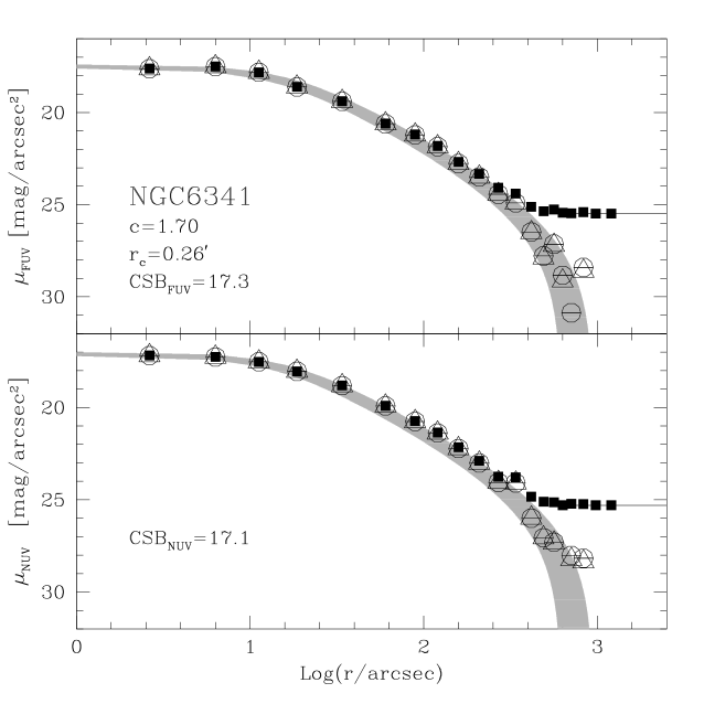
Figure 1: $FUV$ and $NUV$ surface brightness profiles for NGC 6341. The black squares represent the observed raw profile, while open circles are the sky-subtracted values. The horizontal black lines mark the estimated background level. The background-subtracted profiles obtained by using standard IRAF routines are shown with open triangles, for comparison (see Section 3.1 for details). The profiles are well reproduced by the King model (the grey region is defined by the structural parameters uncertainties) with concentration parameter and core radius quoted by MVM05 and with central surface brightness (CSB) value providing the minimum $\chi^{2}$ (see labels).

SBPs were obtained by using concentric annuli centered on the cluster centers determined as described above. The number and the size of the annuli were chosen for each cluster so as they sampled almost the same light fraction. The flux calculation was performed by using standard IRAF tasks (PHOT, in the DAOPHOT package, Stetson 1987). The flux calculated in each annulus was normalized to the sampled area obtained adopting as pixel size $1.5\arcsec$, as reported by Morrissey et al. (2005) for intensity map images. The instrumental surface brightness profiles were then transformed to the ABMAG GALEX magnitude system by applying the zero-points reported in the GALEX on-line user’s manual or in Section 4.2 of Morrissey et al. (2005). As an example, the observed SBP of NGC 6341 is shown in Figure 1 for both the $FUV$ and $NUV$ channels. In this figure, solid squares are the annular surface brightness measurements at each cluster radius, whereas open circles represent the same values after performing sky subtraction as described below.

Using SBPs to obtain integrated colors requires the subtraction of the background contribution, which is the combination of the sky background emission (due to unresolved objects) and the resolved field (back and foreground) sources. We determined the background as the average value in the annuli at large radii where the observed SBPs show a “plateau” (for $\log\,r>2.6$ in NGC 6341, see Figure 1). The average has been obtained applying a sigma-clipping rejection to take into account possible surface brightness fluctuations, since at low surface brightness levels even a few background stars may cause strong deviations from the general behavior, even in extended areas. We then subtracted the background light density from the observed surface brightnesses in each radial bin thus deriving “decontaminated” SBPs. As expected, background subtraction does not significantly affect the central regions, but it substantially changes the shape of the profile in the external parts.

To further check the robustness of our method, we compared our background subtracted SBPs with those computed with standard IRAF packages (PHOT and FITSKY). The open triangles in the upper panel of Figure 1 are obtained with background subtraction and disabling the sigma-clipping routines. They nicely overlap with the open circles thus demonstrating that our approach is essentially equivalent to the automatic procedure. Still we preferred to independently fit the observed “plateau” in order to have a more direct control of the background level which can be strongly variable case by case. The errors for each bin are defined as the standard deviations of the sampled fluxes. We assumed that counts from both the $NUV$ and $FUV$ detectors have a Poisson distribution.

To determine the value of the central surface brightness, we have fitted the $FUV$ and $NUV$ SBPs with single-mass King models over the entire cluster extension. For each system and each band we adopted the core radius and concentration (together with their uncertainties) quoted by MVM05, and we performed a mono-parametric fit, varying only the central surface brightness: the value yielding the minimum $\chi^{2}$ value was adopted as best-fit solution. Magnitudes were then calculated by integrating the best-fit King model. The extinction coefficients used to correct the $FUV$ and $NUV$ fluxes are taken from Cardelli et al. (1989) and the $E(B-V)$ values were adopted from H10.

In general the observed SBPs are very nicely reproduced by King models with the adopted structural parameters (see the case of NGC 6341 in Figure 1). Exceptions to this general trend are the post core collapse clusters in our sample (NGC 6284, NGC 6342, NGC 6397 and NGC 7099). For these systems, which are not studied by MVM05, it is not possible to fit in a satisfactory fashion the overall shape of the SBPs with structural parameters typically adopted for post-core collapse clusters ($c=2.50$ and $r_{c}=3-4\arcsec$; see H10 for example). In these cases integrated magnitudes have been obtained with aperture photometry only (see Section 2.2). In addition we were not able to obtain a reliable measure in one or both filters for Palomar 11 and Palomar 12, because of the low signal to noise ratio of the images. We tested also the impact of using Wilson models (Wilson 1975) with structural parameters from MVM05. We find that these models may give up to $0.4-0.5$ mag of difference for integrated magnitudes, but they have a null effect on colors.

The errors in the integrated magnitudes were obtained by propagating the uncertainties affecting the structural parameters (as reported by MVM05) and the central surface brightness determination. Another important source of uncertainty is that affecting the determination of the cluster centers. This can cause variations in central surface brightness estimates that are independent of the other parameters involved in the SBP fit. To quantify the possible errors due to mis-positioning of the cluster centers, we let the centers iteratively vary by up to 5″ from our determinations. We found maximum variations of $\Delta{\rm mag}\sim 0.1$ in the $(FUV-NUV)$ color, mainly due to the errors in $FUV$ magnitudes. The colors derived are listed in Table 1. Integrated magnitudes in the $V$ band were also obtained from integration of King models, adopting the central surface brightnesses reported by H10.

3.2 Integrated magnitudes from aperture photometry

Direct measurements of the integrated magnitude were obtained by performing AP using the PHOT task under the IRAF package. For each cluster we used a single fixed aperture with radius equal to the half-light radius ($r_{\rm h}$) quoted by MVM05 (or taken from H10 for the 5 clusters mentioned above). By definition, the total magnitude was then computed by adding -0.75 to the value measured within $r_{\rm h}$. The adopted center, background flux, and $E(B-V)$ values were the same as above. Again the integrated instrumental magnitudes have been converted to the ABMAG GALEX magnitude system and corrected for extinction. The photometric errors are defined as the standard deviations of the fluxes. For both approaches, we ignored other sources of errors like those that might affect reddening or distance values. A $10\%$ error in the adopted $E(B-V)$ values may lead to $\Delta{\rm mag}\sim 0.3$ in both filters which in turn gives $\Delta(FUV-NUV)\sim 0.04$ or $\Delta(FUV[NUV]-V)\sim 0.15$ for the most reddened clusters in our sample, such as NGC 6342 or Palomar 11. Some of the clusters in our sample may be affected also by differential reddening (see the case of NGC 6342; Alonso-Garcia et al. 2012). The impact of extinction variations was checked by means of synthetic experiments. We simulated a cluster of radius $R$ populated by 10,000 stars, all having the same observed magnitude in the three filters ($FUV$, $NUV$ and $V$); we also assumed a mean $E(B-V)=0.2$. We then considered 10 circular areas of radius $0.1R$ located at randomly extracted positions within the cluster, and we increased by 0.2 the color excess of all the stars falling within these areas; analogously, we considered 10 additional similar areas and we decreased by 0.2 the color excess of their stars: we therefore simulated a cluster with mean $E(B-V)=0.2$, containing 10 bubbles with $E(B-V)=0.4$ and 10 regions with $E(B-V)=0$ (this corresponds to a differential reddening of amplitude $\Delta(E(B-V))=0.4$, as observed in NGC 6342 by Alonso-Garcia et al. 2012). We performed 1000 random extractions of the positions of these 20 areas, and, for each of them, we computed the integrated magnitudes in every band and compared them to the input values. At the end of the experiments we found that the net color variation due to differential reddening is negligible. The largest effects ($0.02-0.03$ mag) is found for the $(FUV-V)$ and $(NUV-V)$ colors.

3.3 Comparison between SBP and AP integrated magnitudes and colors

A comparison between the integrated magnitudes obtained with the two methods is shown in Figure 2. The top panel shows that for most of the clusters there is a very good agreement between the $FUV$ integrated magnitudes obtained from SBP King fitting and from AP. Most of the scatter ($rms=0.17$) is due to uncertainties in the adopted half-light radii. Three clusters (marked with black crosses) are strongly deviant in the $FUV$ panel (at the top). They are 47 Tuc, NGC 1851 and NGC 6864 for which $(FUV_{SBP}-FUV_{AP})=1.02,1.54$ and $1.14$ respectively. Visual examination of the images reveals that the large $\Delta FUV$ is due to the presence of very bright stars at $r<r_{\rm h}$. Caution must be paid in these cases, since these objects may be cluster members as for the case of 47 Tuc (Dixon et al. 1995) or non-members as for NGC 1851 (Wallerstein et al. 2003). In the middle panel of Figure 2, the $NUV$ integrated magnitudes are compared. The average difference is essentially zero (with $rms=0.23$) and in this case the outliers are only NGC 1851 and NGC 6864 ($(NUV_{SBP}-NUV_{AP})=0.68,0.60$). The bottom panel shows the differences in the $(FUV-NUV)_{0}$ colors computed with the two approaches as a function of $FUV_{\rm SBP}$. Good agreement is found also in this case ($rms=0.28$).

As discussed above, magnitudes based on SBP fitting are robust against stochastic effects due to the presence of a few very bright stars. This is especially important in the $FUV$, where UV-bright objects such as post-AGB and AGB-manqué stars are known to yield an important contribution to integrated light (e.g., Paper I) thus significantly affecting the integrated colors of not resolved stellar populations (see Figure 2). However in the present work we focus mainly on clusters global properties which are more likely traced by the bulk of hot stars. Therefore, in the following analysis we adopt SBP colors, with the exception of the six clusters that could not be properly fitted by King models.

4 The UV integrated colors

4.1 Dependence on HB morphology parameters

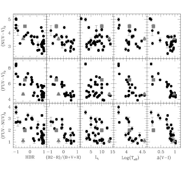
Figure 3: UV integrated colors vs five different horizontal branch classification parameters. Starting from the left: HBR as proposed by Lee, Demarque & Zinn (1994), $(B2-R)/(B+V+R)$ by Buonanno et al. (1993; 1997), horizontal branch length (L_t) by Fusi Pecci et al. (1993), temperature extension Log($T_{max}$) as introduced by Recío Blanco et al. (2006), and median horizontal branch color $\Delta(V-I)$, by Dotter et al. (2010). The grey triangle and square are NGC 2808 and NGC 1851 respectively; these have bimodal horizontal branches

A number of HB morphology classifications have been proposed over the decades. We analyze here the behavior of UV colors as a function of the most important HB parameters. Perhaps the most commonly used is $HBR=(B-R)/(B+V+R)$ introduced by Lee, Demarque, and Zinn (1994), where $V$ is the number of variables, and $B$ and $R$ are the numbers of HB stars blue-ward and red-ward of the instability strip. In the leftmost panels of Figure 3 the UV colors are shown as a function of $HBR$. The large number of clusters with $HBR\sim 1$ simply reflects our target selection as most clusters with red HBs are located at low Galactic latitude. The wide range of colors at any given value of $HBR$ arises because there is a large variety of HB morphologies even among the subset of clusters with predominantly blue HBs. The $HBR$ parameter is insensitive to the details of the color distribution of stars bluer than the RR Lyrae. The same applies to other HB morphology parameters defined on the basis of optical CMDs. Some clusters with bimodal HBs, like NGC 2808 (plotted as a gray triangle) and NGC 1851 (plotted as a gray square), have an $HBR$ value that ranks them among clusters with reddish HBs, yet they are “hot” in the UV.

We have also compared our UV colors with the HB parameter $(B2-R)/(B+V+R)$ defined by Buonanno et al. (1993; 1997), where B2 is the number of stars bluer than $(B-V)_{0}=-0.02$ (see also Catelan 2009). Data have been taken from Buonanno et al. (1997) and Preston et al. (1991). This parameter is expected to correlate more clearly with UV colors, since it is able to remove the degeneracy which characterizes HBR for clusters with extended blue HBs. In fact we find that both in $(FUV-NUV)_{0}$ and $(FUV-V)_{0}$ there is a clear trend for clusters with $(B2-R)/(B+V+R)>-0.25$, in agreement with findings by Catelan 2009 and theoretical expectations (Landsman et al. 2001). Clusters with $(B2-R)/(B+V+R)<-0.25$ are those in the ”Bimodal HB” zone (Catelan 2009). In this region in fact, we find NGC 1851 and NGC 2808, as well as other clusters with a clear bimodal HB like NGC 6864 (M75) and NGC 7006, or with a more populous red HB and a sparsely populated blue HB as NGC 1261 and NGC 362. In the latter case the extension to the blue of the HB may be actually due to contamination by background stars belonging to the Small Magellanic Clouds. A Spearman correlation rank test gives probabilities larger than $99.95\%$ for correlations with both $(FUV-NUV)_{0}$ and $(FUV-V)_{0}$. In the $(NUV-V)_{0}$ the correlation is less clear, in particular if bimodal clusters are not considered. In this case the Spearman test gives a probability P$\sim 85\%$. The $(B2-R)/(B+V+R)$ parameter is more efficient than $HBR$ in characterizing extended blue HBs. Thus, in general, it would be preferable. However we stress that $(B2-R)/(B+V+R)$ may suffer of the same limitations as $HBR$ since it is defined and measured in optical CMDs where star counts along the extreme HB blue tails could be significantly incomplete. We therefore encourage the definition of similar quantities based on a proper combination of UV and optical bands.

Fusi Pecci et al. (1993) defined several parameters describing HB blue tails (BTs) using photometry in the optical bands. In principle, their parameter L_t describing the length of BTs should correlate well with the UV light output of GCs. However, as shown in the third column of panels in Figure 3, there is no obvious correlation. The data used by Fusi Pecci et al. (1993) were not uniform and in a few cases they were based on CMDs dating back to the 1960’s. In many cases the CMDs were not deep enough to show BTs that we now know to exist. This has also been noticed by Gratton et al. (2010).

Recío-Blanco et al. (2006) included BTs in their analysis of HB morphology. They used a homogeneous deep HST survey made in the $F439W$ and $F555W$ (roughly $B$ and $V$) filters. They measured the length of BTs in terms of the maximum effective temperature ${\rm Log}(T_{\rm eff_{HB}})$ reached by the HB: the values of ${\rm Log}(T_{\rm eff_{HB}})$  were obtained by comparing in the CMDs the observed BTs with theoretical HB models. However, the optical plane is not ideal for determination of the temperatures of the hottest stars. For this reason, this parameter should be considered as a lower limit of the real HB extension, especially for the most extended BTs where the HB may be truncated in optical CMDs. Indeed, incompleteness may strongly affect clusters with a population of very hot HB stars like the Blue Hook stars. These objects have been suggested to be stars which experienced the helium-flash at high effective temperatures (see for example Moehler et al. 2004; Busso et al. 2007; Rood et al. 2008; Cassisi et al. 2009; Brown et al. 2010; Dalessandro et al. 2011; Brown et al.2012) or stars with an extremely large helium mass fraction ($Y>0.5$; D’Antona et al. 2010). However even in those cases in which incompleteness does not represent a limit, optical photometry still remains a poor measure of ${\rm Log}(T_{\rm eff_{HB}})$ for extremely hot stars. In fact, as shown for example in Dalessandro et al. (2011) in the case of NGC 2808, the value of $T_{eff}$ by Recío-Blanco et al. (2006) is underestimated by $\sim 10,000$ K. However even with this limitation, ${\rm Log}(T_{\rm eff_{HB}})$ is a useful parameter describing the UV bright population of GCs (see, e.g., Gratton et al., 2010). The fourth column of panels in Figure 3 show the UV colors as a function of ${\rm Log}(T_{\rm eff_{HB}})$ . There is an obvious correlation in the case of colors involving $FUV$ magnitudes, not so much in the case of $(NUV-V)_{0}$. This is expected, since NUV magnitudes are less sensitive than FUV to the ${\rm Log}(T_{\rm eff_{HB}})$ of the hottest stars. A Spearman test gives probabilities larger than $99.99\%$ for correlations with both $(FUV-NUV)_{0}$ and $(FUV-V)_{0}$, and $\sim 92\%$ for the correlation with $(NUV-V)_{0}$. All the clusters with ${\rm Log}(T_{\rm eff_{HB}})\ \gtrsim 4.2$ (roughly 1/3 of the sample) have approximately the same $(FUV-NUV)_{0}$ color. There is another group of clusters with $4.0\lesssim{\rm Log}(T_{\rm eff_{HB}})\ \lesssim 4.2$ with a wide range of $(FUV-NUV)_{0}$. Therefore, although the correlation between this parameter and integrated color is statistically robust for colors involving $FUV$ magnitudes, the detailed dependence of integrated color on HB morphology as defined by this parameters seems not to be monotonic.

Dotter et al. (2010) introduced the parameter $\Delta(V-I)$ to describe HB morphology. It is defined as the difference in the median colors of the HB and the red giant branch (RGB) at the level of the HB, and it is derived from a homogeneous, deep HST ACS survey in F606W and F814W (roughly $V,~{}I$). However, since BTs are almost vertical in the $(V,V-I)$ CMDs, we might expect that $\Delta(V-I)$ has problems similar to $HBR$ in characterizing the GC UV light. The rightmost column in Figure 3 shows the UV colors as a function of $\Delta(V-I)$. The correlations are good, in a statistical sense: probabilities larger than $99.99\%$ are found for $(FUV-NUV)_{0}$ and $(FUV-V)_{0}$ colors, while $\sim 93\%$ probability is obtained for a correlation with $(NUV-V)_{0}$. However the bulk of the sample is bunched up to the lower right corner of the plots. This is because, unsurprisingly, a parameter based on red optical colors distinguishes clusters with relatively red HBs from their blue counterparts, but provides very poor discrimination between clusters with blue and extremely blue HB morphologies.

4.2 Dependence on metallicity

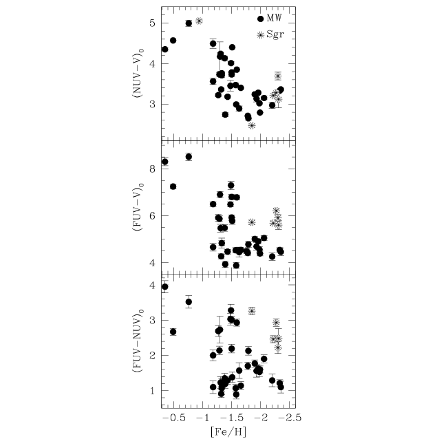
Figure 4: UV integrated colors as a function of metallicity in Carretta et al. (2009b) scale. Clusters possibly connected with the Sagittarius stream are plotted as asterisks.

In order to investigate any possible link between the UV colors and chemical compositions of the Milky Way GCs, we adopted the [Fe/H] values quoted by Carretta et al. (2009b). For Terzan 8, which is not in their sample, we used the equation listed by Carretta et al. (2009b) to convert [Fe/H] values from Zinn & West (1984) to their metallicity scale. The UV colors derived from SBP fitting are plotted as a function of metallicity in Figure 4.

First focusing on the top panel of Figure 4, one can see that, for the GCs included in this sample, $(NUV-V)_{0}$ decreases by about 2 magnitudes as [Fe/H] decreases from $\sim$ -0.7 to $\sim$ –1.5. For smaller values of [Fe/H], $(NUV-V)_{0}$ is roughly constant, or perhaps increases slightly as [Fe/H] decreases. This clear, although non-monotonic, trend of $(NUV-V)_{0}$ with metallicity is confirmed by a Spearman correlation rank test, according to which the probability of a correlation is 99.99% ($>4\sigma$). Even after removing the most metal-rich clusters (${\rm{\rm[Fe/H]}}>-1$) the probability of correlation remains significant at more than $4\sigma$. By removing from the sample the most metal-poor clusters (${\rm[Fe/H]}<-1.5$) the probability for a correlation actually increases. The more restrictive non-parametric Kendall rank correlation test also shows that there is a strong and positive correlation between $(NUV-V)_{0}$ and [Fe/H]  with a significance of $\sim 4.1\sigma$. The integrated $NUV$ radiation from GGCs is dominated by blue HB stars but it has some contribution also from turnoff and blue stragglers stars (see for example Figure 1 in Ferraro et al. 2003). The overall trend of $(NUV-V)_{0}$ as a function of metallicity seen on the top panel of Figure 4 is therefore in line with expectations from standard stellar evolution theory, as HB and turnoff stars in more metal-rich clusters are expected to be cooler and redder. This expectation was also confirmed by observations collected with ANS, OAO, and UIT, as presented by DOR95. Metallicity, however, is only one of the parameters determining the color distribution of HB stars. At least one second parameter is known to affect the color of the HB in GCs, and it can be recognized in the large spread in color for $-1.5\mathrel{\hbox{\raise 2.15277pt\hbox{$<$}\hbox to0.0pt{\hss\lower 2.15277pt\hbox{$\sim$}}}}$ [Fe/H] $\mathrel{\hbox{\raise 2.15277pt\hbox{$<$}\hbox to0.0pt{\hss\lower 2.15277pt\hbox{$\sim$}}}}-1.0$, where clusters with similar [Fe/H] can have $(NUV-V)_{0}$ differing by as much as $\sim$ 1.5 mag. The nature of this second parameter has been the subject of debate for several decades now, with candidates such as He abundance, age, mass loss, binarity, rotation, among others, being suggested in the past to explain the effect (for a review, see Catelan 2009). Recently Dotter et al. (2010) and Gratton et al. (2010) have particularly emphasized the role of age and they also stressed on the necessity of even a third parameter (the central luminosity density for the first and the He abundance for the second).

Interpretation of the dependence of colors involving $FUV$ magnitudes as a function of [Fe/H] requires a little more care. At first glance, the middle and bottom panels of Figure 4 show a less clear correlation between color and [Fe/H]. The bottom panel in particular looks like a scatter plot. It is true, though, that, $(FUV-V)_{0}$ varies by almost 5 magnitudes. Indeed, a Spearman test gives a probability $P\sim 99\%$ (corresponding to $\sim 2.3-2.5\sigma$) that $(FUV-V)_{0}$ is correlated with metallicity. The Kendall test gives correlation probability of $\sim 2.1\sigma$. The probability drops to $\sim 80\%$ if the most metal-rich clusters are excluded from the analysis. At face value, therefore, $(FUV-V)_{0}$ correlates with [Fe/H] in a similar way as $(NUV-V)_{0}$, although in a less strong or noisier fashion.

In summary, then, one finds that the behavior of GGCs in the $(FUV-V)_{0}$–[Fe/H] and $(NUV-V)_{0}$–[Fe/H] planes is essentially the same. On both planes, three sub-families of clusters can be recognized: 1) GGCs with ${\rm[Fe/H]}\mathrel{\hbox{\raise 2.15277pt\hbox{$>$}\hbox to0.0pt{\hss\lower 2.15277pt\hbox{$\sim$}}}}-1.0$, which are predominantly red ; 2) GGCs with $-1.5\mathrel{\hbox{\raise 2.15277pt\hbox{$<$}\hbox to0.0pt{\hss\lower 2.15277pt\hbox{$\sim$}}}}$ ${\rm[Fe/H]}\mathrel{\hbox{\raise 2.15277pt\hbox{$<$}\hbox to0.0pt{\hss\lower 2.15277pt\hbox{$\sim$}}}}-1.0$, the “second parameter region” (see also Fusi Pecci et al. 1993), where GGCs have a wide range of colors, about $\sim 2$ mag in $(NUV-V)_{0}$ and $\sim 4$ mag in $(FUV-V)_{0}$; and 3) GGCs with ${\rm[Fe/H]}\mathrel{\hbox{\raise 2.15277pt\hbox{$<$}\hbox to0.0pt{\hss\lower 2.15277pt\hbox{$\sim$}}}}-1.5$, which are all blue. It is worth noticing that, intermediate-metallicity ([Fe/H]$\approx-1.5$) clusters are the bluest in the three colors combinations. This was also highlighted by DOR95. The extension of their HBs (see Paper I) is compatible with their integrated colors. On average, the metal-poor (${\rm[Fe/H]}\mathrel{\hbox{\raise 2.15277pt\hbox{$<$}\hbox to0.0pt{\hss\lower 2.15277pt\hbox{$\sim$}}}}-1.7$) GCs have redder HBs than the intermediate ones. This appears to contradict expectations based on the notion that metallicity is the first parameter. Some authors interpreted this discrepancy invoking age differences among clusters. However Dotter (2008) was able to account for this behavior without invoking age differences, by using synthetic HB models and simple assumptions about the mass-loss/metallicity relation.

4.3 GCs in the Sagittarius stream

Careful inspection of the $(FUV-NUV)_{0}$ or $(FUV-V)_{0}$ vs [Fe/H] plots in Figure 4 clearly reveals that the color spread at ${\rm[Fe/H]}<-1.5$ is due to a subset of clusters (plotted as asterisks), which are systematically redder by $\sim$ 1.5 and 1.0 mag in $(FUV-NUV)_{0}$ and $(FUV-V)_{0}$, respectively, than the other GCs in the same metallicity regime. This is also confirmed if colors obtained with AP are used instead of those derived from SBP fitting. Likewise, adopting the Zinn & West (1984) metallicity scale or metallicity values by Carretta & Gratton (1997) does not affect the general behavior, even though minor differences in a cluster-to-cluster comparison can obviously come out. Interestingly these clusters (NGC 4590, NGC 5053, NGC 5466, Arp 2 and Terzan 8) are potentially connected with the Sagittarius dwarf galaxy stream (Dinescu et al. 1999, Palma et al. 2002, Bellazzini et al. 2003, Law & Majewski 2010), and thus may have an extra-Galactic origin. We stress that all these clusters have been suggested to be connected to the Sagittarius stream by at least two different authors. The other candidate Sagittarius GC is the relatively metal-rich ([Fe/H]=$-0.94$) Palomar 12, for which we were not able to get $FUV$ magnitude (see Section 3.1). Among the clusters considered here, the classification of NGC 4590 is the most uncertain. According to its metallicity, HB morphology and proper motions (Smith et al. 1998; Dinescu et al. 1999; Palma et al. 2002) it is likely associated with the Sgr stream, although Forbes & Bridges (2010) suggest that it is connected to the Canis Major dwarf. In any case, the extragalactic origin seems to be well established.

To explore the significance and meaning of this behavior we used the photometric catalogs presented in Paper I to understand how the differences in the integrated colors relate to differences in the cluster CMDs. We picked two clusters associated with the Sagittarius stream, and compared them with GGCs of similar metallicity (Figure 5). The photometric catalogs have been corrected by distance modulus and reddening values reported by H10, as done in Paper I. The HBs of the stream clusters are homogeneously populated in color and magnitude. In contrast, the GGCs show an obvious increase of star density towards higher temperatures and bluer colors. In these clusters the median color of HB stars is bluer by $(FUV-NUV)_{0}\sim 1$. This difference is qualitatively consistent with the measured discrepancy between the integrated colors. The HB star distributions differences in the GALEX CMDs are in agreement with results from optical high-resolution surveys (see Dotter et al. 2010 for example). The Sagittarius GCs do not show any systematic trend in the $(NUV-V)_{0}$ vs [Fe/H] diagram. More details about the morphology of their HBs will be presented in Paper III (R. T. Rood. et al., 2012 in preparation).

We checked also for possible differences in relative ages. For this, we used two independent papers (Salaris & Weiss 2002, and Dotter et al. 2010) containing age estimates for a large sample of GCs including most of our targets. Even though some systematic differences are present between the two age scales, within the uncertainties the clusters connected with the Sagittarius stream are classified in both cases as old and coeval with genuine GGCs in the same metallicity regime, with the only exception of Pal 12 which is $\sim 3-5$ Gyr younger. In particular, the four Sagittarius old clusters in common with Salaris & Weiss (2002; Terzan 8 has not been analyzed by the authors) have an average age of $(11.4\pm 0.6)$ Gyr which is fully compatible with the estimates for GGCs. In Dotter et al. (2010) the differences between the Galactic and the Sagittarius GCs are of the order of $\sim 0.5$ Gyr.

In addition, recent high resolution spectroscopic analysis (Carretta et al. 2010) showed that, on average, the Sagittarius clusters in our sample share the same $\alpha$-elements abundances with their Galactic twins. We used the R’-parameter reported by Gratton et al. (2010) to highlight possible differences. The R’-parameter is defined as the ratio between the number of HB stars and that of RGBs brighter than the level corresponding to $V_{\rm HB}+1$. This quantity is an indirect estimate of $Y$ (see Cassisi et al. 2003; Salaris et al. 2004), since the HB luminosity, as well as the RGB and HB lifetimes, depends on the He content. However for this comparison we preferred to use only the R’-parameter in order to avoid uncertainties that may come from the calibrations used to derive helium abundances ($(Y(R^{\prime})$) from it.

Three (NGC 4590, NGC 5053 and NGC 5466) out of the five Sagittarius clusters have been studied by Gratton et al. (2010). It is interesting to note that these clusters have R’ values smaller than other clusters with similar metallicity [Fe/H]$<-1.5$. Given the statistical uncertainties of these measurements, the difference in R’ between any two given clusters is somewhat uncertain. Therefore we performed a t-test to check the significance of the difference between the mean values of the two distributions. We find that for the clusters potentially connected with the Sgr stream $<R^{\prime}>=0.48\pm 0.01$ while for GGCs $<R^{\prime}>=0.74\pm 0.18$. The t-test gives a probability P$>99.9\%$ that they are different. We stress that it is not possible to make a final statement about this point. In fact this simple analysis suffers of low number statistics and incompleteness of our sample. Moreover the significance of the result may depend on the clusters considered to be connected with Sagittarius. However it emerges that clusters connected with Sagittarius share, on average, the same properties as the genuine GGCs, except for the R’-parameter. This difference might be an indication that those clusters have lower He abundances than GGCs in the same metallicity regime, and this is likely the main responsible of the differences in FUV integrated colors. Further analysis and estimates of the R’-parameter for the other clusters possibly associated with Sagittarius are highly desirable and could provide stronger constraints on this problem.

4.4 Dependence on other GC properties

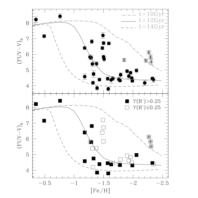
Figure 6: Top Panel. $(FUV-V)_{0}$ color as a function of metallicity as in Figure 4, with superimposed theoretical models by Lee et al. (2002). Bottom Panel. The cluster sample has been split according to the helium content: black squares are “Helium-rich” clusters ($Y(R^{\prime})>0.25$), while the open squares are the “He-poor” ones. Only clusters in common with Gratton et al. (2010) are plotted. As before, asterisks are clusters potentially associated with the Sagittarius stream.

A number of authors (Lee et al. 2002, Sohn et al. 2006, Rey et al. 2007) made use of UV integrated colors to investigate age trends in the GC systems of the Milky Way (by using OAO 2, ANS and UIT data), as well as of M31 and M87. Lee et al. (2002) and Yi et al. (2003) argued that with a proper modeling of the HB contribution to UV bands, the $(FUV-V)$ could be a good age tracer of relatively old stellar populations. The basic assumption is that the HB morphology is driven by metallicity and age. Of course a number of uncertainties may arise because of the treatment of mass loss along the upper RGB, or the presence of hot HB stars, like EHB, which are not included in these models. However under this assumption, both Lee et al. (2002) and Rey et al. (2007) were able to reproduce the UV color vs metallicity distribution of Milky Way and M31 GCs. In contrast, Sohn et al. (2006) were unable to find an acceptable match between their data for the M87 GCs and the models of Lee et al. (2002), which required unphysically old ages ($t\sim 16\,{\rm Gyr}$) to reproduce the observed color distributions. Taking advantage of our large and homogeneous sample and the high photometric accuracy of our data, in Figure 6 we compare the $(FUV-V)_{0}$-[Fe/H] distribution observed in our GC sample, with the theoretical models of Lee et al. (2002) for integrated colors of SSPs with different ages. The color-metallicity distribution of GGCs is consistent with ages $10<t<14$ Gyr, in broad agreement with the results obtained from fitting theoretical isochrones to the turnoff or the white dwarf cooling sequences (e.g., Salaris & Weiss 2002; Dotter et al. 2010). It is worth noticing that the three clusters that appear as the ”youngest” ($t\sim 10$ Gyr), according to the Lee et al. 2002 models, are those connected with the Sagittarius stream (NGC 4590, NGC 5053 and NGC 5466). As discussed above, however, they most likely are old and coeval with those in the same metallicity range, thus indicating that caution must be used to derive ages from this color-metallicity plane (Fusi Pecci et al. 1993), since other parameters play a role in distributing clusters in this diagram. The helium content certainly is one of these parameters (see for example Sohn et al. 2006, Kaviraj et al. 2007, Chung et al. 2011).

Indeed, there is now evidence that at least a few massive GCs could host multiple populations with different He abundance (see Piotto 2009 for a review). As recently shown by Chung et al. (2011; see also Kaviraj et al. 2007), helium might have a strong impact on the UV emission from an old stellar population. They suggest, in fact, that He-rich sub-populations in GCs could be able to reproduce the “UV-upturn” observed in elliptical galaxies. To check the impact of multiple populations on the observed colors we used the helium fractions $Y(R^{\prime})$ derived by the R’-parameter by Gratton et al. (2010) for the 36 clusters in common. We split our sample using $Y(R^{\prime})=0.25$ as threshold, to obtain two roughly equally populated sub-samples, with mean $Y(R^{\prime})$ of about 0.27 and 0.23. From Figure 6, it is evident that such differences in He content can have effects on UV colors equivalent to age differences of $\sim 2Gyr$.

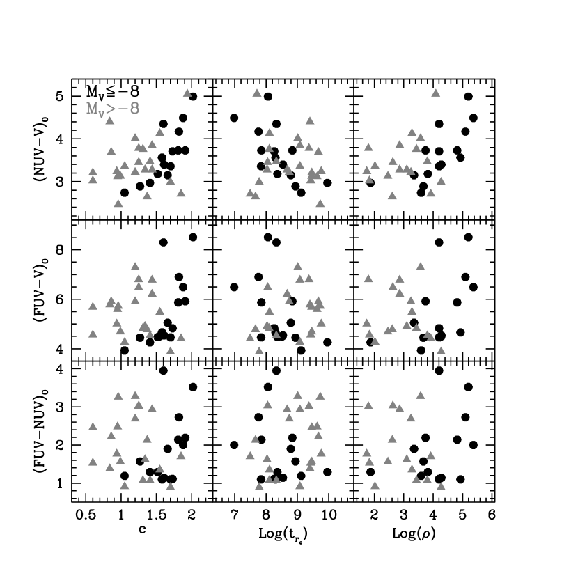
Figure 7: GALEX UV colors plotted as a function of cluster concentration, central relaxation time at $r_{c}$ and central density. The sample has been split in two sub-samples: more massive clusters ($M_{V}\leq-8$) are shown with black circles, less massive clusters are plotted as grey triangles. The four post-core collapse clusters in our sample are not plotted since the values of their concentration ($c=2.5$) is just arbitrary.

While a detailed discussion about the long standing ”HB second parameter” problem is postponed to Paper III, here we briefly consider how UV integrated colors vary with clusters parameters previously suggested to be connected with the presence of long HB BTs. Fusi Pecci et al. (1993) suggested that BTs are related to central density and concentration, and that stellar interactions somehow enhanced mass loss. Dotter et al. (2010) also suggested that the third parameter acting in modeling the HB morphologies is somehow related to the chance of interactions between stars. Figure 7 shows the GALEX colors plotted as a function of concentration $c=\log(r_{t}/r_{c})$, where $r_{c}$ is the King model core radius and $r_{t}$ is the tidal radius. While the sample as a whole shows no significant correlation, the massive cluster ($M_{V}>-8$) colors are well correlated with $c$, moving to the redder (or cooler) colors as the concentration increases. The Spearman test gives $97.5\%$ probability of correlation between $c$ and $(FUV-NUV)_{0}$, larger than $99.95\%$ with $(FUV-V)_{0}$ and about $99.8\%$ with $(NUV-V)_{0}$. This is the opposite of what we had expected from Fusi Pecci et al. (1993) and Dotter et al. (2010) interpretations. Similar results are obtained, although with lower significance, for the relaxation time and central density (Figure 7). However a direct comparison with results by Dotter et al. (2010) could not be performed, since in their analysis the authors removed the effects of metallicity and age from their parameter $\Delta(V-I)$ . We defer to Paper III for a detailed and comparative analysis.

5 Comparison with GCs in M31 and M87

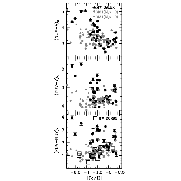
Figure 8: GALEX colors of our GGC sample (black) compared to the GCs in M31 (from Kang et al. 2011). The most massive M31 clusters (with $M_{V}\leq-9$) are plotted as grey triangles, while the less massive ones as grey circles. In the lower panel our GGC sample has been supplemented with clusters observed with ANS and OAO2 by DOR95 (open squares).

Rey et al. (2007) have used GALEX to observe GCs in M31. The authors (Kang et al. 2011) have recently published an updated catalog with a larger sample of clusters and reviewed reddening values. In Figure 8 we compare our results with data for M31 clusters classified as ”old” ($t>2Gyr$) by Caldwell et al. (2011) and we restrict the sample to clusters with $E(B-V)<0.16$, in order to avoid clusters with high reddening uncertainties.
M31 seems to show a lack of red clusters with respect to the Galaxy. However, this is likely due to the limited sensitivity of GALEX to detect relatively red populations in distant systems (see discussion in Rey et. al. 2007). Hence for the comparison we focus on the bluest systems, $(FUV-NUV)_{0}\lower 2.15277pt\hbox{$\;\buildrel<\over{\sim}\;$}1.5$, $(FUV-V)_{0}\lower 2.15277pt\hbox{$\;\buildrel<\over{\sim}\;$}5$ and $(NUV-V)_{0}\lower 2.15277pt\hbox{$\;\buildrel<\over{\sim}\;$}3.5$, which, for the GGCs, correspond to a metallicity range $-2.5<{\rm[Fe/H]}<-1.0$. In this metallicity regime the distributions in the Milky Way and in M31 are quite similar. The bluest colors reached are essentially the same, and the distributions show little variations with metallicity. Three M31 clusters lie almost in the same region as GCs connected with the Sagittarius dwarf in the $(FUV-V)_{0}$-[Fe/H] plane. They are G 327, B 366 and interestingly B 009 that is known to be projected against the dwarf spheroidal galaxy NGC 205. Unfortunately CMDs are available only for B 366 (Perina et al. 2009). This is an old cluster with a red HB and possibly a very mild blue extension, which makes it compatible with its redder UV colors.

The case is very different at higher metallicity, ${\rm[Fe/H]}>-1$. In the Milky Way sample there are only red GGCs, while in M31 there are many blue GCs.
In order to make the comparison with M31 GCs as complete as possible, we have supplemented our GALEX sample with 12 additional GGCs from DOR95, not observed by GALEX because of the target selection limitations discussed in Section 2. First, we converted the ANS and OAO 2 magnitudes from the STMAG to the ABMAG system and we checked that no systematic color offsets or trends are present for the (15) GCs in common. The average difference results to be $\Delta(FUV-NUV)_{0}=0.08$ and is fully consistent with the reported errors. Then, we adopted the ANS and OAO 2 magnitudes given in Table 1 of DOR95 and we corrected these values by using the color excess $E(B-V)$ quoted by H10. So as not to introduce additional errors through the $V$ magnitudes, we consider only the $(FUV-NUV)$ color. The results are shown as open squares in the lower panel of Figure 8 and demonstrate that (at least) two GCs, namely NGC 6388 and NGC 6441, in the Galaxy have colors comparable to those of M31 at ${\rm[Fe/H]}>-1$. Still, M31 appears to have many more hot metal-rich GCs. Why would that be the case? As shown in Figure 8 roughly half of the blue, metal-rich M31 GCs are indeed quite massive ($M_{V}\leq-9$). Hence, the relative paucity of hot, metal-rich GCs in the Milky Way could be due in part (but only in part) to the fact that there are only two massive metal-rich clusters in our supplemented sample. It is also possible that many GGCs with high metallicity and a blue HB are missed because of their location towards highly extinguished regions of the Galaxy.

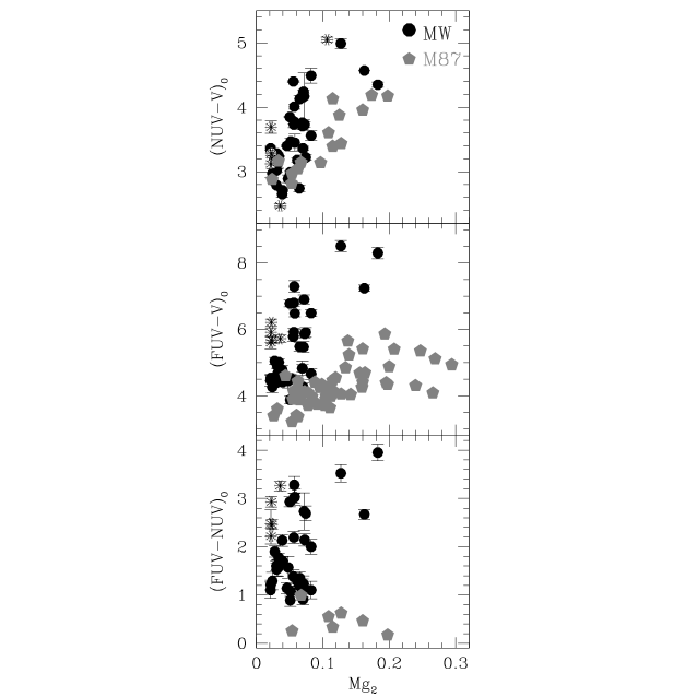
Figure 9: UV colors of GGCs (black dots and asterisks) compared to those of M87 (grey pentagons) observed by Sohn et al. (2006), as a function of the $Mg_{2}$ metallicity index.

We also compare GGC colors measured with GALEX with those obtained for the giant elliptical galaxy M87 using HST STIS images (Sohn et al. 2006). We converted those magnitudes from the STMAG to the ABMAG photometric system. In order to perform a direct comparison, we transformed [Fe/H] values to the metallicity indicator $Mg_{2}$ using equation A1 in the Appendix of Sohn et al. (2006). As shown in Figure 9, M87 GCs are on average bluer by $\sim 1.5$ mag both in $(FUV-NUV)_{0}$ and $(FUV-V)_{0}$, while they do not show any appreciable difference in $(NUV-V)_{0}$. These differences are consistent with what observed by Sohn et al. (2006) in comparison with the DOR95 sample. On the basis of what we discussed in Section 4.3, we may suppose that M87 GCs are on average older or have a higher He content than the Milky Way objects. As noted above, the age-metallicity grid of theoretical predictions provides realistic ages for the M87 GCs only when the effect of Helium is taken into account (see Figure 2 in Chung et al. 2011; Kaviraj et al. 2007).

From the comparison between GGCs and those belonging to three other galaxies (the Sagittarius dwarf, M31 and M87), different behaviors emerged. In fact the clusters associated with the Sagittarius dwarf are on average redder than the MW ones, the M31 clusters have colors which are comparable to those of the GGCs, while the M87 star systems are bluer. We note that there may be a possible trend between the mass of the host galaxy and the color distribution of its globulars, in the sense that the higher is the galaxy mass, the bluer are the GC UV colors. In fact M87 (with the bluer systems) is a super-giant elliptical that is about two orders of magnitude more massive than the Milky Way ($1.7\times 10^{13}<M/M_{\odot}<4.0\times 10^{13}$; Fabricant et al., 1980), while Sagittarius ($\sim 1.6\times 10^{8}M_{\odot}$; Law & Majewski, 2010) with the reddest sample of GCs (although quite small), is a dwarf galaxy, and M31 ($3.7\times 10^{11}<M/M_{\odot}<2.5\times 10^{12}$; Côté et al., 2000) and the Galaxy ($2.4\times 10^{11}<M/M_{\odot}<1.2\times 10^{12}$; Little & Tremaine, 1987; Kochanek, 1996) representing intermediate cases. We argued that most of the observed differences between colors involving the $FUV$ band are explainable invoking different Helium contents. This would lead us to speculatively think that galaxies with larger masses may have, on average, more He-rich populations. In that case, He abundance differences could be a by-product of chemical evolution differences, in some way connected to the mass of the host galaxy. This could be also connected with the formation and dynamical history of clusters in galaxies with different masses, as suggested by Valcarce & Catelan (2011). In particular they argue that clusters hosted by more massive galaxies are more likely to undergo a more complex history of star formation thus having a larger spread in stellar populations properties.

6 Summary

As part of a project aimed at studying the properties of hot stellar populations in the Milky Way GCs (see Paper I), we have presented UV integrated colors obtained with GALEX for 44 clusters spanning a wide range of metallicities ($-2.5<{\rm[Fe/H]}<-0.4$), HB morphologies, structural and dynamical parameters. This represents the largest homogeneous catalog of UV photometry ever built for GGCs.

We compared the behavior of UV colors with several parameters characterizing the morphology of the HB. As expected, there are general correlations, in particular between $(FUV-V)_{0}$ and the $(B2-R)/(B+V+R)$ parameter defined by Buonanno et al. (1993; 1997) and the HB temperature extension $T_{\rm eff}$ defined by Recío Blanco et al. (2005). There is also a significant correlation with the $\Delta(V-I)$ parameter (Dotter et al. 2010), but, as expected, this parameter is insensitive to HBs with extreme blue extensions.

In all color combinations, the bluest clusters are those in the intermediate metallicity regime ($-1.5<{\rm[Fe/H]}<-1$). This is in agreement with DOR95 and with the L_t parameters measured by Fusi Pecci et al. (1993). In the $(NUV-V)_{0}$-${\rm[Fe/H]}$ plane, clusters more metal rich than ${\rm[Fe/H]}\sim-1.5$ show a clear and significant linear correlation with cluster becoming redder as metallicity increases, while there is an opposite trend in the metal-poor regime. The combinations of colors involving the $FUV$ appear more scattered, but a reasonable and similar correlation with metallicity at ($2.5\sigma$ level) has been also found in these cases. All the clusters suspected to be connected with the Sagittarius dwarf spheroidal (NGC 4590, NGC 5053, NGC 5466, Arp 2 and Terzan 8) are typically $\sim 1.5$ mag redder in $FUV$ colors than systems with similar iron content. No appreciable differences are found in $(NUV-V)_{0}$. Studies from different groups suggest that Sagittarius clusters and their galactic counterparts are coeval, while GGCs are on average more He-rich than the Sagittarius sub-set. This would tentatively be interpreted as due to a different environment in which they formed.

With the aim of showing how sensitive ages derived from UV colors may be to assumptions about helium abundance, we compared our colors with evolutionary models of SSP by Lee et al. (2002). The color-metallicity distribution of GGCs can be reproduced by assuming an average age of $\sim 12$ Gyr, with a spread of about $\pm 2\,{\rm Gyr}$. Alternatively, in the framework in which some GCs have experienced self-enrichment from material ejected from AGBs or fast-rotating massive stars (Ventura & D’Antona 2008; Decressin et al. 2007), the color spread is consistent with different He content. In particular, we show that an overabundance of helium ($\Delta Y(R^{\prime})\sim 0.05$ ) can mimic an age difference $\Delta t\sim 2\,{\rm Gyr}$.

The UV colors of GGCs are consistent with those obtained by GALEX for M31 clusters (Rey et al. 2007; Kang et al. 2011), at least in the intermediate/low metallicity regime. At ${\rm[Fe/H]}>-1$, M31 GCs are systematically bluer by 1–2 mag, behaving like massive MW clusters with bimodal HBs, such as NGC 6388 and NGC 6441. As already noticed by Sohn et al. (2006), M87 GCs are on average bluer than GGCs. This might be the signature of different chemical abundances impressed on the ”integrated” properties of GCs. In particular we speculate that He abundance may be correlated with the mass of the host galaxy, being higher in GCs belonging to higher mass galaxies.

The authors dedicate this paper to the memory of co-author Bob Rood, a pioneer in the theory of the evolution of low mass stars, and a friend, who sadly passed away on 2 November 2011.
We thank the anonymous referee for the useful comments and suggestions. The authors warmly thank M. Bellazzini and F. Fusi Pecci for useful discussions that improved the presentation of the results. We are grateful to M. Catelan for providing us informations about HB parameters. This work is based on observations made with the NASA Galaxy Evolution Explorer. GALEX is operated for NASA by the California Institute of Technology under NASA contract NAS5- 98034. This research is part of the project COSMIC-LAB funded by the European Research Council (under contract ERC-2010-AdG-267675). E.D. thanks the hospitality and support from Gemini Observatory where most of this work was developed, during two extended visits in 2009 and 2010, and a shorter visit in 2011. R.P.S. acknowledges funding by GALEX grants $\#$ NNG05GE50G and NNX08AW42G and support from Gemini Observatory, which is operated by the Association of Universities for Research in Astronomy, Inc., on behalf of the international Gemini partnership of Argentina, Australia, Brazil, Canada, Chile, the United Kingdom, and the United States of America. S.T.S. acknowledges support for this work from the GALEX Guest Investigator Program under NASA grant NNX07AP07G.

Figure 2: Comparison between magnitudes and colors obtained by using surface brightness profiles fitting (SBP; Sect. 3.1) and aperture photometry (AP; Sect. 3.2). COL stands for (FUV-NUV). The few clusters showing large differences are marked with large crosses.

Figure 5: Comparison between GALEX CMDs of two GCs connected with the Sagittarius stream (upper panels), and GGCs in the same metallicity regime (lower panels).

CLUSTER	[Fe/H]	$E(B-V)$	$V_{t,0}$	$(FUV-NUV)_{0}$	$(FUV-V)_{0}$	$(NUV-V)_{0}$
NGC 104	-0.76	0.04	4.09	3.52	8.51	4.99
NGC 1261	-1.27	0.01	8.63	2.69	5.91	3.22
NGC 1851	-1.18	0.02	7.23	2.00	6.49	4.49
NGC 1904	-1.58	0.01	8.16	0.89	3.88	2.99
NGC 2298	-1.96	0.14	8.89	1.62	4.91	3.28
NGC 2419	-2.20	0.08	10.05	1.29	4.26	2.97
NGC 288	-1.32	0.03	8.13	0.91	4.27	3.36
NGC 2808	-1.18	0.22	5.69	1.10	4.66	3.56
NGC 362	-1.30	0.05	6.58	2.73	6.90	4.17
NGC 4147	-1.78	0.02	10.74	1.70	4.41	2.71
NGC 4590	-2.27	0.05	7.96	2.93	6.21	3.28
NGC 5024	-2.06	0.02	7.79	1.90	5.05	3.15
NGC 5053	-2.30	0.01	9.96	2.22	5.91	3.69
NGC 5272	-1.50	0.01	6.39	2.19	5.92	3.73
NGC 5466	-2.31	0.00	9.70	2.48	5.60	3.12
NGC 5897	-1.90	0.09	8.52	1.77	5.01	3.24
NGC 5904	-1.33	0.03	5.95	1.11	4.83	3.71
NGC 5986	-1.63	0.28	6.92	1.57	4.45	2.89
NGC 6101	-1.98	0.05	10.08	1.53	4.56	3.02
NGC 6218	-1.33	0.19	6.07	1.07	4.83	3.76
NGC 6229	-1.43	0.01	9.86	1.29	4.47	3.18
NGC 6235	-1.38	0.31	7.20	1.35	5.48	4.13
NGC 6254	-1.57	0.28	4.98	1.07	4.53	3.47
NGC 6273	-1.76	0.38	5.57	—	4.49	—
NGC 6284	-1.31	0.28	7.43	1.23	5.47	4.24
NGC 6341	-2.35	0.02	6.52	1.10	4.46	3.36
NGC 6342	-0.49	0.46	10.01	2.67	7.24	4.57
NGC 6356	-0.35	0.28	7.42	3.95	8.30	4.35
NGC 6397	-1.99	0.18	5.17	1.60	4.39	2.79
NGC 6402	-1.39	0.60	5.73	1.19	3.93	2.74
NGC 6535	-1.79	0.34	9.85	2.13	4.78	2.65
NGC 6584	-1.50	0.10	8.17	3.28	7.29	4.01
NGC 6809	-1.93	0.08	6.49	1.56	4.69	3.13
NGC 6864	-1.29	0.16	8.26	2.14	5.87	3.73
NGC 6981	-1.48	0.05	8.96	3.03	6.48	3.45
NGC 7006	-1.46	0.05	10.46	2.93	6.78	3.85
NGC 7089	-1.66	0.06	6.25	1.14	4.54	3.40
NGC 7099	-2.33	0.03	7.10	1.21	4.54	3.33

CLUSTER	[Fe/H]	$E(B-V)$	$V_{t,0}$	$(FUV-NUV)_{0}$	$(FUV-V)_{0}$	$(NUV-V)_{0}$
Pal 11	-0.45	0.35	7.54	—	—	—
Pal 12	-0.81	0.02	11.89	—	—	5.05
NGC 7492	-1.69	0.00	10.48	1.38	5.78	4.40
IC 4499	-1.62	0.23	8.56	3.01	6.80	3.78
Terzan 8	-2.22	0.12	11.54	2.46	5.68	3.21
Arp 2	-1.74	0.10	12.41	3.26	5.72	2.47

Note. — Integrated reddening corrected UV colors and integrated V magnitudes obtained by fitting the surface brightness profiles (see Section 2.1 for more details). For reddening correction we used the following coefficients: $R_{FUV}=8.2$, $R_{NUV}=9.2$ and $R_{V}=3.1$ (Cardelli et al. 1989). The adopted $E(B-V)$ values are from H10, while [Fe/H] value are from Carretta et al. (2009b). For the three clusters with large discrepancies between SBP and AP magnitudes we report also AP colors. For 47 Tuc AP colors are $(FUV-NUV)_{0}=2.72$, $(FUV-V)_{0}=7.49$, $(NUV-V)_{0}=4.77$. For NGC 1851 $(FUV-NUV)_{0}=1.14$, $(FUV-V)_{0}=4.95$, $(NUV-V)_{0}=3.81$ and for NGC 6864 $(FUV-NUV)_{0}=1.60$, $(FUV-V)_{0}=4.73$, $(NUV-V)_{0}=3.13$.

References

- Alonso-García et al. (2012) Alonso-García, J., Mateo, M., Sen, B., et al. 2012, AJ, 143, 70
- Bellazzini et al. (2003) Bellazzini, M., Ferraro, F. R., & Ibata, R. 2003, AJ, 125, 188
- Bellazzini (2007) Bellazzini, M. 2007, A&A, 473, 171
- Bertola et al. (1982) Bertola, F., Capaccioli, M., & Oke, J. B. 1982, ApJ, 254, 494
- Brown et al. (2010) Brown, T. M., Sweigart, A. V., Lanz, T., et al. 2010, ApJ, 718, 1332
- Brown et al. (2012) Brown, T. M., Lanz, T., Sweigart, A. V., et al. 2012, ApJ, 748, 85
- Buonanno (1993) Buonanno, R. 1993, The Globular Cluster-Galaxy Connection, 48, 131
- Buonanno et al. (1997) Buonanno, R., Corsi, C., Bellazzini, M., Ferraro, F. R., & Pecci, F. F. 1997, AJ, 113, 706
- Busso et al. (2007) Busso, G., Cassisi, S., Piotto, G., et al. 2007, A&A, 474, 105
- Caldwell et al. (2011) Caldwell, N., Schiavon, R., Morrison, H., Rose, J. A., & Harding, P. 2011, AJ, 141, 61
- Cardelli et al. (1989) Cardelli, J. A., Clayton, G. C., & Mathis, J. S. 1989, ApJ, 345, 245
- Carretta & Gratton (1997) Carretta, E., & Gratton, R. G. 1997, A&AS, 121, 95
- Carretta et al. (2009a) Carretta, E., Bragaglia, A., Gratton, R. G., et al. 2009, A&A, 505, 117
- Carretta et al. (2009b) Carretta, E., Bragaglia, A., Gratton, R., D’Orazi, V., & Lucatello, S. 2009, A&A, 508, 695
- Carretta et al. (2010) Carretta, E., Bragaglia, A., Gratton, R.G. et al. 2010, A&A, 520, 95
- Cassisi et al. (2003) Cassisi, S., Salaris, M., & Irwin, A. W. 2003, ApJ, 588, 862
- Cassisi et al. (2009) Cassisi, S., Salaris, M., Anderson, J., et al. 2009, ApJ, 702, 1530
- Castellani & Cassatella (1987) Castellani, V., & Cassatella, A. 1987, Exploring the Universe with the IUE Satellite, 129, 637
- Catelan (2009) Catelan, M. 2009, Ap&SS, 320, 261
- Chung et al. (2011) Chung, C., Yoon, S.-J., & Lee, Y.-W. 2011, ApJ, 740, L45
- Code & Welch (1979) Code, A. D., & Welch, G. A. 1979, ApJ, 228, 95
- Contreras Ramos et al. (2012) Contreras Ramos, R., Ferraro, F. R., Dalessandro, E., Lanzoni, B., & Rood, R. T. 2012, ApJ, 748, 91
- Côté et al. (2000) Côté, P., Mateo, M., Sargent, W. L. W., & Olszewski, E. W. 2000, ApJ, 537, L91
- Dalessandro et al. (2008) Dalessandro, E., Lanzoni, B., Ferraro, F. R., et al. 2008, ApJ, 677, 1069
- Dalessandro et al. (2011) Dalessandro, E., Salaris, M., Ferraro, F. R., Cassisi, S., Lanzoni, B., Rood, R. T., Fusi Pecci, F., & Sabbi, E. 2011, MNRAS, 410, 694
- D’Antona et al. (2010) D’Antona, F., Caloi, V., & Ventura, P. 2010, MNRAS, 405, 2295
- de Boer (1982) de Boer, K. S. 1982, A&AS, 50, 247
- Decressin et al. (2007) Decressin, T., Meynet, G., Charbonnel, C., Prantzos, N., & Ekström, S. 2007, A&A, 464, 1029
- Dinescu et al. (1999) Dinescu, D. I., Girard, T. M., & van Altena, W. F. 1999, AJ, 117, 1792
- Dixon et al. (1995) Dixon, W. V. D., Davidsen, A. F., & Ferguson, H. C. 1995, ApJ, 454, L47
- Dorman et al. (1995) Dorman, B., O’Connell, R. W., & Rood, R. T. 1995, ApJ, 442, 105 (DOR95)
- Dotter (2008) Dotter, A. 2008, ApJ, 687, L21
- Dotter et al. (2010) Dotter, A., et al. 2010, ApJ, 708, 698
- Fabricant et al. (1980) Fabricant, D., Lecar, M., & Gorenstein, P. 1980, ApJ, 241, 552
- Ferraro et al. (1997) Ferraro, F. R., Paltrinieri, B., Fusi Pecci, F., et al. 1997, A&A, 324, 915
- Ferraro et al. (1998) Ferraro, F. R., Paltrinieri, B., Pecci, F. F., Rood, R. T., & Dorman, B. 1998, ApJ, 500, 311
- Ferraro et al. (1999) Ferraro, F. R., Paltrinieri, B., Rood, R. T., & Dorman, B. 1999, ApJ, 522, 983
- Ferraro et al. (2001) Ferraro, F. R., D’Amico, N., Possenti, A., Mignani, R. P., & Paltrinieri, B. 2001, ApJ, 561, 337
- Ferraro et al. (2003) Ferraro, F. R., Sills, A., Rood, R. T., Paltrinieri, B., & Buonanno, R. 2003, ApJ, 588, 464
- Ferraro et al. (2004) Ferraro, F. R., Sollima, A., Pancino, E., et al. 2004, ApJ, 603, L81
- Ferraro et al. (2009) Ferraro, F. R., Dalessandro, E., Mucciarelli, A., et al. 2009, Nature, 462, 483
- Fusi Pecci et al. (1993) Fusi Pecci, F., Ferraro, F. R., Bellazzini, M., Djorgovski, S., Piotto, G., & Buonanno, R. 1993, AJ, 105, 1145
- Goldsbury et al. (2010) Goldsbury, R., Richer, H. B., Anderson, J., Dotter, A., Sarajedini, A., & Woodley, K. 2010, AJ, 140, 1830
- Gratton et al. (2010) Gratton, R. G., Carretta, E., Bragaglia, A., Lucatello, S., & D’Orazi, V. 2010, A&A, 517, A81
- Greggio & Renzini (1990) Greggio, L., & Renzini, A. 1990, ApJ, 364, 35
- Han et al. (2007) Han, Z., Podsiadlowski, P., & Lynas-Gray, A. E. 2007, MNRAS, 380, 1098
- Harris (1996) Harris, W. E. 1996, AJ, 112, 1487 (H10)
- Hill et al. (1992) Hill, R. S., et al. 1992, ApJ, 395, L17
- Kang et al. (2011) Kang, Y., Rey, S.-C., Bianchi, L., et al. 2011, arXiv:1112.2944
- Kaviraj et al. (2007) Kaviraj, S., Sohn, S. T., O’Connell, R. W., et al. 2007, MNRAS, 377, 987
- Kochanek (1996) Kochanek, C. S. 1996, ApJ, 457, 228
- Landsman et al. (1992) Landsman, W. B., et al. 1992, ApJ, 395, L21
- Landsman et al. (2001) Landsman, W. B., Catelan, M., O’Connell, R. W., Pereira, D., & Stecher, T. P. 2001, Bulletin of the American Astronomical Society, 33, 1385
- Lanzoni et al. (2007) Lanzoni, B., Dalessandro, E., Ferraro, F. R., Miocchi, P., Valenti, E., & Rood, R. T. 2007, ApJ, 668, L139
- Law & Majewski (2010) Law, D. R., & Majewski, S. R. 2010, ApJ, 718, 1128
- Lee et al. (1994) Lee, Y.-W., Demarque, P., & Zinn, R. 1994, ApJ, 423, 248
- Lee et al. (1999) Lee, Y.-W., Joo, J.-M., Sohn, Y.-J., et al. 1999, Nature, 402, 55
- Lee et al. (2002) Lee, H.-c., Lee, Y.-W., & Gibson, B. K. 2002, AJ, 124, 2664
- Little & Tremaine (1987) Little, B., & Tremaine, S. 1987, ApJ, 320, 493
- McLaughlin & van der Marel (2005) McLaughlin, D. E., & van der Marel, R. P. 2005, ApJS, 161, 304 (MVM05)
- Moehler et al. (2004) Moehler, S., Sweigart, A. V., Landsman, W. B., Hammer, N. J., & Dreizler, S. 2004, A&A, 415, 313
- Morrissey et al. (2005) Morrissey, P., et al. 2005, ApJ, 619, L7
- Norris et al. (1996) Norris, J. E., Freeman, K. C., & Mighell, K. J. 1996, ApJ, 462, 241
- Noyola & Gebhardt (2006) Noyola, E., & Gebhardt, K. 2006, AJ, 132, 447
- O’Connell et al. (1997) O’Connell, R. W., et al. 1997, AJ, 114, 1982
- O’Connell (1999) O’Connell, R. W. 1999, ARA&A, 37, 603
- Palma et al. (2002) Palma, C., Majewski, S. R., & Johnston, K. V. 2002, ApJ, 564, 736
- Parise et al. (1994) Parise, R. A., et al. 1994, ApJ, 423, 305
- Perina et al. (2009) Perina, S., Federici, L., Bellazzini, M., et al. 2009, A&A, 507, 1375
- Piotto (2009) Piotto, G. 2009, IAU Symposium, 258, 233
- Preston et al. (1991) Preston, G. W., Shectman, S. A., & Beers, T. C. 1991, ApJ, 375, 121
- Recío-Blanco et al. (2006) Recío-Blanco, A., Aparicio, A., Piotto, G., de Angeli, F., & Djorgovski, S. G. 2006, A&A, 452, 875
- Rey et al. (2007) Rey, S.-C., et al. 2007, ApJS, 173, 643
- Rich et al. (2005) Rich, R. M., et al. 2005, ApJ, 619, L107
- Rood et al. (2008) Rood, R. T., Beccari, G., Lanzoni, B., Ferraro, F. R., Dalessandro, E., & Schiavon, R. P. 2008, Mem. Soc. Astron. Italiana, 79, 383
- Sanna et al. (2012) Sanna, N., Dalessandro, E., Lanzoni, B., et al. 2012, MNRAS, 2579
- Salaris & Weiss (2002) Salaris, M., & Weiss, A. 2002, A&A, 388, 492
- Salaris et al. (2004) Salaris, M., Riello, M., Cassisi, S., & Piotto, G. 2004, A&A, 420, 911
- Schiavon et al. (2012) Schiavon, R. P., Dalessandro, E., Sohn, S. T., et al. 2012, AJ, 143, 121 (Paper I)
- Smith et al. (1998) Smith, E. O., Rich, R. M., & Neill, J. D. 1998, AJ, 115, 2369
- Sohn et al. (2006) Sohn, S. T., O’Connell, R. W., Kundu, A., Landsman, W. B., Burstein, D., Bohlin, R. C., Frogel, J. A., & Rose, J. A. 2006, AJ, 131, 866
- Stetson (1987) Stetson, P. B. 1987, PASP, 99, 191
- Valcarce & Catelan (2011) Valcarce, A. A. R., & Catelan, M. 2011, A&A, 533, A120
- van Albada et al. (1981) van Albada, T. S., de Boer, K. S., & Dickens, R. J. 1981, MNRAS, 195, 591
- Ventura & D’Antona (2008) Ventura, P., & D’Antona, F. 2008, MNRAS, 385, 2034
- Wallerstein et al. (2003) Wallerstein, G., Gonzalez, G., & Shetrone, M. D. 2003, arXiv:astro-ph/0305143
- Welch & Code (1972) Welch, G. A., & Code, A. D. 1972, Scientific results from the orbiting astronomical observatory (OAO-2), 310, 541
- Welch & Code (1980) Welch, G. A., & Code, A. D. 1980, ApJ, 236, 798
- Whitney et al. (1994) Whitney, J. H., et al. 1994, AJ, 108, 1350
- Wilson (1975) Wilson, C. P. 1975, AJ, 80, 175
- Yi (2003) Yi, S. K. 2003, ApJ, 582, 202
- Zinn & West (1984) Zinn, R., & West, M. J. 1984, ApJS, 55, 45