Polymers, KPZ equation, fluctuation statistics, extremal events

Directed polymer near a hard wall and KPZ equation in the half-space

Abstract

We study the directed polymer with fixed endpoints near an absorbing wall, in the continuum and in presence of disorder, equivalent to the KPZ equation on the half space with droplet initial conditions. From a Bethe Ansatz solution of the equivalent attractive boson model we obtain the exact expression for the free energy distribution at all times. It converges at large time to the Tracy Widom distribution $F_{4}$ of the Gaussian Symplectic Ensemble (GSE). We compare our results with numerical simulations of the lattice directed polymer, both at zero and high temperature.

Much progress was achieved recently in finding exact solutions in one dimension for noisy growth models in the Kardar-Parisi-Zhang (KPZ) universality class [1, 2], and for the closely related equilibrium statistical mechanics problem of the directed polymer (DP) in presence of quenched disorder [3]. The KPZ class has been explored in several recent experiments [4, 5], and the DP has found applications ranging from biophysics [6] to describing the glass phase of pinned vortex lines [7] and magnetic walls [8]. The height of the growing interface, $h(x,t)$, corresponds to the free energy of a DP of length $t$ starting at point $x$, under a mapping which is exact in the continuum (Cole-Hopf), as well as for some discrete realizations. Not only the scaling exponents $h\sim t^{1/3}$, $x\sim t^{2/3}$ are known [9, 10], but also the one-point (and in some cases the many-point) probability distribution (PDF) of the height have been obtained [16, 17]. Their dependence in the initial condition was found to exhibit remarkable universality at large time, with only a few subclasses, most being related to Tracy Widom (TW) distributions [15] of largest eigenvalues of random matrices. Most of these subclasses were initially discovered in a discrete growth model (the PNG model) [11, 12, 13] which can be mapped onto the statistics of random permutations [14], and a zero temperature lattice DP model [10]. Recently, exact solutions have been obtained directly in the continuum at arbitrary time $t$, for the droplet [18, 19, 20, 21], flat [22, 23] and stationary [24] initial conditions. The PDF of the height $h(x,t)$ converges at large time to $F_{2}$, the Gaussian unitary ensemble (GUE), and to $F_{1}$, the Gaussian orthogonal ensemble (GOE) universal TW distributions, for droplet and flat initial conditions respectively. One useful method which led to these solutions introduces $n$ replica and maps the DP problem to the Lieb Liniger model, i.e. the quantum mechanics of $n$ bosons with mutual delta-function attraction, a model which can be solved using the Bethe Ansatz.

The KPZ equation on the half line $x>0$, equivalently a DP in presence of a wall, is also of great interest. In the statistical mechanics context constrained fluctuations are important for the study of fluctuation-induced (Casimir) forces [25, 26] and for extreme value statistics. In the surface growth context one can study an interface pinned at a point, or an average growth rate which jumps across a boundary. The half space problem was studied previously in a discrete version, for the (symmetrized) random permutations/PNG model [28, 27] and found to also involve TW distributions in the limit of large system size. In order to exhibit full KPZ universality, it is important to solve the problem directly in the continuum, i.e. for the KPZ equation itself. Furthermore, previous approaches did not provide any information about the finite time behavior which is also universal [29].

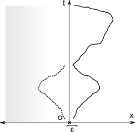
Figure 1: Solid line: a DP with both endpoints fixed at small $x=\epsilon$ with a hard wall at $x=0$: the DP probability vanishes at the wall. Dashed line: mirror image discussed at the end.

The aim of this Letter is to present a solution of the directed polymer problem in the continuum in presence of a hard wall (absorbing wall) using the Bethe ansatz (BA). Equivalently, we obtain the one-point height probability distribution for the KPZ equation on the half line $x>0$ with fixed large negative value of $h$ or of $-\nabla h$ (i.e. a small contact angle) at $x=0$. For simplicity we study a DP with both endpoints fixed - which corresponds to the droplet initial condition in KPZ - near the wall. We do not consider the case of the attractive wall although we briefly mention it at the end. We obtain an exact expression for the generating function of the moments of the DP partition sum as a Fredholm Pfaffian, from which we extract the PDF of the free energy of the DP (height of KPZ) at all times. We then show that this PDF converges to $F_{4}$, the Tracy Widom distribution of the largest eigenvalue of the Gaussian Symplectic Ensemble (GSE). The calculation is performed on the DP formulation, the consequences for the KPZ equation being detailed at the end. Our results are checked against numerics on a discrete DP model, both at high and zero temperature, thereby confirming universality. Some consequences for extreme value statistics are discussed. Note that this is the first occurrence of the $F_{4}$ distribution and of the GSE within a continuum BA calculation. It is consistent with the results of [28, 27] for the discrete model and confirms that these belong to the same universality class than the continuum KPZ equation on the half space, solved here for all times.

Directed polymer: analytical solution. We consider the partition function of a DP at temperature $T$ in the continuum, i.e the sum over positive paths $x(\tau)\in R^{+}$ starting at $x(0)=y$ and ending at $x(t)=x$

$$Z(x,y,t)=\int_{x(0)=y}^{x(t)=x}Dx(\tau)e^{-\frac{1}{T}\int_{0}^{t}d\tau[\frac{1}{2}(\frac{dx}{d\tau})^{2}+V(x(\tau),\tau)]}\,,$$ (1)

with initial condition $Z(x,y,0)=\delta(x-y)$. The hard wall is implemented by requiring that $Z(0,y,t)=Z(x,0,t)=0$. The random potential $V(x,t)$ is centered gaussian with correlator $\overline{V(x,t)V(x^{\prime},t)}=\bar{c}\delta(t-t^{\prime})\delta(x-x^{\prime})$. The natural units for the continuum model are $t^{*}=2T^{5}/\bar{c}^{2}$ and $x^{*}=T^{3}/\bar{c}$ which allow to remove $T$ and set $\bar{c}=1$ The time (i.e. polymer length) dependence is embedded in a single dimensionless parameter:

$$\lambda=(t/4t^{*})^{1/3}$$ (2)

as defined in our previous works [19, 22, 23] and in [20].

Replicating (1) and averaging over disorder one finds [30] that the $n$-th integer moment of the DP partition sum can be expressed as a quantum mechanical expectation for $n$ particles described by the attractive Lieb-Liniger Hamiltonian [31]

$$H_{n}=-\sum_{j=1}^{n}\frac{\partial^{2}}{\partial{x_{j}^{2}}}-2\bar{c}\sum_{1\leq i<j\leq n}\delta(x_{i}-x_{j}).$$ (3)

in natural units (for the moment not rescaling by $\bar{c}$, as in [19]). The moments of the partition sum with both endpoints fixed at $x$ can be written as:

$$\overline{Z(x,x,t)^{n}}=\sum_{\mu}|\Psi_{\mu}(x,..,x)|^{2}\frac{e^{-tE_{\mu}}}{||\mu||^{2}}$$ (4)

i.e. a sum over the un-normalized eigenfunctions $\Psi_{\mu}$ (of norm denoted $||\mu||$) of $H_{n}$ with energies $E_{\mu}$. Here we used the fact that only symmetric (i.e. bosonic) eigenstates contribute. In presence of a hard wall at $x=0$ we must impose that $\Psi_{\mu}(x_{1},..,x_{n})$ vanishes when any of the $x_{j}$ vanishes. This case can also be solved, by a simple generalization of the standard BA [32, 33]. The Bethe states $\Psi_{\mu}$ are superpositions of plane waves [31] over all permutations $P$ of the rapidities $\lambda_{j}$ ($j=1,..n$), with here an additional summation over $\pm\lambda_{j}$. The eigenfunctions read, for $x_{1}<..<x_{n}$:

$$\Psi_{\mu}(x_{1},..,x_{n})=\frac{1}{(2i)^{n-1}}\sum_{P\in S_{n}}\sum_{\epsilon_{2},..\epsilon_{n}=\pm 1}\epsilon_{2}..\epsilon_{n}$$ (5)

$$\times A_{\lambda_{P_{1}},\epsilon_{2}\lambda_{P_{2}},..,\epsilon_{n}\lambda_{P_{n}}}\sin(x_{1}\lambda_{1})\prod_{j=2}^{n}e^{i\epsilon_{j}x_{j}\lambda_{P_{j}}}$$ (6)

$$A_{\lambda_{1},..,\lambda_{n}}=\prod_{n\geq\ell>k\geq 1}(1+\frac{i\bar{c}}{\lambda_{\ell}-\lambda_{k}})(1+\frac{i\bar{c}}{\lambda_{\ell}+\lambda_{k}})$$ (7)

recalling that $\Psi_{\mu}(x_{1},..x_{n})$ is symmetric in its arguments. Imposing a second boundary condition at $x=L$, e.g. also a hard wall, one gets the corresponding Bethe equations [32] which determine the possible sets of $\lambda_{j}$. The large $L$ limit was studied in [33] and we do not reproduce the analysis here. The structure of the states is found very similar to the standard case, i.e. the general eigenstates are built by partitioning the $n$ particles into a set of $n_{s}$ bound-states formed by $m_{j}\geq 1$ particles with $n=\sum_{j=1}^{n_{s}}m_{j}$. Each bound state is a perfect string [34] , i.e. a set of rapidities $\lambda^{j,a}=k_{j}+\frac{i\bar{c}}{2}(m_{j}+1-2a)$, where $a=1,...,m_{j}$ labels the rapidities within the string. Such eigenstates have momentum $K_{\mu}=\sum_{j=1}^{n_{s}}m_{j}k_{j}$ and energy $E_{\mu}=\sum_{j=1}^{n_{s}}(m_{j}k_{j}^{2}-\frac{\bar{c}^{2}}{12}m_{j}(m_{j}^{2}-1))$. The difference with the standard case is that the states are now invariant by a sign change of any of the momenta $\lambda_{j}\to-\lambda_{j}$, i.e. $k_{j}\to-k_{j}$.

To simplify the problem, we restrict here to a DP with endpoints near the wall, i.e we define the partition sum for $x=\epsilon=0^{+}$ (see Fig. 1) :

$$Z=\lim_{x\to 0^{+}}Z_{V}(x,x,t)/x^{2}$$ (8)

Then the factor involving the wave function in (4) drastically simplifies as $\lim_{x\to 0^{+}}|\Psi_{\mu}(x,..x)|^{2}/x^{2n}=n!^{2}\lambda_{1}^{2}..\lambda_{n}^{2}$. The last needed factor in (4) is the norm, usually not trivial to obtain [35]. With some amount of heuristics we arrive at the following formula [36] (we now fully use the natural units, hence setting $\bar{c}=1$):

$$||\mu||^{2}=n!2^{-n_{s}}\prod_{i=1}^{n_{s}}S_{k_{i},m_{i}}\prod_{1\leq i<j\leq n_{s}}D_{k_{i},m_{i},k_{j},m_{j}}L^{n_{s}}$$

$$S_{k,m}=\frac{m^{2}}{2^{2m-2}}\prod_{p=1}^{[m/2]}\frac{k^{2}+(m+1-2p)^{2}/4}{k^{2}+(m-2p)^{2}/4}$$ (9)

and

$$D_{k_{1},m_{1},k_{2},m_{2}}=\frac{4(k_{1}-k_{2})^{2}+(m_{1}+m_{2})^{2}}{4(k_{1}-k_{2})^{2}+(m_{1}-m_{2})^{2}}$$

$$\times\frac{4(k_{1}+k_{2})^{2}+(m_{1}+m_{2})^{2}}{4(k_{1}+k_{2})^{2}+(m_{1}-m_{2})^{2}}$$ (10)

We now have a starting formula for the integer moments

$$\overline{Z^{n}}=\sum_{n_{s}=1}^{n}\frac{n!2^{n_{s}}}{n_{s}!}\sum_{(m_{1},..,m_{n_{s}})_{n}}$$ (11)

$$\prod_{j=1}^{n_{s}}\int\frac{dk_{j}}{2\pi}\frac{b_{k_{j},m_{j}}}{4m_{j}}e^{(m_{j}^{3}-m_{j})\frac{t}{12}-m_{j}k_{j}^{2}t}\prod_{1\leq i<j\leq n_{s}}D_{k_{i},m_{i},k_{j},m_{j}}$$

with $b_{k,m}=\prod_{j=0}^{m-1}(4k^{2}+j^{2})$. Here $(m_{1},..,m_{n_{s}})_{n}$ stands for all the partitioning of $n$ such that $\sum_{j=1}^{n_{s}}m_{j}=n$ with $m_{j}\geq 1$ and we used $\sum_{k_{j}}\to m_{j}L\int\frac{dk}{2\pi}$ which holds also here in the large $L$ limit.

This formula allows for predictions at small time. Defining [37] $z=Z/\overline{Z}$ we obtain $\overline{z^{2}}^{c}=\overline{z^{2}}-1$ as:

$$\overline{z^{2}}^{c}=\sqrt{\frac{\pi}{2}}e^{2\lambda^{3}}\left(4\lambda^{3}+3\right)\lambda^{3/2}(\text{erf}(\sqrt{2}\lambda^{3/2})+1)+2\lambda^{3}$$

$$=\frac{3}{2}\sqrt{2\pi}\lambda^{3/2}+8\lambda^{3}+O(\lambda^{9/2})$$ (12)

and, after a tedious calculation, the short time expansion (i.e. small $\lambda$) expansion of:

$$\overline{z^{3}}^{c}=42.99376~{}\lambda^{3}$$ (13)

$$\overline{\ln z}=-\frac{3}{2}\sqrt{\frac{\pi}{2}}\lambda^{3/2}-0.27162097~{}\lambda^{3}$$ (14)

$$\overline{(\ln z)^{2}}^{c}=\frac{3}{2}\sqrt{2\pi}\lambda^{3/2}+0.349154645~{}\lambda^{3}$$

$$\overline{(\ln z)^{3}}^{c}=0.58226188~{}\lambda^{3}$$ (15)

up to $O(\lambda^{9/2})$ terms. The skewness of the PDF of $\ln z$ behaves at short time as:

$$\gamma_{1}=\frac{\overline{(\ln z)^{3}}^{c}}{(\overline{(\ln z)^{2}}^{c})^{3/2}}\simeq 0.079863175~{}\lambda^{3/4}$$ (16)

It is interesting to compare with the same results in Ref. [19] in the absence of the hard wall (full space) and we find the universal ratio of the variances:

$$\rho=\frac{\overline{(\ln z)^{2}}^{c,HS}}{\overline{(\ln z)^{2}}^{c,FS}}=\frac{3}{2}-0.076597089~{}\lambda^{3/2}+O(\lambda^{3})$$ (17)

and of the skewness:

$$\gamma_{1}^{HS}/\gamma_{1}^{FS}=0.63689604+O(\lambda^{3/2})$$ (18)

at small time.

We now study arbitrary time, i.e. any $\lambda$, and to this aim we define the generating function of the distribution $P(f)$ of the scaled free energy $\ln Z=-\lambda f$:

$$g(s)=\overline{\exp(-e^{-\lambda s}Z)}=1+\sum_{n=1}^{\infty}\frac{(-e^{-\lambda s})^{n}}{n!}\overline{Z^{n}}$$ (19)

from which $P(f)$ is immediately extracted at $\lambda\to\infty$:

$$\lim_{\lambda\to\infty}g(s)=\overline{\theta(f+s)}=Prob(f>-s)$$ (20)

and below we recall how it is extracted at finite $\lambda$. The constraint $\sum_{i=1}^{n_{s}}m_{i}=n$ in (11) can then be relaxed by reorganizing the series according to the number of strings:

$$g(s)=1+\sum_{n_{s}=1}^{\infty}\frac{1}{n_{s}!}Z(n_{s},s)$$ (21)

Solvability for the generating function arises from the pfaffian identity:

$$\prod_{1\leq i<j\leq n_{s}}D_{k_{i},m_{i},k_{j},m_{j}}=\prod_{j=1}^{n_{s}}\frac{m_{j}}{2ik_{j}}{\rm pf}(\frac{X_{i}-X_{j}}{X_{i}+X_{j}})_{2n_{s}\times 2n_{s}}$$ (22)

where $X_{2p-1}=m_{p}+2ik_{p}$, $X_{2p}=m_{p}-2ik_{p}$, $p=1,..n_{s}$, a consequence of Schur’s identity as used in Ref. [22, 23] to which we refer for details. We recall that the pfaffian of an antisymmetric matrix $A$ is defined as ${\rm pf}A=\sqrt{\det A}$. Eq. (22) allows to write the $n_{s}$ string partition sum as [38]:

$$Z(n_{s},s)=\sum_{m_{1},..m_{n_{s}}=1}^{\infty}(-1)^{\sum_{p}m_{p}}\prod_{p=1}^{n_{s}}\int\frac{dk_{p}}{2\pi}\frac{b_{m_{p},k_{p}}}{4ik_{p}}$$

$$\times e^{m_{p}^{3}\frac{t}{12}-m_{p}k_{p}^{2}t-\lambda m_{p}s}{\rm pf}(\frac{X_{i}-X_{j}}{X_{i}+X_{j}})_{2n_{s}\times 2n_{s}}$$ (23)

Now, as in Ref. [22, 23] we use the representation $\int_{v_{i},v_{j}>0}2\delta^{\prime}(v_{i}-v_{j})e^{-v_{i}X_{i}-v_{j}X_{j}}=\frac{X_{i}-X_{j}}{X_{i}+X_{j}}$ and standard properties of the pfaffian allow to take the integral over the $2n_{s}$ variables outside the pfaffian. After manipulations very similar to Ref. [22, 23] the integration and summation over $k_{j},m_{j}$ can be performed, leading to:

$$Z(n_{s},s)=\frac{1}{(2n_{s}-1)!!} \prod_{j=1}^{2n_{s}}\int_{v_{j}>0}{\rm pf}(f(v_{i},v_{j}))_{2n_{s}\times 2n_{s}}$$ (24)

$$\times{\rm pf}(\delta^{\prime}(v_{i}-v_{j}))_{2n_{s}\times 2n_{s}}$$

where $(2n_{s}-1)!!=(2n_{s})!/(n_{s}!2^{n_{s}})$ is the number of pairing of $2n_{s}$ objects, with the kernel:

$$f(v_{1},v_{2}) = \sum_{m=1}^{\infty}\int\frac{dk}{2\pi}\frac{(-1)^{m}b_{k,m}}{2ik}e^{m^{3}\frac{\lambda^{3}}{3}-4mk^{2}\lambda^{3}-\lambda ms}$$ (25)

$$\times e^{-m(v_{1}+v_{2})-2ik(v_{1}-v_{2})}$$

where we used that in the natural units $t(\equiv\frac{t}{t^{*}})=4\lambda^{3}$. Hence $g(s)$ has now the form of a Fredholm Pfaffian and one shows [36]:

$$g(s)=\sqrt{{\rm Det}[I+{\cal K}]}$$ (26)

$${\cal K}(v_{1},v_{2})=-2\theta(v_{1})\theta(v_{2})\partial_{v_{1}}f(v_{1},v_{2})$$

It is interesting that $g(s)^{2}$ is precisely the generating function for the two independent half spaces (on each side of the hard wall) and that it is itself a Fredholm determinant (FD). Performing the rescaling $v_{j}\to\lambda v_{j}$ and $k_{j}\to k_{j}/\lambda$ leaves the result (26) unchanged with the scaled kernel:

$$f(v_{1},v_{2})=\int\frac{dk}{2\pi}\int_{y}Ai(y+s+v_{1}+v_{2}+4k^{2})$$

$$\times f_{k/\lambda}(e^{\lambda y})\frac{e^{-2ik(v_{1}-v_{2})}}{2ik}$$ (27)

where we have used the now standard Airy trick $\int_{y}Ai(y)e^{wy}=e^{w^{3}/3}$ to transform the cubic exponential in an exponential, together with the shift $y\to y+s+v_{1}+v_{2}$. The weight function $f_{k}(z):=\sum_{m=1}^{\infty}b_{k,m}(-z)^{m}$ can be calculated explicitly and we find:

$$f_{k}[z]=\frac{2\pi k}{\sinh(4\pi k)}\left(J_{-4ik}(\frac{2}{\sqrt{z}})+J_{4ik}(\frac{2}{\sqrt{z}})\right)$$

$$-\,_{1}F_{2}\left(1;1-2ik,1+2ik;-1/z\right)$$ (28)

Eqs. (26), (27) and (Directed polymer near a hard wall and KPZ equation in the half-space) is our main result at finite time for $g(s)$.

We now obtain the PDF of the free energy (i.e. of the KPZ height), first at large time, i.e. for $\lambda\to\infty$. Examination of (Directed polymer near a hard wall and KPZ equation in the half-space) leads to [36]:

$$\lim_{\lambda\to\infty}f_{k/\lambda}[e^{\lambda y}]=-\theta(y)(1-\cos(2ky))$$ (29)

Rescaling $k\to k/2$ and taking the derivative in (26) one finds after integrations by part w.r.t. $y$:

$$g(s)^{2}={\rm Det}[I+P_{0}K_{s}P_{0}]={\rm Det}[I+P_{s/2}K_{0}P_{s/2}]$$

$$K_{s}(v_{i},v_{j})=-\int\frac{dk}{2\pi}\int_{y>0}Ai(y+s+v_{i}+v_{j}+k^{2})$$

$$\times e^{-i(v_{i}-v_{j})k}(1-e^{iky})$$ (30)

where $P_{x}\equiv\theta(v-x)$ projects all $v_{j}$ integrations on $[x,+\infty[$. Upon using the Airy function identity

$$2^{-\frac{1}{3}}Ai(2^{\frac{1}{3}}a)Ai(2^{\frac{1}{3}}b)=\int\frac{dq}{2\pi}Ai(q^{2}+a+b)e^{iq(a-b)}$$

we find $K_{0}(v_{i},v_{j})=-2^{1/3}\tilde{K}(2^{1/3}v_{i},2^{1/3}v_{j})$ and upon rescaling of the $v_{i}$:

$$g(s)^{2}={\rm Det}[I-P_{{\sf s}}\tilde{K}P_{{\sf s}}]\quad,\quad{\sf s}=2^{-2/3}s$$ (31)

$$\tilde{K}(v_{i},v_{j})=K_{Ai}(v_{i},v_{j})-\frac{1}{2}Ai(v_{i})\int_{y>0}Ai(y+v_{j})$$

where $K_{Ai}$ is the Airy Kernel $K_{Ai}(v_{i},v_{j})=\int_{y>0}Ai(v_{1}+y)Ai(v_{2}+y)$. Our result (31) for the half space at large time can be compared with the full space result [18, 19, 20, 21] $g_{FS}(s)={\rm Det}[I-P_{{\sf s}}K_{Ai}P_{{\sf s}}]=F_{2}({\sf s})$, i.e. the GUE distribution. Hence, as compared to the two half spaces, the second term (projector) in (31) encodes for the effect of the DP configurations which in full space, cross $x=0$ at least once. Interestingly since $Z_{FS}>Z_{HS}^{(1)}+Z_{HS}^{(2)}$ and the two half spaces are statistically independent, one shows from the definition (19) that:

$$g_{FS}(s)<g_{HS}(s)^{2}$$ (32)

a bound valid at all times (not just for infinite $\lambda$).

We can now transform our result (31) into a more familiar form. Defining ${\cal K}^{\infty}_{\sf s}(v_{1},v_{2})=\theta(v_{1})\theta(v_{2})\tilde{K}(v_{1}+{\sf s},v_{2}+{\sf s})$ we note that this Kernel can also be written as ${\cal K}^{\infty}_{\sf s}={\cal B}_{\sf s}^{2}-\frac{1}{2}|{\cal B}_{\sf s}\delta\rangle\langle 1{\cal B}_{\sf s}|$ where ${\cal B}_{\sf s}(x,y):=\theta(x)Ai(x+y+{\sf s})\theta(y)$ one obtains via manipulations similar to Ref. [22, 23, 40] in the infinite time limit:

$$g(s)^{2}=Det[I-{\cal K}^{\infty}_{\sf s}]$$ (33)

$$=Det[I-{\cal B}_{\sf s}^{2}](1+\frac{1}{2}\langle 1|\frac{{\cal B}_{\sf s}^{2}}{1-{\cal B}_{\sf s}^{2}}|\delta\rangle)$$ (34)

$$=\frac{1}{4}(Det(I-{\cal B}_{\sf s})+Det(I+{\cal B}_{\sf s}))^{2}$$ (35)

using that $\langle 1|\frac{1}{1\pm{\cal B}_{\sf s}}|\delta\rangle=Det(I\mp{\cal B}_{\sf s})/Det(I\pm{\cal B}_{\sf s})$. Since $F_{1}({\sf s})=Det(I-{\cal B}_{\sf s})$, $F_{2}({\sf s})=Det(I-{\cal B}_{\sf s}^{2})$ and using the definitions in [39] we obtain

$$g(s)=\frac{1}{2}(F_{1}({\sf s})+\frac{F_{2}({\sf s})}{F_{1}({\sf s})})=F_{4}({\sf s}=2^{-2/3}s)$$ (36)

Hence, to summarize, we find that for the continuum DP model in presence of the hard wall one can write:

$$\ln z=2^{2/3}\lambda~{}\xi_{t}$$ (37)

where $z=Z/\overline{Z}$ and $\xi_{t}$ converges at large time in distribution to the GSE Tracy Widom distribution $F_{4}$. The same formula holds for the full space but with $\xi_{t}$ converging at large time to the GUE distribution $F_{2}$.

We now obtain the PDF of the free energy at finite time. To this aim one follows the method used in [19]. It is written as a convolution, i.e. $\ln Z=\ln Z_{0}+\lambda u_{0}$ is the sum of two independent random variables, where $\ln Z_{0}$ has a unit Gumbel distribution (i.e. $P(Z_{0})=e^{-Z_{0}}$). Then the PDF of $u$ is obtained by analytical continuation $p(u)=\frac{\lambda}{\pi}{\rm Im}g(s)|_{e^{\lambda s}\to-e^{\lambda u}+i0^{+}}$. Using (26), (27) and (Directed polymer near a hard wall and KPZ equation in the half-space) and some complex analysis we find the free energy distribution as the difference of two (complex) Fredholm Pfaffians (FP):

$$p(u)=\frac{\lambda}{2i\pi}(\sqrt{{\rm Det}[I+P_{0}K_{u}P_{0}]}-\sqrt{{\rm Det}[I+P_{0}K^{*}_{u}P_{0}]})$$ (38)

with the kernel:

$$K_{u}(v_{i},v_{j})=\frac{d}{dv_{i}}\int\frac{dk}{2\pi}\int_{y}Ai(y+u+v_{i}+v_{j}+4k^{2})$$

$$\times\frac{\sin(2(v_{i}-v_{j})k)}{k}[f^{r}_{k/\lambda}(e^{\lambda y})+if^{i}_{k/\lambda}(e^{\lambda y})]$$ (39)

$$f_{k}^{r}(z)=\frac{\pi k}{\sinh(2\pi k)}(I_{-4ik}(2\sqrt{\frac{1}{z}})+I_{4ik}(2\sqrt{\frac{1}{z}}))$$ (40)

$$-_{1}F_{2}\left(1;1-2ik,1+2ik;\frac{1}{z}\right)$$ (41)

$$f_{k}^{i}(z)=4k\sinh(2k\pi)K_{4ik}(2\sqrt{\frac{1}{z}})$$ (42)

Note that the same formula (38) with each FP replaced by its square, i.e. the FD, holds for the free energy associated to the union of the two independent half spaces.

Numerical simulations We now perform numerical checks. Here we call $\hat{t}$ the (integer) polymer length. At high temperature, we follow [19, 41, 42] and define the partition sum (PS) $Z(\hat{t})=\sum_{\gamma_{\hat{t}}}e^{-\frac{1}{T}\sum_{(x,\tau)\in\gamma_{\hat{t}}}V(x,\tau)}$ of paths $\gamma_{\hat{t}}$ directed along the diagonal of a square lattice from $(0,0)$ to $(\hat{t}/2,\hat{t}/2)$ with only $(1,0)$ or $(0,1)$ moves. We denote space $x=(i-j)/2$ and time $\tau=i+j$. An i.i.d. random number $V(x,\tau)$ is defined at each site of the lattice (we use a unit centered Gaussian). The disorder averaged full space PS is $\overline{Z}=N_{\hat{t}}e^{\beta^{2}\hat{t}/2}$ where $N^{FS}_{\hat{t}}\simeq 2^{\hat{t}}\sqrt{2/(\pi\hat{t})}$ is the number of paths of length $\hat{t}$. The half space PS is obtained by summing only on paths with $x\geq 0$, in effect equivalent to an absorbing wall (hard wall), with $N^{HS}_{\hat{t}}\simeq 2^{\hat{t}}(2/\hat{t})^{3/2}/\sqrt{\pi}$. We use the transfer matrix algorithm. It gives $\ln z$ as an output with $z=Z/\overline{Z}$. As was established in [19, 41, 42] in the high $T$ limit at fixed $\lambda$, where $\lambda=(\hat{t}/(2T^{4}))^{1/3}$ for the lattice model, $\ln z$ can be directly compared - with no free parameter - with the analytical predictions of the continuum model with the same value of $\lambda$, defined there by (2). In addition we also perform numerics at $T=0$ and compute the optimal path energy.

In Fig. 2 we show the convergence to the GSE TW distribution both for (i) $T=0$ and large polymer length $\hat{t}$ and (ii) at $T>0$ and large $\lambda$. The agreement is very good. The variation for $T>0$ as a function of $\lambda$ is shown in more details in Fig. 3 where the (small) differences in the cumulative distributions (CDF) are shown on a larger scale. As in the previous figure the mean and variance of the numerical PDF’s are adjusted to those of $F_{4}$, hence this plot only shows variation of the shape of the PDF. The variance and mean are studied separately. In Fig. 4 we show the ratio of half space (HS) to full space (FS) variances as a function of $\lambda$. Since the two TW distributions have variances $\sigma^{F_{2}}=0.8131947928$ and $\sigma^{F_{4}}=1.03544744$, the ratio $\rho$ should converge to the value $1.273308$ at large time, which is apparent in the Fig. 4, up to finite $\hat{t}$ effects discussed there. Similarly the two TW distributions have skewness $\gamma_{1}^{F_{2}}=0.2240842$ and $\gamma_{1}^{F_{4}}=0.16550949$ hence the skewness ratio is predicted to increase from $0.636896$ at small time, Eq. (18), to $0.738604$ at large time, a moderate variation. However the combination of finite size effects and finite sample make it hard to compute it with precision for small and for very large $\lambda$. For $\lambda=5$ we find a value consistent with the above variation interval. Finally the kurtosis are predicted to converge at large time to $\gamma_{2}^{F_{2}}=0.093448$ and $\gamma_{2}^{F_{4}}=0.0491952$.

Interestingly, the difference of the means $\mu$ of the two TW distributions (GSE and GUE) gives information about extreme value properties of the DP. Let us define $p=Z^{HS}/Z^{FS}$ the probability that, in the full space problem and for endpoints fixed at position $x>0$ the DP does not cross $x=0$. $p$ is defined for each disorder realization, with $p\simeq x^{2}\tilde{p}/t$ for small $x$. Then at large time (i.e. large $\lambda$) one has:

$$\overline{\ln\tilde{p}}=2^{2/3}\lambda(\mu^{F_{4}}-\mu^{F_{2}})$$ (43)

where $\mu^{F_{4}}=-3.2624279$ while $\mu^{F_{2}}=-1.7710868$. At small time (i.e. small $\lambda$) one finds from the above results (and the ones in [19]) $\overline{\ln\tilde{p}}=-\frac{1}{2}\sqrt{\frac{\pi}{2}}\lambda^{3/2}-0.0082964\lambda^{3}+..$ hence $-\overline{\ln\tilde{p}}$ crosses over from $\sim t^{1/2}$ to $\sim t^{1/3}$. Note that $p$ is highly non self-averaging at low temperature: at $T=0$ it is either 0 or 1, and a numerical study [36] indicates that $\overline{p}={\rm Prob}(p=1)$ decays algebraically with time. Computing the full distribution of $p$ seems a hard, although interesting, task.

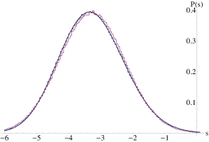
Figure 2: Rescaled PDF of (minus) the free energy at large time. (i) solid line: analytical prediction $\frac{d}{d{\sf s}}F_{4}({\sf s})$. Histograms: (ii) in blue, ground state energy PDF ($T=0$) for a polymer $\hat{t}=2^{10}$ with $N=10^{6}$ samples (iii) in red, PDF of ${\sf s}=-2^{-2/3}f$ for a polymer $\hat{t}=2^{10}$ at $\lambda=6.3$, with $N=10^{6}$ samples. The numerical PDFs are rescaled to adjust the mean and the variance of $F_{4}$. The variable $s$ in all figures is called ${\sf s}$ in the text.

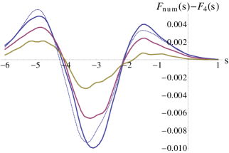
Figure 3: Convergence as a function of $\lambda$: the difference between the numerical CDFs, $F_{num}(s)$, and the prediction for infinite $\lambda$, $F_{4}(s)$, is plotted for $\lambda=0.2\text{ (in blue)},1\text{ (in red)},3\text{ (in yellow)}$ with $N=2.10^{5}$ samples. $\hat{t}=2^{11}$ is hold fixed. For $\lambda=0.2$ a length $\hat{t}=2^{9}$ is also shown (dashed line) illustrating finite size effects. The statistical fluctuations due to finite sample $N$ are visible on the figure.

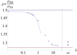
Figure 4: Ratio of variances $\rho=\frac{\sigma_{HS}}{\sigma_{FS}}$, for $\lambda$ varying from $0.2$ to $20$. The crosses correspond to numerical data ($N=2\cdot 10^{5}$ samples, $\hat{t}=2^{11}$, standard error estimation $\epsilon=3\cdot 10^{-3}$). The dashed horizontal lines represent analytic predictions in both limits, $\frac{3}{2}$ for $\lambda\rightarrow 0$ and $\frac{\sigma^{F_{4}}}{\sigma^{F_{2}}}=1.2733$ for $\lambda\rightarrow\infty$. The effect of finite $\hat{t}$ is clearly visible. It causes a small gap between these limits and the numerical data, which decreases as $\hat{t}$ increases. The solid line represents the Taylor expansion (17) globally rescaled to account for finite $\hat{t}$. The right part of the graph shows the convergence of $\rho$ at $T=0$ as a function of $\hat{t}$: the upper point is $\hat{t}=2^{8}$, the lowest $\hat{t}=2^{10}$.

KPZ equation: Let us now detail how our results translate in terms of the KPZ equation

$$\partial_{t}h=\nu\nabla^{2}h+\frac{\lambda_{0}}{2}(\nabla h)^{2}+\eta(x,t)$$ (44)

where $\overline{\eta(x,t)\eta(x^{\prime},t^{\prime})}=R_{\eta}(x-x^{\prime})\delta(t-t^{\prime})$, with Gaussian noise correlator $R_{\eta}(x)=D\delta(x)$. The Cole-Hopf mapping generally implies:

$$\frac{\lambda_{0}}{2\nu}h=\ln Z\quad,\quad\bar{c}=D\lambda_{0}^{2}$$ (45)

Here however we must be more specific. The initial condition (1) corresponds to a wedge $h(x,0)=-w|x-y|$ in the limit $w\to\infty$, before $y\to 0$. Because of the hard wall we have that $\frac{\lambda_{0}}{2\nu}h(x,t)=\ln(xy)+\frac{\lambda_{0}}{2\nu}\tilde{h}(x,t)$ where $\tilde{h}$ is not singular when both $x$ and $y$ approach zero, and the correspondence is really $\frac{\lambda_{0}}{2\nu}\tilde{h}(0,t)=\ln Z$. Schematically the boundary conditions (BC) can be stated as $h(0,t)=-\infty$ or $\nabla h(0,t)=+\infty$ (see more general ones below). Hence from (37):

$$\frac{\lambda_{0}}{2\nu}\tilde{h}(0,t)=\ln\overline{Z}+2^{2/3}\lambda~{}\xi_{t}$$ (46)

with, at large $t$, $\ln\overline{Z}\simeq v_{\infty}t$. From [37, 38], $v_{\infty}=\frac{\lambda_{0}^{2}R_{\eta}(0)}{8\nu^{2}}-\frac{D^{2}\lambda_{0}^{4}}{12}$ is the same non universal constant (see discussion in [42]) in both HS and FS cases, the difference in $\ln\overline{Z}$ being only sublinear in time, as $\sim\ln t$.

Finally, we discuss the universality of our results. The BC we used here at $x=0$ is the hard wall $Z=0$, which in the KPZ context corresponds to $\nabla h=+\infty$. Another standard BC is the reflecting wall (RW) $\nabla Z=0$, i.e. $\nabla h=0$ (contact angle $\pi/2$). For the DP it can be achieved by considering two symmetric half-spaces i.e. $V(-x,t)=V(x,t)$ [44]. At $T=0$ there is no difference in the optimal path energy between the hard and reflecting wall, see Fig. 1. At $T>0$ the two cases become different, since there is more entropy in the RW. However the longer the polymer, the closer it becomes, effectively, to the zero temperature limit. Hence we expect that although at finite time the two cases lead to different $g(s)$, these become equal at large time. In fact all BC such that $\nabla h\geq 0$ should converge to $F_{4}$. This is consistent with the results of [28] translated into the $T=0$ lattice DP model (although the equivalent of the hard wall was not explicitly considered there). In the PNG model it corresponds to the absence of boundary source, or a weak enough source [27]. We will not discuss here the case of BC $\nabla h<0$ which leads to an unbinding transition. A similar transition was studied in the random permutation model [28] and in the PNG model [11, 27], but not using the BA (see however [43]). Work on that case is in progress.

It is worth pointing out an application of our results to the conductance $g$ of disordered 2D conductors deep in the localized regime. Extending the results of Ref. [45] we predict that $L^{-1/3}\ln g$ should be distributed as $F_{4}$ if the leads are small, separated by $L$, and placed near the frontier of the sample (which occupy, say, a half space).

We thank P. Calabrese for numerous discussions and pointing out Ref. [32]. We thank A. Rosso for helpful remarks. We are grateful to N. Crampe, A. Dobrinevski and M. Kardar for interesting discussions and pointing out Ref. [43]. This work was supported by ANR grant 09-BLAN-0097-01/2.

References

• [1] M. Kardar, G. Parisi and Y.C. Zhang, Phys. Rev. Lett. 56, 889 (1986).
• [2] A.-L. Barabasi, H.E. Stanley, Fractal concepts in surface growth, Cambridge University Press (1995); J. Krug, Adv. Phys. 46, 139 (1997).
• [3] M. Kardar and Y-C. Zhang, Phys. Rev. Lett. 58, 2087 (1987); T. Halpin-Healy and Y-C. Zhang, Phys. Rep. 254, 215 (1995).
• [4] K. A. Takeuchi and M. Sano, Phys. Rev. Lett. 104, 230601 (2010); K. A. Takeuchi, M. Sano, T. Sasamoto, and H. Spohn, Sci. Rep. (Nature) 1, 34 (2011).
• [5] L. Miettinen, M. Myllys, J. Merikosks and J. Timonen, Eur. Phys. J. B 46, 55 (2005).
• [6] T. Hwa and M. Lassig, Phys. Rev. Lett. 76, 2591 (1996).
• [7] G. Blatter et al., Rev. Mod. Phys. 66, 1125 (1994). P. Le Doussal, Int. Journal of Modern Physics B, 24 20-21, 3855 (2010).
• [8] S. Lemerle et al., Phys. Rev. Lett. 80, 849 (1998).
• [9] D. A. Huse, C. L. Henley, and D. S. Fisher, Phys. Rev. Lett. 55, 2924 (1985).
• [10] K. Johansson, Comm. Math. Phys. 209, 437 (2000) and arXiv:math/9910146.
• [11] M. Prahofer and H. Spohn, Phys. Rev. Lett. 84, 4882 (2000); J. Stat. Phys. 108, 1071 (2002);
• [12] J. Baik and E.M. Rains, J. Stat. Phys. 100, 523 (2000).
• [13] P. L. Ferrari, Comm. Math. Phys. 252, 77 (2004).
• [14] J. Baik, P. Deift, and K. Johansson, J. Amer. Math. Soc., 12 1119 (1999).
• [15] C. A. Tracy and H. Widom, Comm. Math. Phys. 159, 151 (1994) and 161, 289 (1994).
• [16] I. Corwin, arXiv:1106.1596.
• [17] P. L. Ferrari and H. Spohn, arXiv:1003.0881.
• [18] T. Sasamoto and H. Spohn, Phys. Rev. Lett. 104, 230602 (2010); Nucl. Phys. B 834, 523 (2010); J. Stat. Phys. 140, 209 (2010).
• [19] P. Calabrese, P. Le Doussal and A. Rosso, EPL 90, 20002 (2010).
• [20] V. Dotsenko, EPL 90, 20003 (2010); J. Stat. Mech. P07010 (2010); V. Dotsenko and B. Klumov, J. Stat. Mech. (2010) P03022.
• [21] G. Amir, I. Corwin, J. Quastel, Comm. Pure Appl. Math 64, 466 (2011).
• [22] P. Calabrese and P. Le Doussal, Phys. Rev. Lett. 106, 250603 (2011).
• [23] P. Le Doussal and P. Calabrese, J. Stat. Mech. P06001 (2012).
• [24] T. Imamura, T. Sasamoto, Phys. Rev. Lett. 108, 190603 (2012); J. Phys. A 44, 385001 (2011).
• [25] M. Krech, The Casimir Effect in Critical Systems, (World Scientic, Singapore, 1994); T. Emig, Int. J. Mod. Phys. A 25 2177 (2010).
• [26] P. Le Doussal, K. J. Wiese, EPL 86 22001 (2009).
• [27] T. Sasamoto, T. Imamura, arXiv:cond-mat/0307011, J. Stat. Phys. 115 749 (2004).
• [28] Jinho Baik, Eric M. Rains, arXiv:math/9910019.
• [29] In the large diffusivity, weak noise regime, equivalently high temperature regime for the DP, see below.
• [30] M. Kardar, Nucl. Phys. B 290, 582 (1987).
• [31] E. H. Lieb and W. Liniger, Phys. Rev. 130, 1605 (1963).
• [32] N. Oelkers, M.T. Batchelor, M. Bortz, X.W. Guan, J. Phys. A 39 1073 (2006).
• [33] Y. Hao,Y. Zhang, J. Q. Liang and Shu Chen, Phys. Rev. A 73,063617(2006).
• [34] J. B. McGuire, J. Math. Phys. 5, 622 (1964).
• [35] P. Calabrese and J.-S. Caux, Phys. Rev. Lett. 98, 150403 (2007); J. Stat. Mech. P08032 (2007).
• [36] P. Le Doussal and T. Gueudre, to be published.
• [37] One has $\overline{Z}=1/\sqrt{4\pi t}$ for full space and $\overline{Z}=1/\sqrt{4\pi}t^{3/2}$ with the hard wall, as in absence of disorder. The non-universal global multiplicative constant $e^{R_{V}(0)t/(2T^{2})}$ does not affect the variable $z$ and has been dropped. [42].
• [38] Here we have performed the usual shift $Z=e^{-c^{2}t/12}\hat{Z}$ (we drop the hat below) which does not affect the variable $z=Z/\overline{Z}$.
• [39] J. Baik, R. Buckingham, J. DiFranco, Commun. Math. Phys. 280 463 (2008).
• [40] P.L. Ferrari and H. Spohn, J. Phys. A 38 L557 (2005).
• [41] S. Bustingorry, P. Le Doussal and A. Rosso Phys. Rev. B 82, 140201 (2010).
• [42] T. Gueudre, P. Le Doussal, A. Rosso, A. Henry, P. Calabrese, arXiv:1207.7305
• [43] M. Kardar, Phys. Rev. Lett. 55 2235 (1985).
• [44] Note that if one chooses $V(-x,t)=V(x,t)$ the usual image method works i.e. $Z(x,y,t)\pm Z(x,-y,t)$ is the PS in the half space with reflecting (resp. absorbing) BC.
• [45] A. M. Somoza, M. Ortuno, and J. Prior, Phys. Rev. Letters 99 116602 (2007).